Maintenance Optimization of Offshore Wind Turbines Based on an Opportunistic Maintenance Strategy

Abstract

Owing to the late development of offshore wind power in China, operational data and maintenance experience are relatively scarce. Due to the harsh environmental conditions, a reliability analysis based on limited sample fault data has been regarded as an effective way to investigate maintenance optimization for offshore wind farms. The chief aim of the present work is to develop an effective strategy to reduce the maintenance costs of offshore wind turbines in consideration of their accessibility. The three-parameter Weibull distribution method was applied to failure rate estimation based on limited data. Moreover, considering the impacts of weather conditions on the marine maintenance activities, the Markov method and dynamic time window were used to depict the weather conditions. The opportunistic maintenance strategy was introduced to cut down on the maintenance costs through optimization of the preventive maintenance age and opportunistic maintenance age. The simulation analysis we have performed showed that the maintenance costs of the opportunistic maintenance strategy were 10% lower than those of the preventive maintenance strategy, verifying the effectiveness of the proposed maintenance strategy.

1. Introduction

In recent years, the wind power industry has made rapid progress globally. Due to abundant offshore wind energy resources, the installed capacity and power generation of offshore wind power are growing rapidly [1]. However, considering the large investment and high risk involved in offshore wind power, and the influence of weather conditions, the requirements for offshore wind farms in terms of operation and maintenance vessels, spare-parts management, and other influential factors are more strict. The special operating environment of offshore wind turbines, in which the equipment is affected by natural conditions, such as typhoons, tides, waves, can accelerate the failure of unit components, and the increased failure rate of electrical and mechanical systems finally leads to lower reliability. Thus, the reliability of wind turbines has become an important issue.

The Weibull distribution is an important statistical measure in reliability engineering, known to have good adaptability and availability for various forms of failure rate simulation in relation to mechanical and electrical products. In this paper, the construction of a Weibull equation is pursued. Based on the two-parameter Weibull equation, a location parameter was introduced to create what is known as a three-parameter Weibull equation. Many researchers are interested in three-parameter Weibull equations. In [2], a three-parameter Weibull distribution was used in the asphalt‒concrete fatigue assessment of aging. In [3], optimization of distribution was studied for an inventory system established by Weibull. In [4], a three-parameter Weibull distribution was proposed in a study on the mechanical sector. In [5], the three-parameter Weibull distribution equation was applied to predict wind power density. In [6], a mixed Weibull distribution parameter estimation method was discussed. In [7], the Weibull distribution was studied by using the three best linear unbiased parameter estimation based on previous unbiased estimation and quasi-optimal linearity. This literature review reveals that the three-parameter Weibull equation has been used in many fields, including machinery, architecture, and aerospace; however, so far few applications of the three-parameter Weibull distribution have been used in fault prediction for offshore wind turbines, especially for those with limited fault data.

Moreover, access to offshore wind farms is greatly restricted by wind and wave conditions, which hinders the operation and maintenance of the unit, thus resulting in an increase in outage time, a decrease in the availability of units, and an increase in operation and maintenance costs. It is necessary to consider the impacts of sea weather conditions related to unit operation and maintenance. The impact of weather conditions on wind turbine maintenance strategies has been investigated in previous works. In China, in [8], a wind turbine reliability evaluation method was proposed. Considering the special operating environment of offshore wind turbines, in [9], the impacts of weather, accessibility, and maintenance time on the maintenance strategy of offshore wind turbines were analyzed. In [10], an offshore wind turbine maintenance strategy with minimum cost and maximum reliability was established, considering the influence of wind speed and maintenance waiting time. In [11,12], a normal behavior model was proposed to further investigate wind turbine vibration and fatigue load by using neural networks and a stochastic approach considering the influence of wind speed. In [13], a survey of stochastic models for sea state and different offshore wind farms was made according to the different maintenance schemes of offshore wind turbines, combined with the failure rate and maintenance time for various components of the unit. In [14], a novel method for simulating wind and wave conditions for offshore sites was revealed, and the result indicated that the persistence of weather windows for significant wave height values can be captured by this approach. All these tests show promising results, and the weather model has been deemed accurate enough for simulations of offshore wind parks. Moreover, in [15], a Markov model based on a statistical analysis of wind speed and wave height was established, and finally, the predictions were made for maintenance waiting time. Although there have been some related studies on the effect of weather conditions on offshore wind turbine maintenance strategies, wind speed and wave height have not yet been simultaneously considered to evaluate the accessibility of offshore wind turbine maintenance.

Meanwhile, many researchers have theoretically investigated the opportunistic maintenance strategy from a different perspective. In [16], a two-level maintenance threshold strategy for wind farms was developed, considering opportunistic maintenance and imperfect maintenance based on reliability. In [17], opportunistic condition-based maintenance for systems subjected to degradation and shocks was proposed to determine an optimal maintenance policy for multi-bladed offshore wind turbines. In [18], a new bi-objective opportunistic maintenance optimization model was proposed, and a three-phase discrete event simulation was used to evaluate the performance measures considering the stochastic behavior of wind and limited maintenance capacity. In [19], an opportunistic maintenance approach for wind farms was developed to take advantage of the maintenance opportunities, considering imperfect maintenance actions. In [20], the trade-off between wind farm configuration and the maintenance strategy was investigated by a new bi-objective redundancy and maintenance optimization model.

The primary goal of this research is to carry out studies in an effort to reduce the operating costs of offshore wind turbines. In this paper, the impacts of weather conditions on the maintenance activities are considered, the Markov chain method and dynamic time window are introduced to represent the weather conditions, and a maintenance waiting time is proposed for offshore wind turbines. In addition, the opportunistic maintenance strategy was used to optimize the key components of the maintenance of the offshore wind turbines. Furthermore, the minimum maintenance cost within the maintenance duration was deemed the optimal objective, and the preventive maintenance time and opportunistic maintenance time have been optimized for the main components of wind turbines. In particular, the novelties can be reflected in the following aspects: (1)The three-parameter Weibull method, instead of the two-parameter Weibull method, was applied to the reliability analysis of offshore wind turbines with limited fault data; (2) the Markov chain method was adopted to evaluate the prediction of maintenance waiting time, considering the wind speed and wave height simultaneously; (3) the preventive opportunistic maintenance strategy has proven to be one of the methods available to generate maintenance cost efficiency, instead of the preventive maintenance strategy.

The remainder of this paper is organized as follows. Section 2 introduces the two-parameter Weibull model of onshore wind turbines by the least squares and maximum likelihood methods, and the three-parameter Weibull model of offshore wind turbines by the correlation coefficient, probability-weighted moment, and bilinear regression methods. In Section 3, we describe the construction of a Weibull equation for offshore wind turbines based on scant sample fault data. Section 4 describes the Markov prediction method. In Section 5, we develop an opportunistic maintenance strategy based on accessibility evaluation. Section 6 gives the opportunistic maintenance simulation based on maintenance waiting time. In Section 7, we propose conclusions and recommendations from our study and suggest areas for further research.

2. Reliability Analysis Model for Wind Turbines

For wind turbines, the commonly used reliability analysis model is the Weibull distribution. This distribution is derived from the analysis of material strength by Weibull. It is a very important distribution form in reliability engineering [21]. The probability density function of the Weibull model obtained from the weakest link theory is

$$f\left(t\right)=\{\begin{array}{cc}\frac{\beta }{\alpha }{\left(\frac{t-\gamma }{\alpha }\right)}^{\beta -1}\exp \left[-{\left(\frac{t-\gamma }{\alpha }\right)}^{\beta }\right]& (t\ge \gamma )\\ 0& (t<\gamma )\end{array}$$

(1)

Its distribution function is given by

$$F\left(t\right)=\{\begin{array}{cc}{\displaystyle {\int }_0^{t}f(t)\mathrm{d}t}=1-\exp \left[-{\left(\frac{t-\gamma }{\alpha }\right)}^{\beta }\right]& (t\ge \gamma )\\ 0& (t<\gamma )\end{array}$$

(2)

Its inefficiency function is given by

$$\lambda (t)=\frac{f(t)}{1-F(t)}$$

(3)

In Equations (1) and (2), α is the scale parameter, $\beta$ is the shape parameter, $\beta >0$, and $\gamma$ is the position parameter, $\gamma >0$. $\gamma$ is the threshold value for failure, $\beta$ is used to describe the dispersion of the measured values, and $\alpha$ is related to the average measured values.

In the failure analysis of the product, $\beta$ is associated with the failure mechanism of the product, and the different values of $\beta$ are accompanied by different fault mechanisms. When $\beta <1$, the failure-rate function is a decreasing function, showing the life distribution of products under the wear-out failure period. When $\beta =1$, the failure-rate function is constant, representing the products in the life distribution of the random failure period. When $\beta >1$, the failure-rate function is an increasing function, showing the distribution of products in the period of life [22].

2.1. Weibull Model of Onshore Wind Turbines

For onshore wind turbines, because of their simple operating conditions and abundant operation and fault data, in practical applications, the common assumption is that the device fails at time $\gamma =0$, and the corresponding expressions, Equations (1) and (2), respectively, can be simplified as follows:

$$\begin{array}{cc}f(t)=\frac{\beta }{\alpha }{\left(\frac{t}{\alpha }\right)}^{\beta -1}\exp \left[-{\left(\frac{t}{\alpha }\right)}^{\beta }\right]& (t\ge 0)\end{array},$$

(4)

$$\begin{array}{cc}F(t)=1-\exp \left[-{\left(\frac{t}{\alpha }\right)}^{\beta }\right]& (t\ge 0)\end{array}.$$

(5)

At present, the two-parameter Weibull analysis method is roughly divided into several categories, i.e., least-squares estimation, median rank regression, maximum-likelihood estimation, and method of moments. For engineering purposes, maximum likelihood is usually considered first due to its high accuracy, as compared to method of moment, which tends to be adopted only if the maximum likelihood function will be difficult to construct. In this paper, we used maximum likelihood rather than method of moment.

Practically, median-rank regression can perform well in the case of extreme values occurring when the number of failures is small. Generally, based on the least squares method, the mean variable will be replaced by the median-rank variable so as to alleviate the estimated deviation caused by the extreme value. In this study, the maintenance optimization was based on a small sample, and the extreme value was carved out; therefore, the least squares method, rather than median-rank regression, was pursued, as follows.

2.1.1. Least-Squares Estimation

By the principle of extremum, the equation can be defined as follows:

$$\{\begin{array}{l}\frac{\partial F}{\partial a}=-2{\displaystyle {\displaystyle \sum }_{i=0}^n}{x}_i\left(y_i-a{x}_i-b\right)=0\hfill \\ \frac{\partial F}{\partial b}=-2{\displaystyle {\displaystyle \sum }_{i=0}^n}\left(y_i-a{x}_i-b\right)=0\hfill \end{array}$$

(6)

The solution equation is shown as follows:

$$\{\begin{array}{l}a=\frac{n{\displaystyle {\displaystyle \sum }_{i=0}^n}{x}_i{y}_i-{\displaystyle {\displaystyle \sum }_{i=0}^n}{x}_i{\displaystyle {\displaystyle \sum }_{i=0}^n}{y}_i}{n{\displaystyle \sum _{i=0}^n}{x}_i^2-{\left({\displaystyle {\displaystyle \sum }_{i=0}^n}{x}_i\right)}^2}\hfill \\ b=\frac{1}{n}{\displaystyle {\displaystyle \sum }_{i=1}^n}{y}_i-\frac{a}{n}{\displaystyle {\displaystyle \sum }_{i=1}^n}{x}_i\hfill \end{array}$$

(7)

The two-logarithm transformation of Equation (5) is

$$\ln \left(\ln \left(\frac{1}{1-F(t)}\right)\right)=\beta \ln (t)-\beta \ln (\alpha )$$

(8)

Comparison with the one-element linear-regression equation gives:

$$\{\begin{array}{c}x=\ln (t)\\ y=\ln \left(\ln \left(\frac{1}{1-F(t)}\right)\right)\\ a=\beta \\ b=-\beta \ln \left(\alpha \right)\end{array}$$

(9)

Parameters $\alpha$ and $\beta$ can be obtained from Equation (7).

2.1.2. Maximum-Likelihood Estimation

Maximum-likelihood estimation is an effective method of parameter estimation. It has strong applicability, especially in the case of incomplete life. The basic idea is to select the undetermined parameters first so that the probability of samples appearing in the field of observation is greatest; then the sample value is taken as the unknown parameter’s point estimated value [23].

The likelihood function is

$$L(t_1,t_2,\dots ,t_n,\alpha ,\beta )={\displaystyle \prod _{i=1}^n}\frac{\beta }{\alpha }{\left(\frac{t_i}{\alpha }\right)}^{\beta -1}\exp \left[-{\left(\frac{t_i}{\alpha }\right)}^{\beta }\right]$$

(10)

For the convenience of calculation, the logarithm of Equation (10) is taken as a natural logarithm:

$$\{\begin{array}{c}\ln L\left(t_1,t_2,\dots ,t_n,\alpha ,\beta \right)=n\left(\ln \beta -\ln \alpha \right)+\left(\beta -1\right){{\displaystyle {\displaystyle \sum }_{i=1}^n}\ln \left(\frac{t_i}{\alpha }\right)-{\displaystyle {\displaystyle \sum }_{i=1}^n}\left(\frac{t_i}{\alpha }\right)}^{\beta }\\ \frac{\partial \ln L}{\partial \alpha }=\frac{\partial \ln L}{\partial \beta }=0\end{array}$$

(11)

Then, the likelihood equation is given by

$$\{\begin{array}{l}\frac{\beta }{\alpha }{\displaystyle \sum _{i=1}^n{\left(\frac{t_i}{\alpha }\right)}^{\beta }-\frac{n\beta }{\alpha }=0}\hfill \\ \frac{n}{\beta }+{\displaystyle \sum _{i=1}^n}\ln \left(\frac{t_i}{\alpha }\right)-{\displaystyle \sum _{i=1}^n}\ln {\left(\frac{t_i}{\alpha }\right)}^{\beta }\ln \left(\frac{t_i}{\alpha }\right)=0\hfill \end{array}.$$

(12)

Solving the equation gives the parameters $\alpha$ and $\beta$.

2.2. Weibull Model of Offshore Wind Turbines

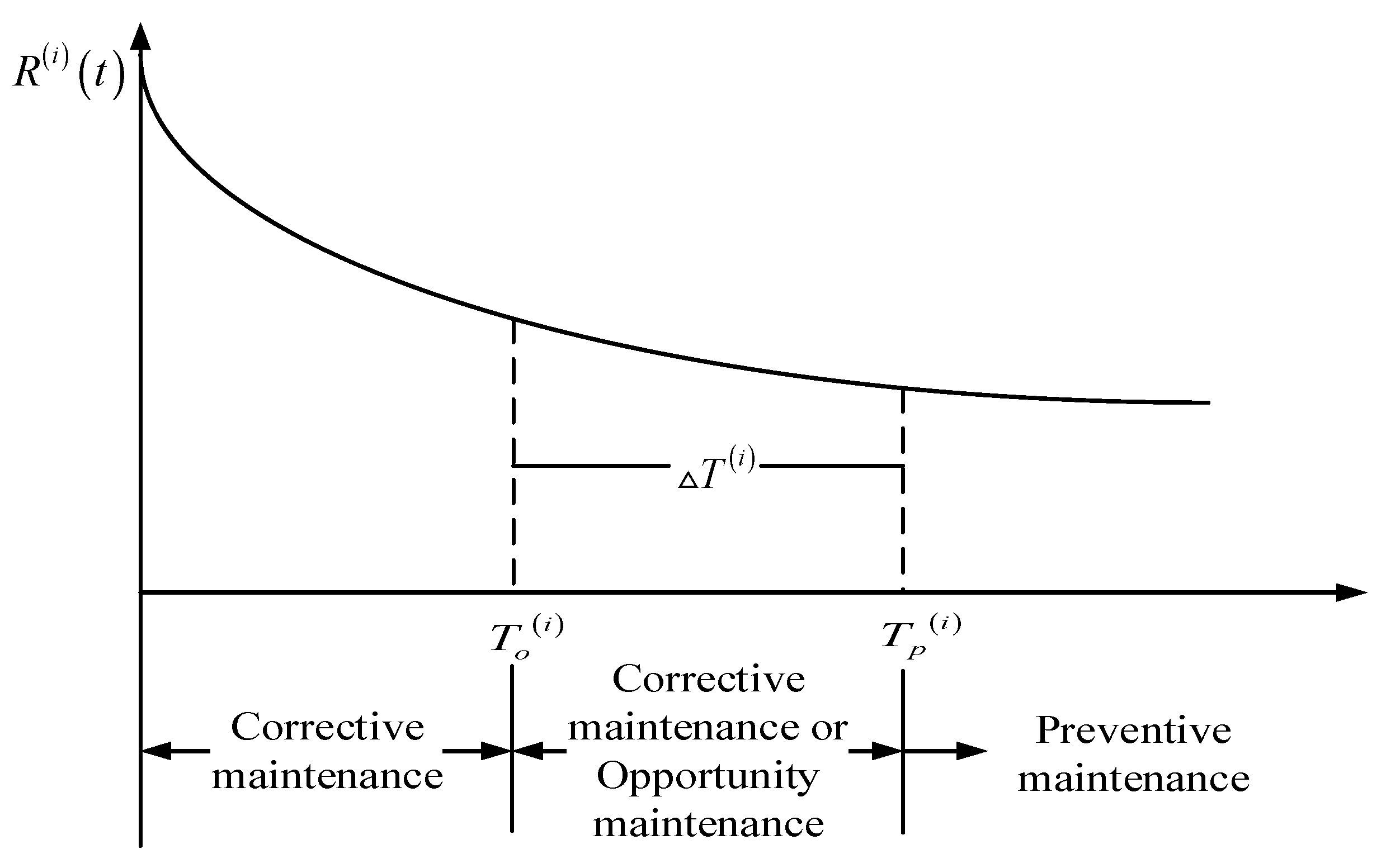
The three-parameter Weibull distribution is used in the life tests of materials with a low stress level, which have better characteristics of curve fitting as compared to the two-parameter Weibull distribution. In the Weibull distribution function, the positional parameter is the threshold value for the failure time of targeted devices and is used to estimate the earliest failure time. Changes in positional parameters will affect the curve displacement of the probability density curve. Generally, when the unit operation time exceeds the positional parameter, the unit starts to fail.

In contrast with onshore wind farms, the conditions of operation and maintenance of offshore wind farms are extremely complicated due to tidewater, typhoons, and corrosion, which result in an increasing probability of the unit components’ failure as well as increased maintenance costs. In addition, due to the particularity of the environment, when a unit failure occurs at an offshore wind farm, maintenance personnel may not be able to reach the site for several months due to harsh weather conditions, which results in difficulty in obtaining component failure data and failure models. Therefore, it is crucial to carry out reliability prediction as soon as possible.

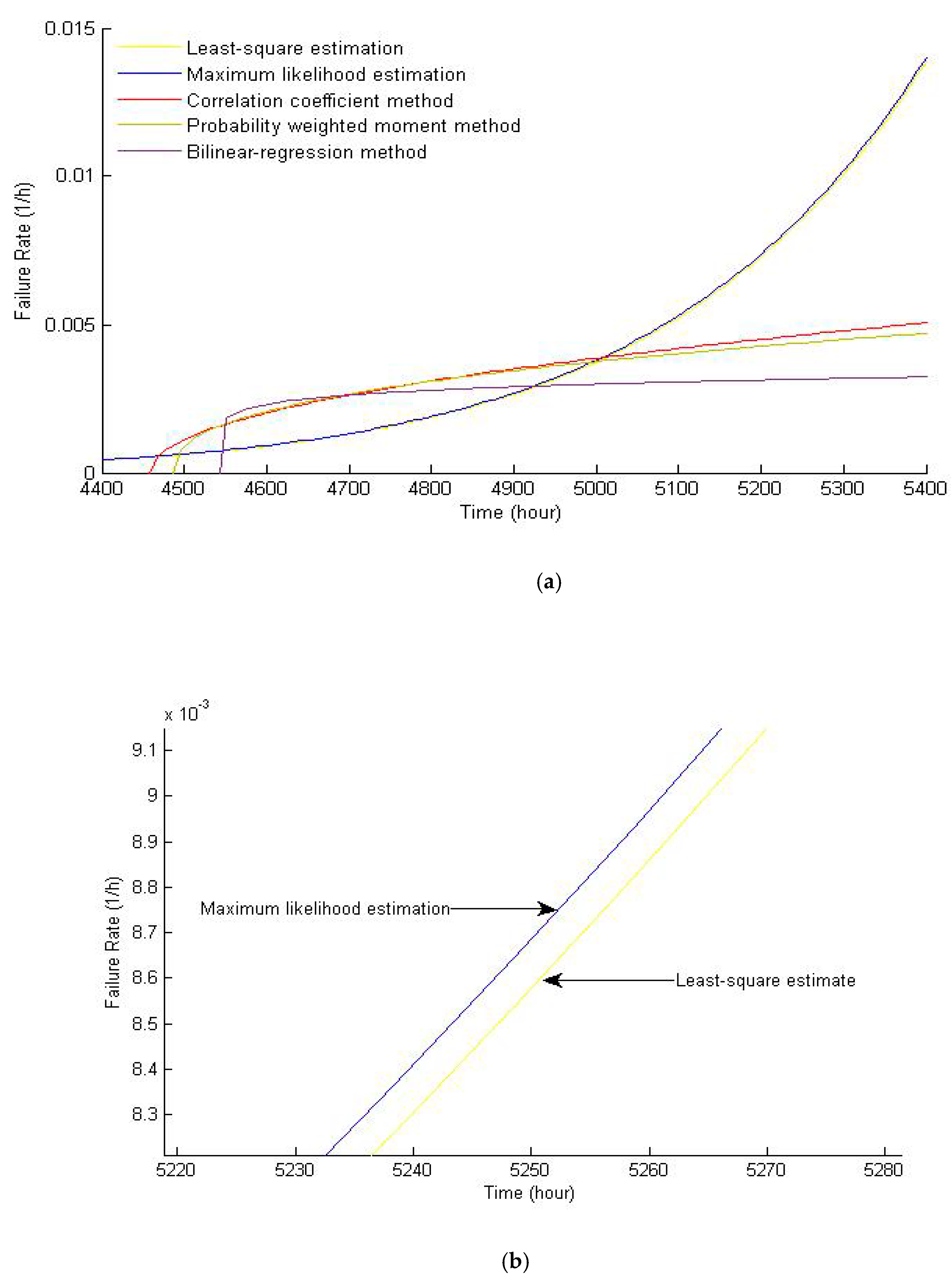
As part of our research, we performed a comparative analysis of the two-parameter Weibull distribution and the three-parameter Weibull distribution. The Weibull three-parameter equation prevails in short-term failure prediction and can be used effectively before t = γ. With regard to short-term failure rate prediction, an abrupt and abnormal rise in the failure rate has taken place under the two-parameter Weibull distribution. On the contrary, the failure rate curve under the three-parameter Weibull distribution displays a rational and smooth rising trend.

However, three parameters exist at the same time, so estimating the parameters of the three-parameter Weibull distribution is difficult. The least-squares method and the maximum-likelihood method are no longer applicable to the three-parameter Weibull distribution. MATLAB is a mathematics software produced by MathWorks. It is a high-level technical computing language and interactive environment for algorithm development, data visualization, data analysis, and numerical calculation, mainly including MATLAB and Simulink. The paper applied MATLAB software for data calculation and simulation.

2.2.1. Correlation Coefficient Method

The two-logarithm transformations of Equation (2) are obtained by

$$\ln \left(\ln \left(\frac{1}{1-F(t)}\right)\right)=\beta \ln (t-\gamma )-\beta \ln (\alpha ).$$

(13)

Equation (13) is changed into

$$\{\begin{array}{c}a=\beta \\ b=-\beta \ln (\alpha )\\ X=\ln (t-\gamma )\\ Y=\beta \ln (t-\gamma )-\beta \ln (\alpha )=aX+b\end{array}$$

(14)

The relationship between X and Y is a linear relationship, as shown in Equation (14). Equation (14) shows that when the estimate of $\gamma$ is correct, a linear relationship exists between X and Y, i.e., the correlation coefficient between X and Y is a maximum. The correlation coefficient $r$ between X and Y is obtained by

$$r=\frac{Cov\left(X,Y\right)}{\sqrt{Var\left[X\right]Var\left[Y\right]}}$$

(15)

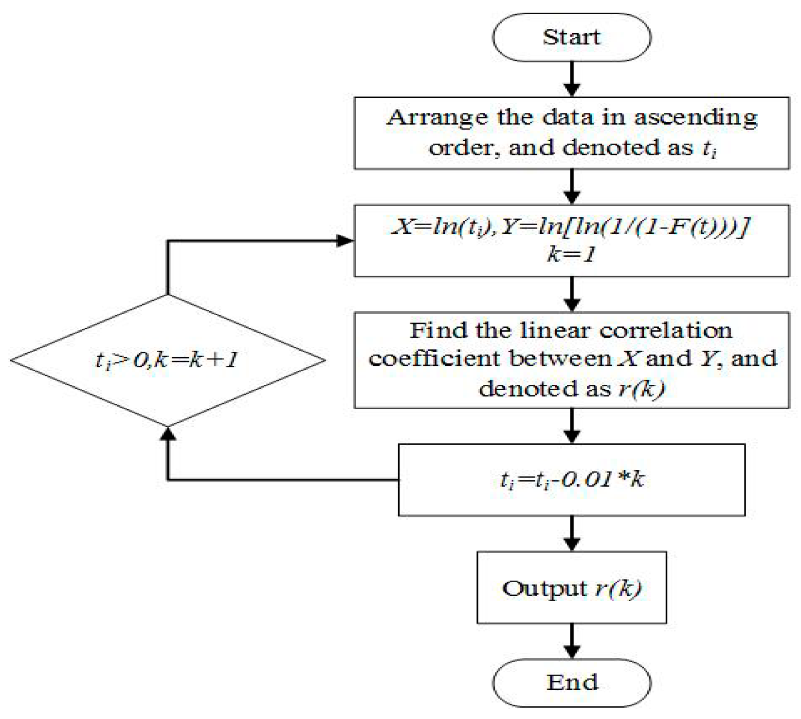
According to the flowchart shown in Figure 1, column vectors containing (k − 1), correlation coefficients are obtained. The step size p can be adjusted according to the actual situation and is selected as 0.01 in the paper. The correlation coefficient $r$ initially increases and then decreases. The position of the corresponding maximum correlation coefficient is found as N, and the optimal estimation value of the position parameter is recorded as

$$\{\begin{array}{c}{t}_i=t_i-(N^2-N)p/2\\ \widehat{\gamma }=(N^2-N)p/2\end{array}$$

(16)

After obtaining the estimated value of the position parameter, we can obtain the estimated value of the parameters by least-squares or maximum-likelihood estimation.

2.2.2. Probability-Weighted Moment Method

For small samples, probability-weighted moments are unbiased and have small errors; this is suitable for the reliability assessment of offshore wind turbines with a small amount of sample data. Therefore, the probability-weighted moments of the sample are used to estimate the distribution parameters, and the accuracy is high.

The inverse probability distribution function for the random variables X of the Weibull three-parameter distribution, which is shown in Equation (17), is obtained using Equations (1) and (2).

$$x=\gamma +\alpha {[-\ln (1-F)]}^{1/\beta }$$

(17)

From this equation, the following can be obtained:

$$M_{1,0,k}=\frac{\gamma }{1+k}+\frac{\alpha \mathsf{\Gamma }(1+1/\beta )}{{(1+k)}^{(1+1/\beta )}}$$

(18)

Let $M_{1,0,k}=M_{(k)}$; then

$$\{\begin{array}{l}{M}_{(0)}=\gamma +\alpha \mathsf{\Gamma }(1+1/\beta )\hfill \\ M_{(1)}=\frac{\gamma }{2}+\frac{\alpha \mathsf{\Gamma }(1+1/\beta )}{2^{(1+1/\beta )}}\hfill \\ M_{(3)}=\frac{\gamma }{4}+\frac{\alpha \mathsf{\Gamma }(1+1/\beta )}{4^{(1+1/\beta )}}\hfill \end{array}$$

(19)

The equation is solved, and the estimated values of parameters $\alpha$, $\beta$, $\gamma$ can be acquired.

$$\{\begin{array}{l}\widehat{\alpha }=\frac{M_{(0)}-\gamma }{\mathsf{\Gamma }\left\{\ln \left[\frac{\left(M_{(0)}-2M_{(1)}\right)}{\left(M_{(1)}-2M_{(3)}\right)}\right]/\ln (2)\right\}}\hfill \\ \widehat{\beta }=\frac{\ln (2)}{\ln \left[\frac{\left(M_{(0)}-2M_{(1)}\right)}{\left(2M_{(1)}-4M_{(3)}\right)}\right]}\hfill \\ \widehat{\gamma }=\frac{4\left[M_{(3)}{M}_{(0)}-M_{(1)}^2\right]}{\left(4M_{(3)}+M_{(0)}-4M_{(1)}\right)}\hfill \end{array}$$

(20)

2.2.3. Bilinear Regression Method

Least-squares estimation is a linear-regression analysis method for a linear equation. It can only be used to solve two-parameter estimation problems. For the estimation of three parameters, two linear equations must be combined.

Let $\alpha =t_0{}^{1/\beta }$; then, Equation (2) can be transformed as follows:

$$\ln \left(\ln \left(\frac{1}{1-F(t)}\right)\right)=\beta \ln (t-\gamma )-\ln (t_0)$$

(21)

$${\left(\ln \left(\frac{1}{1-F(t)}\right)\right)}^{1/\beta }=\frac{t}{\alpha }-\frac{\gamma }{\alpha }$$

(22)

Equations (21) and (22) are linearly independent; they are linear equations that can be expressed as $y_k=a_k{x}_k+b_k,k=1,2$ and $x_i,y_i$ can be depicted, respectively, as

$$\{\begin{array}{ll}{y}_1=\ln \left(\ln \left(\frac{1}{1-F(t)}\right)\right)\hfill & a_1=\beta \hfill \\ x_1=\ln (t-\gamma )\hfill & b_1=-\ln (t_0)\hfill \\ y_2={\left(\ln \left(\frac{1}{1-F(t)}\right)\right)}^{1/\beta }\hfill & a_2=\frac{1}{\alpha }\hfill \\ x_2=t\hfill & b_2=-\frac{\gamma }{\alpha }\hfill \end{array}$$

(23)

According to the least-squares method, Equations (21) and (22) can be substituted into Equation (7) separately, and the combination can be obtained:

$$\{\begin{array}{c}\gamma =\overline{t}-\frac{\left[\overline{t^2}-{(\overline{t})}^2\right]\overline{{\left(\ln \left(\frac{1}{1-F(t)}\right)\right)}^{1/\beta }}}{\overline{t{\left(\ln \left(\frac{1}{1-F(t)}\right)\right)}^{1/\beta }}-\overline{t}\cdot \overline{{\left(\ln \left(\frac{1}{1-F(t)}\right)\right)}^{1/\beta }}}\\ \alpha ={\left[\exp \left(\beta \cdot \overline{\ln (t-\gamma )}-\overline{\ln \left(\ln \left(\frac{1}{1-F(t)}\right)\right)}\right)\right]}^{1/\beta }\\ \beta =\frac{\overline{\ln (t-\gamma )\cdot \ln \left(\ln \left(\frac{1}{1-F(t)}\right)\right)}}{\overline{{(\ln (t-\gamma ))}^2}-{(\overline{\ln (t-\gamma )})}^2}-\frac{\overline{\ln (t-\gamma )}\cdot \overline{\ln \left(\ln \left(\frac{1}{1-F(t)}\right)\right)}}{\overline{{(\ln (t-\gamma ))}^2}-{(\overline{\ln (t-\gamma )})}^2}\end{array}$$

(24)

As long as the accuracy is given, the values of $\beta$ and $\gamma$ can be estimated iteratively, and Equation (24) is substituted to obtain the estimated value of $\alpha$.

3. Analysis of Results

3.1. Verification of Reliability Analysis Method for Wind Turbines

Taking the failure shutdown data of a 3 MW wind turbine at an offshore wind farm in Jiangsu province in China as an example, the method of parameter estimation is verified in this work. The wind farm has 19 wind turbine units installed, each operating at 3 MW, and first operated in June 2017. Typical fault data were collected from the Supervisory Control and Data Acquisition system (SCADA) and selected from July 2017 to July 2018, as shown in

Table 1. Failure times.

Sequence	1	2	3	4	5	6	7	8	9	10	11	12	13
Failure time (h)	4560	4568	4660	4756	4879	4899	4904	4967	4988	4990	4995	4996	4998
Sequence	14	15	16	17	18	19	20	21	22	23	24	25	26
Failure time (h)	4999	5034	5096	5137	5138	5278	5289	5367	5467	5567	5678	5778	5879
Sequence	27	28	29	30	31	32	33	34	35	36	37	38	39
Failure time (h)	5889	5900	6067	6078	6178	6278	6378	6478	6578	6678	6789	6879	6888
Sequence	40	41	42	43	44	45	46	47	48	49	50	51	52
Failure time (h)	6978	6988	6990	7089	7115	7245	7345	7356	7456	7468	7568	7569	7709
Sequence	53	54	55	56
Failure time (h)	7809	7889	7900	7908

.

The method of Weibull parameter estimation proposed in this paper is used to estimate the parameters and failure-rate function of the fault data, as shown in

Table 2. Parameters estimated.

Method	Weibull Distribution Parameters			Failure-Rate Functions
	α	β	γ
Least-squares estimation	4.9979 × 103	18.012	-	4.7388 × 10−66t17.023
Maximum-likelihood estimation	4.9941 × 103	17.963	-	7.2376 × 10−66t16.976
Correlation coefficient method	4.298 × 102	1.487	4462	1.8379 × 10−4 (t − 4457)0.484
Probability-weighted moment	4.069 × 102	1.383	4472	3.2298 × 10−4 (t − 4486)0.393
Bilinear regression method	3.859 × 102	1.144	4513	1.4007 × 10−3 (t − 4543)0.124

. The failure-rate curves of two- and three-parameter Weibull distribution are shown in Figure 2.

According to the failure-rate function estimates given in Table 2, the reliability of the wind turbine is predicted from the last fault time, as shown in

Table 3. Short period prediction on failure rates.

Failure Rate	Two-Parameter		Three-Parameter
	Least-Squares Estimation	Maximum-Likelihood Estimation	Correlation Coefficient Method	Probability-Weighted Moment Method
$\lambda \left(5378\right)$	0.0129	0.0131	0.0050	0.0047
$\lambda \left(8760\right)$	51.7726	51.1463	0.0105	0.0086

.

Comparative analyses are given as follows:

1)

As shown in Table 2, for the two-parameter Weibull distribution, the least-squares, and maximum-likelihood methods are suitable to obtain similar results. For the three-parameter Weibull distribution, the correlation coefficient method, bilinear regression method, and probability-weighted moment method produce similar results.

2)

As shown in Figure 2, given the two-parameter Weibull failure-rate curve from the beginning (t = 0), and the three-parameter Weibull distribution of the failure-rate curve from the beginning (t = γ), the Weibull three-parameter equation prevails for short-term failure prediction of key defects occurring in newly operated wind turbines and can be used to effectively avoid the impact of short-term reliability prediction of atypical failure data before t = γ.

3.2. Simulation Analysis of Maintenance Costs of Wind Turbines

As shown in Figure 3, according to the wind turbine preventive maintenance strategy, the maintenance cost of component i is

$$C_i\left(T_{\mathrm{p}}{}^{\left(i\right)}\right)=\frac{C_{i\mathrm{c}}{F}_i\left(T_{\mathrm{p}}{}^{\left(i\right)}\right)+C_{i\mathrm{p}}\left[1-F_i\left(T_{\mathrm{p}}{}^{\left(i\right)}\right)\right]+C_N}{{\displaystyle {\int }_0^{T_{\mathrm{p}}{}^{\left(i\right)}}tf\left(t\right)\mathrm{d}t+T_{\mathrm{p}}{}^{\left(i\right)}{\displaystyle {\int }_{T_{\mathrm{p}}{}^{\left(i\right)}}^{\infty }f\left(t\right)\mathrm{d}t}}}.$$

(25)

In this equation, $C_{ic}$ is the failure maintenance cost of component $i$; $C_{ip}$ is the preventive maintenance cost of component $i$; $T_p{}^{\left(i\right)}$ is the preventive maintenance service life of component $i$; $C_N$ is the fixed maintenance cost; $C_i\left(T_p{}^{\left(i\right)}\right)$ is the expected cost rate of long-term operation of component $i$ (Chinese ¥/day).

The key components of the wind turbine are subject to Weibull distribution; the distribution parameters are shown in

Table 4. Weibull distribution parameters for major components of wind turbines.

Component	$\mathit{\alpha }$/Day	$\mathit{\beta }$
Blade	3000	2
Gearbox	2400	3
Generator	3300	3

. The maintenance costs are shown in

Table 5. Maintenance costs for the major components of wind turbines.

Component	${\mathit{C}}_{\mathit{i}\mathit{c}}/\yen$	${\mathit{C}}_{\mathit{i}\mathit{p}}/\yen$	${\mathit{C}}_{\mathit{N}}/\yen$
Blade	112,000	28,000	35,000
Gearbox	152,000	38,000
Generator	100,000	25,000

.

Using the two- and three-parameter Weibull reliability analysis methods, the maintenance costs are seen to vary over time, as illustrated in Figure 4, Figure 5 and Figure 6.

Using the two- and three-parameter Weibull reliability analysis methods, the optimal preventive maintenance time and maintenance cost of key components of the wind turbine can be determined; these are shown in

Table 6. Optimal maintenance time and maintenance cost of unit components.

Component	Two-Parameter		Three-Parameter
	${\mathit{T}}_{\mathbf{p}}^{\left(\mathit{i}\right)}/\mathbf{Day}$	$C_i\left(T_{\mathrm{p}}^{\left(i\right)}\right)$	${\mathit{T}}_{\mathbf{p}}^{\left(\mathit{i}\right)}/\mathbf{Day}$	$C_i\left(T_{\mathrm{p}}^{\left(i\right)}\right)$
Blade	2770	51.7344	2490	49.8622
Gearbox	1664	68.4917	1505	63.5657
Generator	2470	38.2659	2284	31.0392

.

It can be seen from Table 6 that the maintenance cost of the unit can be reduced by 8% using the reliability analysis method of the three-parameter Weibull model.

4. Markov Prediction Method

This method uses a mathematical model to analyze the evolution of objects [24]. In the Markov process, the time series is regarded as a stochastic process. By studying the initial probability of different states of things and the state transition matrix, the state change trend is determined, and the future state of things can be predicted. This method has been widely used in communications, biology, the social sciences, and other fields [25].

4.1. Markov Theory

4.1.1. Markov Process

If the random process $\left\{X(t),t\in T\right\}$ satisfies the following condition [26]:

(1)

If the state of the stochastic process $\left\{X(t),t\in T\right\}$ at time t is known, and the state at time t + 1 is only related to the state at time t and independent of the state before time t, then it is considered that the stochastic process $\left\{X(t),t\in T\right\}$ has Markov property.

(2)

When the state space of the stochastic process $\left\{X(t),t\in T\right\}$ is S, if for any n ≥ 2, and any $t_1<t_2<\dots <t_n\in T$ in the condition $X(t_i)=x_i,x_i\in S,i=1,2,\dots ,n-1$, the conditional probability distribution function of $X(t_n)$ is equal to its probability distribution function under the condition $X(t_{n-1})=x_{n-1}$, which is

$$\begin{array}{c}P(X(t_n)\le x_n|X(t_1)=x_1,X(t_2)=x_2,\cdots ,X(t_{n-1})=x_{n-1})\\ =P\left(X(t_n)\le x_n|X(t_{n-1})=x_{n-1}\right)\end{array}$$

(26)

4.1.2. Markov Chain

The Markov chain is a discrete-time stochastic process with Markov property, and the model is usually expressed as $\lambda =(S,P,Q)$, where the meaning of each element is as follows [27]:

1)

S represents a non-empty set of all possible states in a random process. State is the result of a random process occurring at a certain moment. P is a one-step state transition probability matrix. Conditional probability can be expressed as follows:

$$P\left\{X\left(t+1\right)=j|X\left(t\right)=i\right\}=P_{ij}$$

(27)

2)

Q is the initial state probability distribution vector, Let $Q=\left[q_1,q_2,\dots ,q_n\right]$ denote the probability that the stochastic process is in state x_i at time t = 0 is q_i, then

$${\displaystyle \sum _{i=1}^n{q}_i=1}$$

(28)

4.2. Data Processing Based on Markov Method

When using the Markov chain model for predictive analysis, the random variables need to be processed as follows:

(1)

State division of random variables;

(2)

Calculation of state transition probability;

(3)

Test of “Markov property”.

4.2.1. State Division of Random Variables

For the state division of random variables, the following methods are possibilities [28]:

(1)

Sample mean value-mean variance partition method;

(2)

Ordered clustering method;

(3)

Fuzzy clustering method.

In this paper, only the first method is used and will be briefly described below.

Suppose a random observation set of random variable X is $x_1,x_2,\dots ,x_n$, the sample mean is $\overline{x}$, and the sample mean variance is s. If the absolute value $\left|r\right|$ of the auto-correlation coefficients of this set is ≤0.30, it can be approximated as an independent and identically distributed sequence. According to the central limit theorem:

$$\{\begin{array}{l}P\left\{\overline{x}-s\le \overline{x}\le \overline{x}+s\right\}=2\mathsf{\Phi }\left(1.0\right)-1\approx 0.68\\ P\left\{\overline{x}-1.5s\le \overline{x}\le \overline{x}+1.5s\right\}=2\mathsf{\Phi }\left(1.5\right)-1\approx 0.87\end{array}$$

(29)

4.2.2. Calculation of State Transition Probability

Before using the Markov chain for prediction, it is necessary to estimate the transition probability of the Markov chain from the historical observation sequence.

Suppose a set of observation sequences in a random variable X is $x_1,x_2,\dots ,x_m$, which contains n states, namely the state space $S=\left\{1,2,\dots ,n\right\}$. Use f_ij to indicate the frequency of the observation sequence from state i to state j through one step, $i,j\in S$. A matrix ${(f_{ij})}_{i,j\in S}$ composed of $f_{ij}(i,j\in S)$ is called a transfer frequency matrix. The value obtained by dividing the element of the i-th row and the j-th column in the transfer frequency matrix by the sum of the elements of the i-th row is called the maximum likelihood estimation of the transition probability, ${\widehat{P}}_{ij},i,j\in S$, as follows:

$${\widehat{P}}_{ij}=\frac{f_{ij}}{{\displaystyle \sum _{j=1}^n{f}_{ij}}}$$

(30)

4.2.3. Test of “Markov Property”

It is necessary to test whether the random variable sequence has “Markov property” before applying the Markov chain model to solve practical problems. Usually, a discrete sequence of the Markov chain can be tested using the ${\chi }^2$ statistic.

The marginal probability is denoted as $P_{·j}$, as follows:

$$P_{·j}=\frac{{\displaystyle \sum _{i=1}^n{f}_{ij}}}{{\displaystyle \sum _{i=1}^n{\displaystyle \sum _{j=1}^n{f}_{ij}}}}$$

(31)

Then, when n is sufficiently large, the statistics obeys the ${\chi }^2$ distribution with a degree of freedom of ${(n-1)}^2$, where P_ij is the transition probability.

$${\chi }^2=2{\displaystyle \sum _{i=1}^n{\displaystyle \sum _{j=1}^n{f}_{ij}\left|\log \frac{P_{ij}}{P_{·j}}\right|}}$$

(32)

Given the significance level $\alpha$, we can get the value of ${\chi }_{\alpha }^2{(n-1)}^2$ from the lookup table, and finally calculate the value of the available statistic ${\chi }_{\alpha }^2$. If ${\chi }_{\alpha }^2>{\chi }_{\alpha }^2{(n-1)}^2$, it can be considered that the random sequences $x_1,x_2,\dots ,x_m$ have “Markov property” [29].

4.3. Markov Prediction Model

The operation and maintenance of offshore wind turbines are affected by weather conditions, such as sea wind speed and wind direction, and sea conditions, such as wave height and cycle. Among them, wind speed and wave height are the two most important factors affecting the accessibility of wind turbines [30]. As a consequence, in this paper, the accessibility of offshore wind turbines is studied mainly by considering the wind speed and wave height.

Offshore wind speed and wave height are characterized by time variation and randomness. Commonly used research methods include Gaussian statistics, the Markov method, and the auto-regressive moving average method. The Markov method was used to build the model since the method can accurately describe the long-term and seasonal wind speed and wave height distribution [31].

There are three main methods for Markov chain prediction [32]:

(1)

Markov chain prediction based on absolute distribution;

(2)

Superimposed Markov chain prediction;

(3)

Weighted Markov chain prediction.

In the case of unrestricted visual conditions, the operation and maintenance of offshore wind farms only need to consider the effects of wind speed and wave height. On the other hand, according to the monitoring of coastal sea conditions by the National Ocean Forecasting Station, the relationship between the average wind speed at sea and the effective wave height can be expressed as in Equation (33) [33]:

$$H_s=0.038V^{2.0}+0.1950$$

(33)

where H_s is the effective wave height, and V represents the wind speed. Based on this, the paper simplifies the weather conditions at sea, and the wind speed prediction value can be obtained according to Equation (33).

Due to the fact that the wind speed and wave height at sea have obvious periodicity and seasonality and the state transition probability satisfies the “time homogeneity” characteristic, this paper uses the Markov chain prediction method based on absolute distribution to model the weather of offshore wind farms. The detailed method and steps for modeling are as follows:

(1)

State division of historical observation data of wind speed and wave height. In this paper, ∆H_s = 0.1 m, ∆V = 1 m/s or ∆H_s = 0.4 m, ∆V = 1 m/s were used as the standard interval grouping method to classify the state of the sea wind and waves.

(2)

According to the state group established by step (1), a frequency transfer matrix ${(f_{ij})}_{i,j\in S}$ and a Markov chain state transition probability matrix ${({\widehat{P}}_{ij})}_{i,j\in S}$ having a step size of one can be obtained.

(3)

Test of “Markov property”.

(4)

If the state at time t is known at which the wind speed and the wave height is i, the initial distribution can be considered to be as follows:

$$P\left(0\right)=\left(0,\cdots ,0,1,0,\cdots ,0\right)$$

(34)

The absolute distribution of wind speed and wave height at t + 1 is

$$P\left(1\right)=P\left(0\right)P=\left(p_{i1},p_{i2},\cdots ,p_{in}\right)$$

(35)

The predicted state j at time t + 1 satisfies Equation (36):

$$p_{ij}=\max \left\{p_{ij},j\in S\right\}S=\left\{1,2,\cdots ,n\right\}$$

(36)

Then, the wind speed and wave height at time t + k can be obtained.

(5)

Duration prediction of accessibility and inaccessible state. According to the current ship performance and sea level in China, referring to the domestic and foreign related literature [34], and combined with the weather and ocean conditions in the sea area where the offshore wind farm is located, the operation and maintenance of offshore wind farms are generally operated at wind speed V ≤ 10 m/s and wave height H_s ≤ 2 m. According to Equation (32), when the wave height is less than 2 m, the wind speed can meet the ship’s sea conditions. Therefore, the paper only needs to consider the wave height.

Suppose H is a set of accessibility states that contains multiple wind speeds and wave height states; according to Equation (36), the one-step state transition probability matrix $\tilde{P}$ for H and its complement $S-H$ (denoted as $\tilde{H}$) can be obtained. The steady-state distribution vector is $\tilde{\pi }=\left\{{\tilde{\pi }}_H,{\tilde{\pi }}_{\tilde{H}}\right\}$, where ${\tilde{\pi }}_H,{\tilde{\pi }}_{\tilde{H}}$ represent the probability of state set H and $\tilde{H}$, respectively.

$$\tilde{P}=\left[\begin{array}{cc}{\tilde{p}}_{HH}& {\tilde{p}}_{H\tilde{H}}\\ {\tilde{p}}_{\tilde{H}H}& {\tilde{p}}_{\tilde{H}\tilde{H}}\end{array}\right]$$

(37)

Assuming that $\tau (\tau =1,2,\dots ,l)$ is the duration of the state set H, the probability that the state set H lasts for l durations is

$$\begin{array}{l}p\left\{\tau =l\right\}=p\left\{X_1\in H,X_2\in H,\cdots ,X_l\in H|X_0\in \tilde{H},X_{l+1}\in \tilde{H}\right\}\\ ={\tilde{\pi }}_2{\tilde{p}}_{21}{\left({\tilde{p}}_{11}\right)}^{l-1}{\tilde{p}}_{12}\end{array}$$

(38)

where $X_1,X_2,X_s,X_l$ represent the states of the first, second, s-th, and l-th periods, respectively. Then, the average duration E(τ) can be obtained according to Equation (39):

$$E\left(\tau \right)={\displaystyle \sum _{i=1}^{\infty }p\left\{\tau =i\right\}i}$$

(39)

Similarly, the probability $\tilde{p}\left\{\tau =l\right\}$ of the state $\tilde{H}$ lasting for l periods of time and the average duration $\tilde{E}(\tau )$ are

$$\tilde{p}\left\{\tau =l\right\}={\tilde{\pi }}_1{\tilde{p}}_{12}{\left({\tilde{p}}_{22}\right)}^{l-1}{\tilde{p}}_{21}$$

(40)

$$\tilde{E}\left(\tau \right)={\displaystyle \sum _{i=1}^{\infty }\tilde{p}\left\{\tau =i\right\}i}$$

(41)

(6)

Maintenance waiting time prediction analysis. The operation and maintenance of offshore wind turbines are affected by climate and tides, resulting in increased waiting time for maintenance and limited actual maintenance time. Assuming that personnel, vessels, spare parts, etc., are adequately prepared, the waiting time for maintenance depends only on the weather conditions.

Assuming that the unit components fail at time $t$ and the total time required for failure repair and transportation is $t_n$, the maintenance waiting time can be estimated using the dynamic time window. The specific steps are as follows:

1)

Determine the season $w$ at time $t$, and then calculate the cumulative probability distribution based on the probability (${\pi }_w$) of each state in the season. A random number between (0, 1) is generated, and the cumulative probability distribution interval in which the random number is located is determined; thereby, a state $X_{t,w}$ of the wind speed and the wave height at the same moment can be obtained.

2)

If $X_{t,w}\in H$, then initialize the duration $t_{lo}=\Delta t$ of the reachable state and the maintenance waiting time $t_{wa}=0$; if not, let $t_{lo}=0$, $t_{wa}=\Delta t$, where ∆t is the Markov model step size.

3)

According to the one-step state transition matrix $P_w$, the probability vector of the state $X_{t,w}$ converted to the next moment state is $P_{X,w}$, and $X_{t,w}=P_{X,w}$. The next time state $X_{t+1,w}$ is obtained according to the method in step (1).

4)

If $X_{t+1,w}\in H$, update the reachable state duration $t_{lo}=t_{lo}+\Delta t$, $t=t+1$; otherwise, $t_{lo}=0$, $t_{wa}=t_{lo}+\Delta t$, $t=t+1$.

5)

Repeat steps (3) and (4) until $t_{lo}\ge t_n$, where $t_{wa}$ is the waiting time for this maintenance activity.

5. An Opportunistic Maintenance Strategy Based on Accessibility Evaluation

A wind turbine is a complex multi-component system. Once a component fails, the functions of other components will also be affected, resulting in overall shutdown and the need for maintenance of the unit. The paper intends to study a maintenance strategy for offshore wind turbines in combination with equipment fault repair and preventive maintenance.

5.1. Opportunistic Maintenance Strategy

The opportunistic maintenance strategy refers to the fact that, when a component in the system is repaired or replaced due to a malfunction or other reason, it also provides an opportunity for preventive maintenance or replacement of other components, considering the fact that the maintenance of multiple parts at the same time can effectively save fixed maintenance costs and increase availability.

The principle of the opportunistic maintenance strategy for failure repair combined with preventive maintenance of components is shown in Figure 7.

5.2. Opportunistic Maintenance Model

5.2.1. Opportunistic Maintenance Probability Density Function

According to the opportunistic maintenance strategy in Figure 7, the expected replacement rate of the component consists of three parts, complete replacement, incomplete repair, and minimum maintenance. This paper only considers the opportunistic maintenance strategy for a complete replacement. According to the update process theory, when the component is repaired for a period of time, the maintenance rate is close to constant, which is the reciprocal of the expected replacement cycle of the component. According to the opportunistic maintenance strategy shown in Figure 7, the replacement rate ${\lambda }_i$ of one component consists of three parts, as shown in Equation (42):

$${\lambda }_i=1/E_i\left(T\right)={\lambda }_{ci}+{\lambda }_{oi}+{\lambda }_{pi}$$

(42)

where ${\lambda }_i=P_i(f)\times {\lambda }_i$; ${\lambda }_{oi}=P_i(o)\times {\lambda }_i$; ${\lambda }_{pi}=P_i(p)\times {\lambda }_i$ are the failure replacement rate, opportunistic replacement rate, and preventive replacement rate of one component, respectively. $P_i$ is the replacement probability and $E_i(T)$ is the expected life of the component.

Since the opportunistic replacement of component i is caused by the failure replacement or preventive replacement of other components, the opportunistic replacement probability density function of the component i can be approximated as an exponential distribution function, as follows:

$$g_i\left(t,T_o{}^{\left(i\right)}\right)={\delta }_i\exp \left[-{\delta }_i(t-T_o{}^{\left(i\right)})\right]$$

(43)

$${\delta }_i={\displaystyle \sum _{j\ne i}^N\left({\lambda }_{ci}+{\lambda }_{pi}\right)}$$

(44)

where $g_i(t,T_o^{(i)})$ represents the opportunistic replacement probability density function of the component $i$, ${\delta }_i$ is the exponential distribution function, and N is the number of key components of the unit.

5.2.2. Key Component Replacement Probability of the Wind Turbine

According to the opportunistic maintenance strategy shown in Figure 7, the probability of each replacement is as follows:

$$P_i\left(c\right)={\displaystyle {\int }_0^{T_o{}^{\left(i\right)}}{f}_i\left(t\right)dt+{\displaystyle {\int }_{T_o{}^{\left(i\right)}}^{T_p{}^{\left(i\right)}}{f}_i\left(t\right)\times {\overline{G}}_i\left(t,T_o{}^{\left(i\right)}\right)}}dt,$$

(45)

$$P_i\left(o\right)={\displaystyle {\int }_{T_o{}^{\left(i\right)}}^{T_p{}^{\left(i\right)}}{\overline{F}}_i\left(t\right)\times {\overline{g}}_i\left(t,T_o{}^{\left(i\right)}\right)}dt,$$

(46)

$$P_i\left(p\right)={\overline{F}}_i\left(T_p{}^{\left(i\right)}\right)\times {\overline{G}}_i\left(T_p{}^{\left(i\right)},T_o{}^{\left(i\right)}\right),$$

(47)

$${\overline{F}}_i\left(t\right)=1-{\displaystyle {\int }_0^t{f}_i\left(u\right)du},$$

(48)

$${\overline{G}}_i\left(t,T_o{}^{\left(i\right)}\right)=1-{\displaystyle {\int }_{T_{oi}}^t{g}_i\left(u,T_o{}^{\left(i\right)}\right)}du,$$

(49)

where $f_i(t)$ is the failure probability density function of component i, which obeys the Weibull distribution.

5.2.3. Opportunistic Maintenance Optimization Model

During one replacement cycle of a wind turbine component, the maintenance cost of component i consists of replacement costs, downtime losses, and rental vessel costs. The expected repair cost of component i during a replacement cycle can be expressed as follows:

$$\begin{array}{ll}{E}_i\left(C\right)& =\left[C_{ci}+(t_{wa}+t_n)C_e\right]P_i\left(c\right)+C_{oi}{P}_i\left(o\right)\\ & +\left[C_{pi}+(t_{wa}+t_n)C_e\right]P_i\left(p\right)+C_N\end{array}$$

(50)

where $C_{ci}$, $C_{pi}$, $C_{oi}$ represent the costs of failure maintenance, preventive maintenance, and opportunistic maintenance, respectively, of component i; $C_e$ is the loss per unit downtime, and $C_N$ is the rental vessel cost.

During one replacement cycle of a wind turbine component, the expected life of component i can be expressed as follows:

$$\begin{array}{ll}{E}_i\left(T\right)& ={\displaystyle {\int }_0^{T_o{}^{\left(i\right)}}t\times f_i\left(t\right)}dt+T_p{}^{\left(i\right)}\times \overline{F_i}\left(T_p{}^{\left(i\right)}\right)\times \overline{G_i}\left(T_p{}^{\left(i\right)},T_o{}^{\left(i\right)}\right)\\ & +{\displaystyle {\int }_{T_o{}^{\left(i\right)}}^{T_p{}^{\left(i\right)}}t\left[f_i\left(t\right)\times \overline{G_i}\left(t,T_o{}^{\left(i\right)}\right)+\overline{F_i}\left(t\right)\times g_t\left(t,T_o{}^{\left(i\right)}\right)\right]dt}\end{array}$$

(51)

According to the above analysis, by optimizing the opportunistic maintenance age and preventive maintenance service age of each key component of the unit to minimize the average cost rate, the following optimization model is established:

$$\begin{array}{c}\min Z\left(T_o,T_p\right)={\displaystyle \sum _{i=1}^N\frac{E_i\left(C\right)}{E_i\left(T\right)}}\hfill \\ s.t.0<T_o<T_p\hfill \\ t_{lo}\ge t_n\end{array}$$

(52)

where $Z(T_o,T_p)$ is the average cost rate of the unit.

6. Simulation Analysis

6.1. Accessibility Evaluation Simulation Analysis

Due to a lack of weather and ocean data for offshore wind farms, this paper takes the historical observation data from an observation station in the Yangtze River estuary (30° N, 128° E) in the East China Sea as an example to model the sea weather.

The data on wind speed and wave height in the article were recorded every half hour from 0:00 on 1 January 2014. The 17,306 data points recorded in 2014 were used to make a forecast analysis of wind speed and wave height in 2015.

6.1.1. Wind Speed and Wave Height State Prediction

Using the Markov method, the wind speed and wave height can be divided into n states, and the state set is S = {1,2,⋯,n}. In this paper, $H_s$ = 0.1 m, 0.2 m, 0.3 m, 0.4 m are used as grouping criteria to predict the 100 data points of wind speed and wave height in January 2015. The results are shown in Figure 8, Figure 9, Figure 10 and Figure 11.

The difference between the predicted data and the observed data and the correlation coefficient are used as criteria of the quality of the predicted data. The correlation coefficients of the observed and predicted data of average wind speed and average wave height are calculated separately, as shown in

Table 7. Comparison of observation and prediction data.

$\mathbf{\Delta }{\mathit{H}}_{\mathit{s}}\left(\mathbf{m}\right)$	V(m/s)	${\mathit{H}}_{\mathit{s}}\left(\mathbf{m}\right)$	d(m)	$r$
0	9.9300	4.5618	0	1.0000
0.1	9.2756	3.9360	16.0764	0.8742
0.2	9.7762	4.1960	17.7252	0.8235
0.3	8.1154	3.6840	18.6377	0.8712
0.4	8.7624	3.5240	19.3732	0.8525

.

In Table 7, the data of the wind speed and wave height when $\Delta H_s=0$ are observed data; r is the correlation coefficients of the observed and predicted data; d is the absolute error of prediction data and observation data of the wave height, expressed as in Equation (52):

$$d={\displaystyle \sum _{i=1}^{100}\left|{\left(H_s\right)}_{predictivevalue}-{\left(H_s\right)}_{observedvalue}\right|}$$

(53)

Taking the average error of the wave height prediction data as a standard to measure the advantages and disadvantages of different state grouping methods, the average error, corresponding to $H_s$ = 0.1 m, 0.2 m, 0.3 m, 0.4 m, is shown in Figure 12.

From Figure 12, when $\Delta H_s=0.1$ m, the average error of wave height prediction data and observation data reached the minimum, which means the state grouping method of $\Delta H_s=0.1$ m is superior to the other three groups. As a consequence, this state grouping method is used as a grouping criterion for the state in the following.

6.1.2. Duration Prediction of Wind Speed and Wave Height

Markov models are established for each of the four seasons. The occurrence probability of the accessible state H and the inaccessible state $\tilde{H}$ in different seasons is shown in Figure 13.

The duration of each state under different seasons is shown in

Table 8. The duration of each state under each season.

State	Persistence
	Spring	Summer	Autumn	Winter
H	0.624	0.786	0.570	0.455
$\tilde{H}$	0.376	0.214	0.430	0.545

. One duration is the step size of the Markov model, which is 0.5 h.

Take the inaccessible state $\tilde{H}$ in January 2015 as an example, the observed and predicted values of the probability distribution and the cumulative distribution of the state duration are presented in Figure 14, which shows the accuracy of the Markov chain model.

According to Figure 13 and Table 8, the occurrence probability of accessibility in summer is larger than in any other seasons, and the average duration is the longest, indicating that the wind speed and wave height in summer are more suitable for sea. On the contrary, the occurrence probability of the inaccessible state in winter is the largest, indicating that the wind speed and wave height are not suitable, and the bad weather will last for a long time.

6.1.3. Maintenance Waiting Time Estimate

Taking the maintenance waiting time in January 2015 as an example, the relationship between the maintenance waiting time and the state of the reachable state is shown in Figure 13. One duration is set to be 0.5 h. It can be seen that the waiting time for maintenance increases with the duration of the accessible state.

As seen in Figure 15, at the initial moment, there is a large difference between the predicted value and the observed value when $\Delta H_s=0.1$ m. As the duration increases, the observations gradually approach the predicted value, and finally, only a small gap is observed. When $\Delta H_s=0.4$ m, the predicted value is far from the observed value at the initial moment; as the duration increases, the gap decreases, but in the end, it still maintains a large gap.

6.2. Simulation Analysis of the Opportunistic Maintenance Strategy

In this paper, a 3 MW wind turbine in an offshore wind farm in China is used as an example to optimize the opportunistic maintenance strategy for the critical components of the unit, including the gearbox, the main bearing, and the generator. According to the analysis of the statistical data of failure record of the unit, the failure time of the component follows the Weibull distribution, and the specific parameters are shown in

Table 9. Weibull distribution parameters and maintenance costs of critical components.

Component Number	${\mathit{\alpha }}_{\mathit{i}}/\mathbf{Day}$	${\mathit{\beta }}_{\mathit{i}}$	${\mathit{\gamma }}_{\mathit{i}}/\mathbf{Day}$	$C_{1i}$/Yuan	$C_{2i}$/Yuan
1	2529	2.8	465	672,000	168,000
2	2228	2.5	136	912,000	228,000
3	4036	2.5	91	360,000	90,000
4	3154	2.2	36	600,000	150,000

below, where 1, 2, 3, and 4 represent the blade, gearbox, main bearing, and generator, respectively; α and β are the shape parameters and scale parameters of the components, respectively; unit downtime loss $C_e$ = 720 yuan/h; and the ship chartering fee $C_N$ = 150,000 yuan/day.

When the traditional age-preventive maintenance strategy is adopted, the preventive maintenance age of the critical components of the unit is optimized to minimize the average cost rate. The results after optimization are shown in

Table 10. Optimization results of age maintenance strategy.

Component	Preventive Maintenance Age Tp/Day	Minimum Cost Rate/¥ Day−2	Total Minimum Cost Rate/¥ Day−1
Blade	1816	184.8898	782.6744
Gearbox	1423	300.5747
Main bearing	2822	108.3843
Generator	2284	188.8256

.

When using a multi-component opportunistic maintenance strategy, the opportunistic maintenance age, and preventive maintenance age of the components are optimized to minimize the average cost rate. The results are shown in

Table 11. Optimization results of the opportunistic maintenance strategy.

Component	Opportunistic Maintenance Age To/Day	Preventive Maintenance Age Tp/Day	Total Minimum Cost Rate/¥ Day−1
Blade	721	2709	702.5834
Gearbox	639	1812
Main bearing	1001	3000
Generator	897	2430

.

From the comparison of the results in Table 10 and Table 11, it can be seen that the maintenance cost of the wind turbine using the opportunistic maintenance strategy is 10% lower than that of the preventive maintenance strategy.

Although the proposed model gains competitiveness in terms of the unit maintenance cost, its limitations are as follows:

(1)

The research on the maintenance cost was aimed at the key components of a single wind turbine rather than multiple wind turbines.

(2)

Influential factors, such as the availability of vessels, the adequacy of the spare parts, and the meteorological conditions, were linked to maintenance waiting time. In this paper, wind speed and wave height were considered in the determination of maintenance waiting time, assuming vessels and spare parts were available.

7. Conclusions

Before concluding, one additional point needs to be discussed. Because the operating environment of offshore wind turbines is complex, wind is a crucial factor that should be considered in optimal maintenance decisions. Moreover, the randomness of wind impacts on the power generated by wind turbines, which contributes to unsatisfactory energy costs. In this paper, the influence that fluctuations in wind speed had on the costs of offshore wind farming was considered in the determination of maintenance waiting time. From the perspective of reducing the entire-life costs of an offshore wind farm, we paid attention to how much maintenance costs will be reduced with the introduction of the opportunistic maintenance strategy. Actually, in this sense, how the wind fluctuation will act on the unit cost is not the research priority in this study. Indeed, the influence of wind fluctuation and grid impact on the unit is worth intensively study in further research.

In this paper, we attempted to analyze the characteristics of operation data of offshore wind turbines and investigated reliability analysis methods for offshore wind turbines based on limited fault data. Considering the influence of weather factors, such as wind speed and wave height, we studied maintenance waiting time prediction methods for offshore wind turbines. Combining failure maintenance and preventive maintenance, we proposed an opportunity-based offshore wind turbine maintenance strategy. The main study results are as follows:

(1)

The construction of a Weibull equation for offshore wind turbines was based on a small amount of sample fault data. Different to [8], based on the construction of a two-parameter Weibull equation, a three-parameter Weibull equation was proposed. The results show that the maintenance costs can be reduced by 8% with the adoption of a three-parameter Weibull model, and the fitting curve and failure rate short-term prediction of the three-parameter Weibull distribution is superior to the two-parameter Weibull distribution where there are limited fault data;

(2)

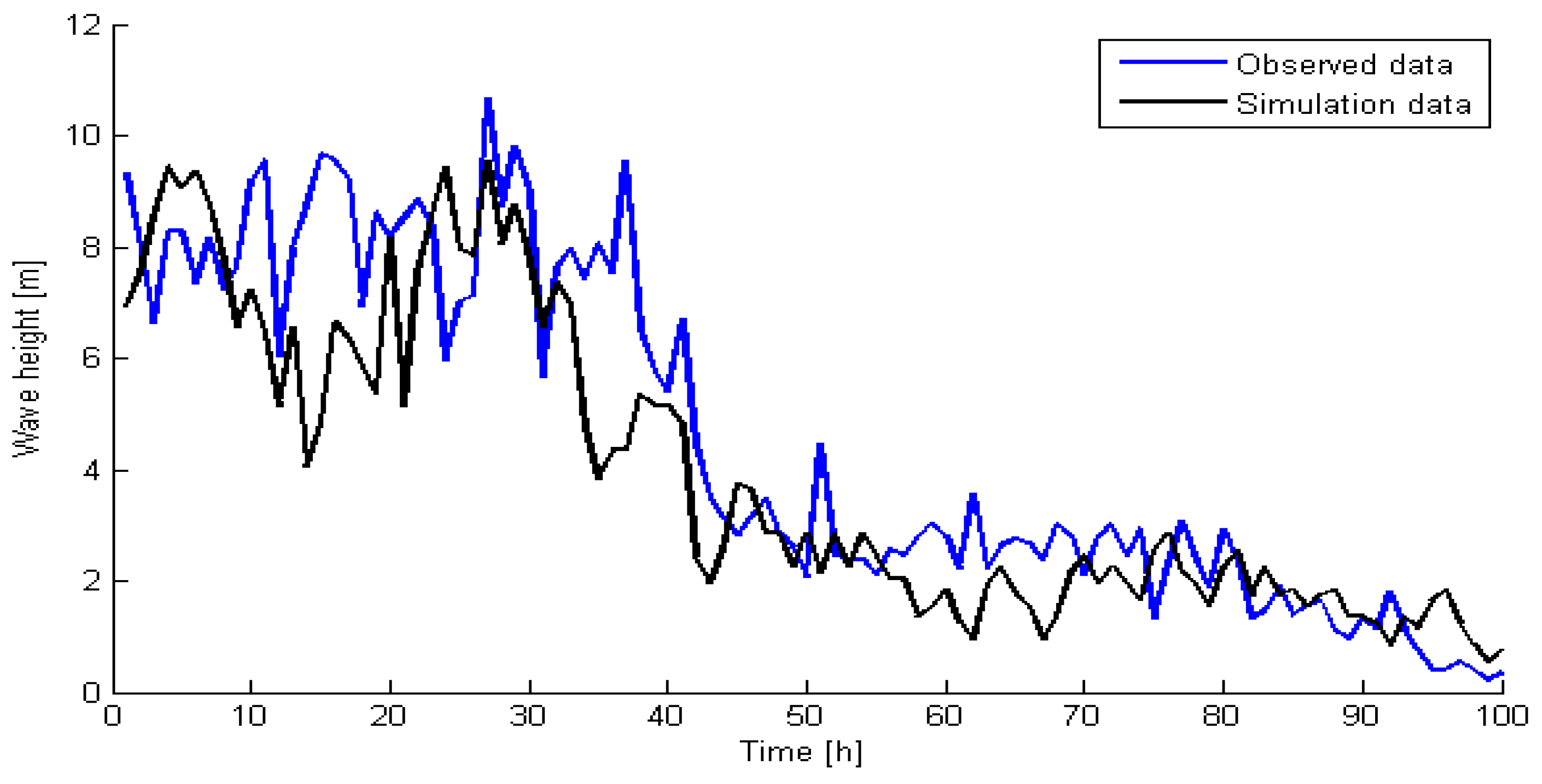
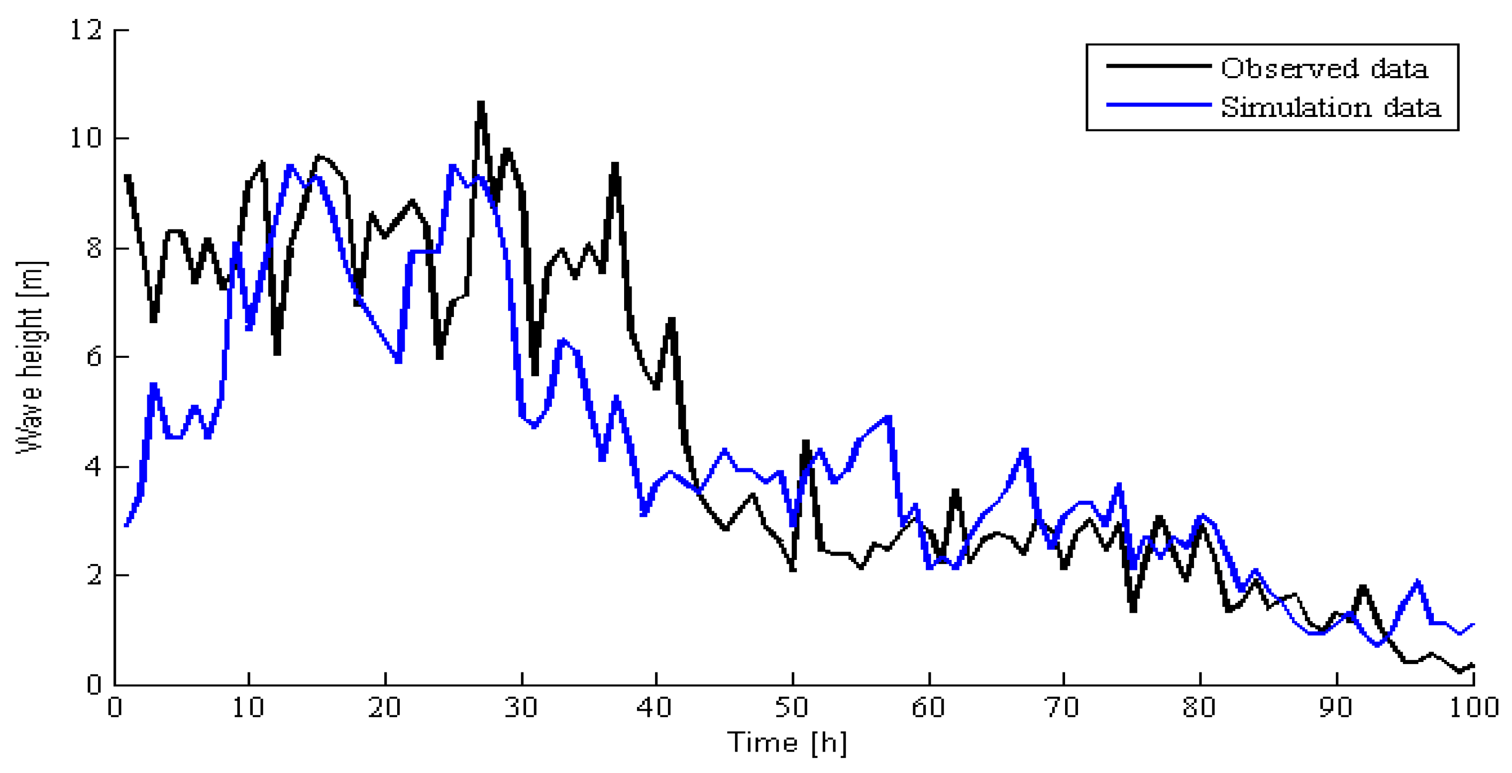
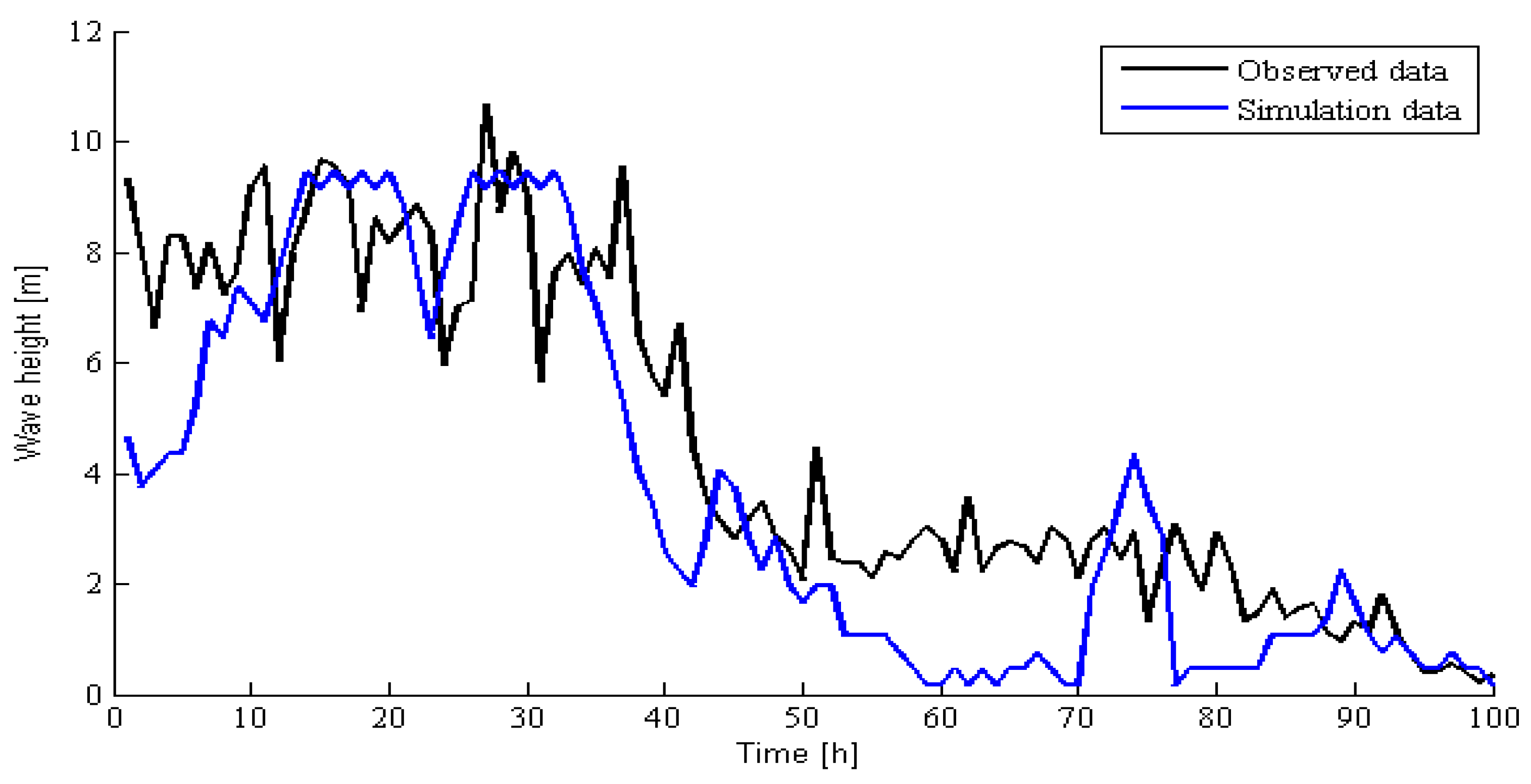
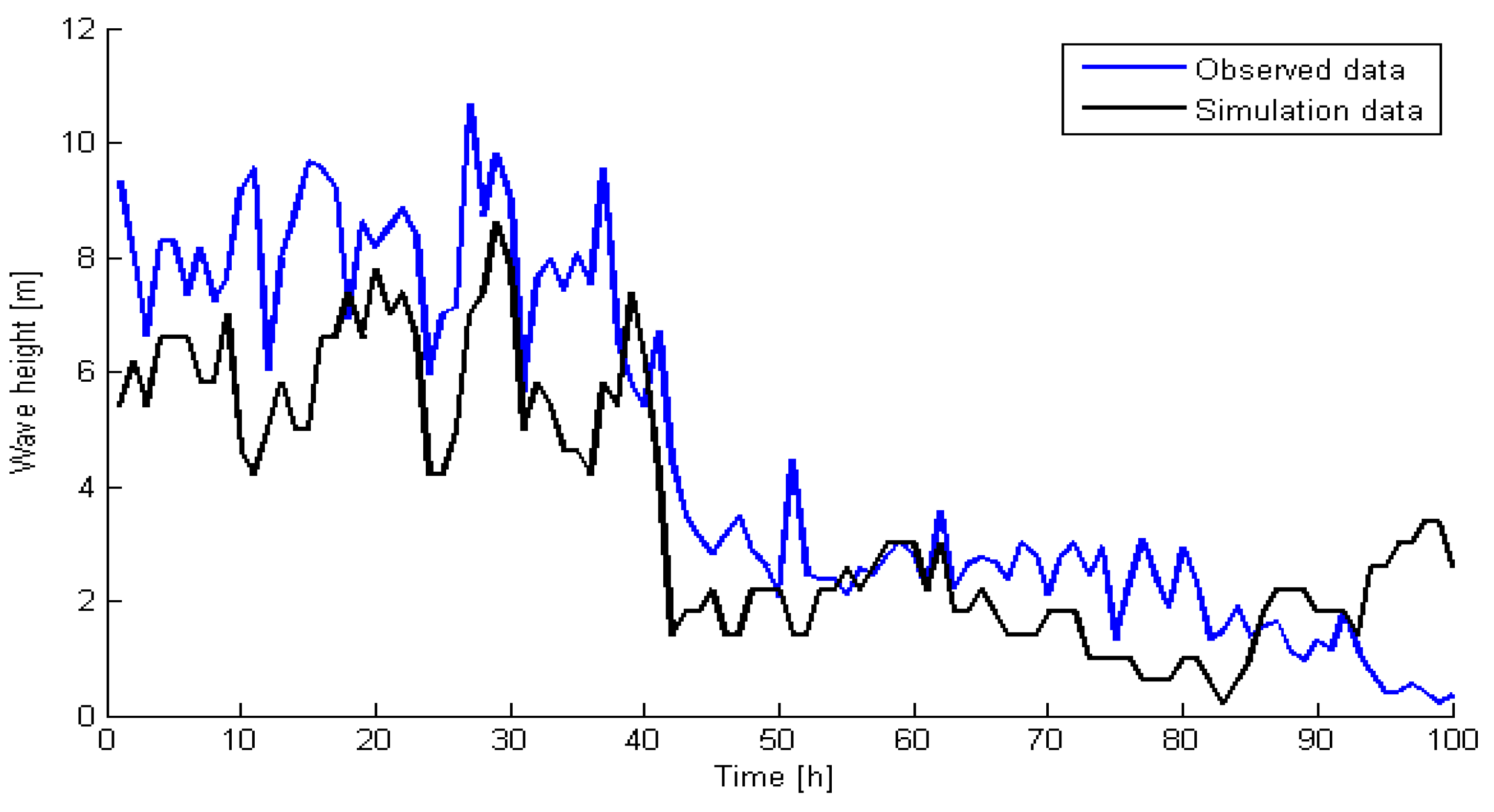
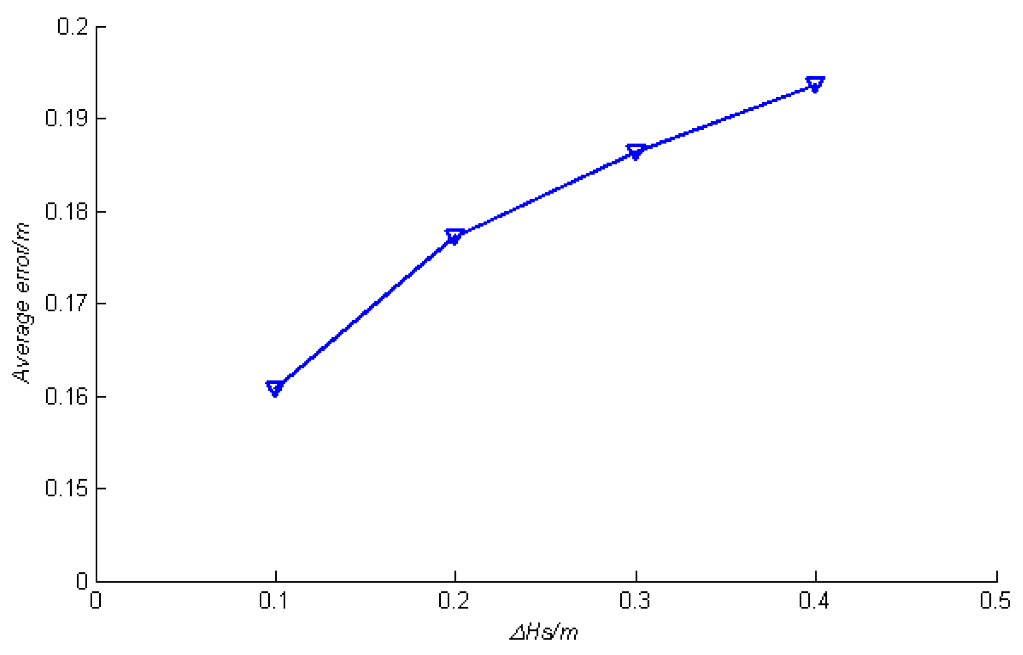
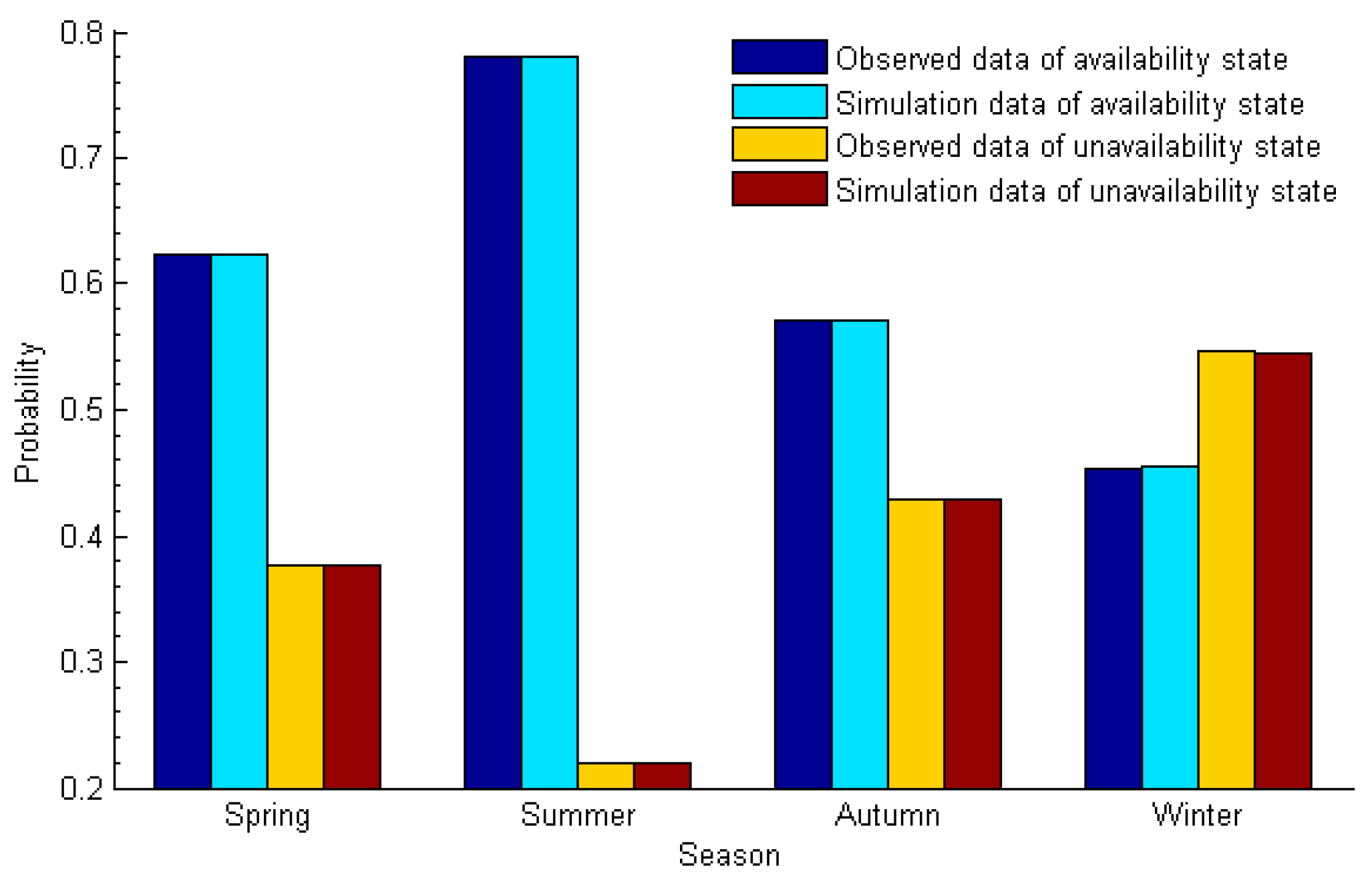
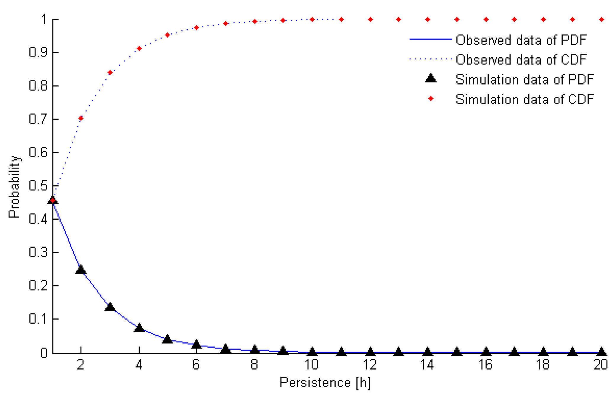
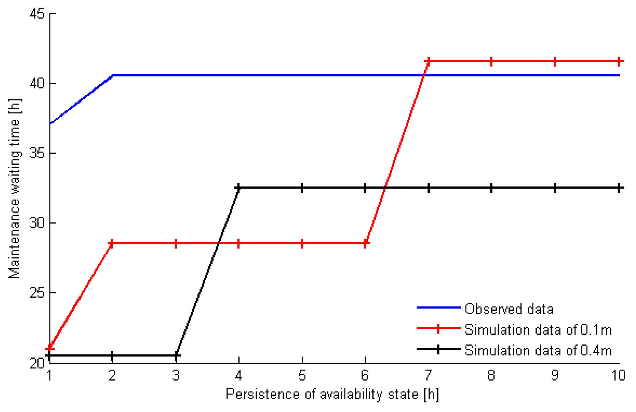
A maintenance waiting time prediction method was introduced for offshore wind turbines. The Markov chain method and dynamic time window were used to describe wind speed and wave height, and a maintenance waiting time prediction model was established. Different to [9], the impacts on maintenance waiting time arising from wind speed and wave height were considered in this paper. The results show that the deviation of the predicted value of the wave height obtained by grouping interval with ∆H_s = 0.1 m was the smallest, which was close to the true value;

(3)

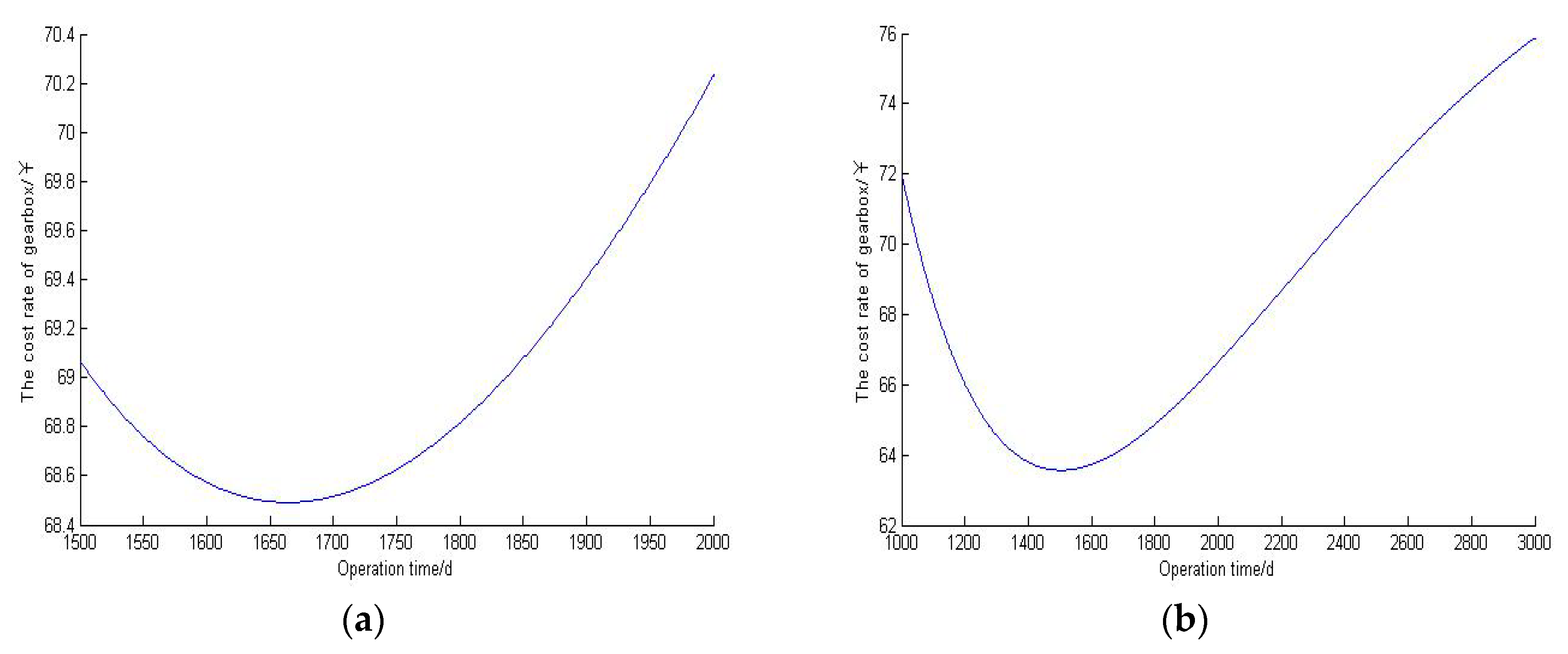
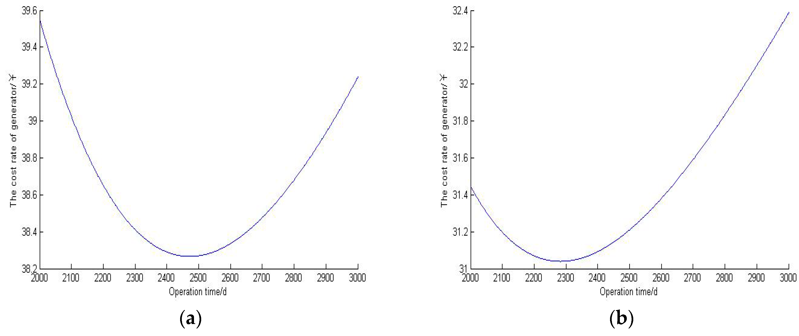
Combining failure maintenance and preventive maintenance, an opportunistic maintenance strategy was presented for offshore wind turbines. The minimum expected maintenance cost was regarded as an objective function to optimize the opportunistic maintenance time and preventive maintenance time. Compared with [10], the opportunistic maintenance strategy reduces maintenance duration and decreases the maintenance waiting time and downtime, thereby reducing maintenance costs. The results show that the maintenance cost was reduced by 10% under the opportunistic maintenance strategy for offshore wind turbine maintenance, which verified the effectiveness and superiority of the opportunistic maintenance strategy for offshore wind turbine maintenance.

References

1. Mahmood, S. Maintenance logistics organization for offshore wind energy: Current progress and future perspectives. Renew. Energy 2015, 77, 182–193. [Google Scholar]
2. Li, X.; Liang, N.; Cheng, Z.J. Estimation of fatigue failure of asphalt concrete based on three-parameter Weibull distribution. Chongqing Jiaotong Univ. (Nat. Sci.) 2017, 1, 178. [Google Scholar]
3. Sanni, S.S.; Chukwu, W.I.E. Inventory model with three-parameter Weibull deterioration, quadratic demand rate and shortages. Am. J. Math. Manag. Sci. 2016, 35, 159. [Google Scholar] [CrossRef]
4. Deng, B.; Jiang, D.; Gong, J. Is a three-parameter Weibull function really necessary for the characterization of the statistical variation of the strength of brittle ceramics? Eur. Ceram. Soc. 2017, 20, 123. [Google Scholar] [CrossRef]
5. Chaurasiya, P.K.; Ahmed, S.; Warudkar, V. Study of different parameters estimation methods of Weibull distribution to determine wind power density using ground based Doppler SODAR instrument. Alex. Eng. J. 2017, 37, 140. [Google Scholar] [CrossRef]
6. Chai, H.; Shin, J.; Lim, T.; Trans, J. Failure rate calculation using the mixture Weibull distribution. Kim. Korean Inst. Electr. Eng. 2017, 66, 500. [Google Scholar]
7. Xu, X.L. Statistical inference for incomplete data three-parameter Weibull distribution. Shanghai Teachers Univ. (Nat. Sci.) 2002, 31, 22. [Google Scholar]
8. Fu, Y.; Xu, W.X.; Liu, L.J. An opportunistic maintenance strategy for offshore wind turbine based on accessibility evaluation. electric power. Wind Eng. 2016, 49, 74–80. [Google Scholar]
9. Liu, L.J.; Fu, Y.; Ma, S.W. Preventive maintenance strategy for offshore wind turbine based on reliability and maintenance priority. Proc. CSEE 2016, 36, 5732–5740. [Google Scholar]
10. Zheng, X.X.; Zhao, H.; Liu, L.J. A Combined maintenance strategy for offshore wind turbine considering accessibility. Power Syst. Technol. 2014, 38, 3030–3036. [Google Scholar]
11. Pedro, G.L.; Luis, V.T.; Matthias, W. Normal behaviour models for wind turbine vibrations: Comparison of neural networks and a stochastic approach. Energies 2017, 10, 1944–1957. [Google Scholar]
12. Pedro, G.L.; Iván, H.; Matthias, W. Fatigue load estimation through a simple stochastic model. Energies 2014, 7, 8279–8293. [Google Scholar]
13. Monbet, V.; Aillot, P.; Prevosto, M. Survey of stochastic models for wind and sea state time series. Probab. Eng. Mech. 2007, 22, 113–126. [Google Scholar] [CrossRef]
14. Matha, D.; Scheu, M.; Muskulus, M. Validation of a Markov-based weather model for simulation of O&M for offshore wind farms. In Proceedings of the 22th International Offshore and Polar Engineering Conference, Rhodes, Greece, 17–22 June 2012; pp. 463–468. [Google Scholar]
15. Scheu, M.; Matha, D.; Hofmann, M.; Muskulus, M. Maintenance strategies for large offshore wind farms. Eng. Proc. 2012, 24, 281–288. [Google Scholar] [CrossRef]
16. Zhang, C.; Gao, W.; Guo, S.; Li, Y.L.; Yang, T. Opportunistic maintenance for wind turbines considering imperfect, reliability-based maintenance. Renew. Energy 2017, 103, 606–612. [Google Scholar] [CrossRef]
17. Mahmood, S.; Maxim, F.; Christophe, B. An opportunistic condition-based maintenance policy for offshore wind turbine blades subjected to degradation and environmental shocks. Reliab. Eng. Syst. Saf. 2015, 142, 463–471. [Google Scholar]
18. Hadi, A.; Karim, A.; Morteza, A. Multi-objective opportunistic maintenance optimization of a wind farm considering limited number of maintenance groups. Renew. Energy 2016, 88, 247–261. [Google Scholar]
19. Ding, F.F.; Tian, Z.G. Opportunistic maintenance for wind farms considering multi-level imperfect maintenance thresholds. Renew. Energy 2012, 45, 175–182. [Google Scholar] [CrossRef]
20. Atashgar, K.; Abdollahzadeh, H. Reliability optimization of wind farms considering redundancy and opportunistic maintenance strategy. Energy Convers. Manag. 2016, 112, 445–458. [Google Scholar] [CrossRef]
21. Hallinan, A.J. A review of the Weibull distribution. Qual. J. Technol. 1993, 25, 85–93. [Google Scholar] [CrossRef]
22. Zhu, W.Y. Design of Mechanical Reliability; Press of Shanghai Jiaotong University: Shanghai, China, 1992; pp. 62–66. [Google Scholar]
23. Zhu, Y.H.; Tai, S.C.; Sun, Y.Y. Applied Mathematical Statistics; Press of Wuhan University of Hydraulic and Electrical Engineering: Wuhan, China, 1999; pp. 68–72. [Google Scholar]
24. Lu, D.J. Stochastic Processes and Applications; Tsinghua Press: Beijing, China, 1986; pp. 100–115. [Google Scholar]
25. Liu, C.H. Stochastic Processes; Press of Huazhong University of Science and Technology: Wuhan, China, 2008; pp. 42–45. [Google Scholar]
26. Liu, Y.F. Research on Reliability of Software System Based on Markov Chain Method; Changchun University of Science and Technology: Changchun, China, 2005. [Google Scholar]
27. Sheldon, M.R. Stochastic Processes, 2nd ed.; John Wiley and Sons: Hoboken, NJ, USA, 1996. [Google Scholar]
28. Qian, M.P. Application on Stochastic Processes; Peking University Press: Beijing, China, 1998. [Google Scholar]
29. Luo, J.Y. Economic Statistical Analysis Methods and Forecasts; Tsinghua Press: Beijing, China, 1987; pp. 347–348. [Google Scholar]
30. Van Bussel, G.J.W.; Zaaijer, M.B. Reliability, availability and maintenance aspects of large-scale offshore wind farms, a concepts study. In Proceedings of the MAREC, Newcastle, UK, 17–18 April 2001; pp. 5–9. [Google Scholar]
31. Hagen, B.; Simonsen, I.; Hofmann, M.; Muskulus, M. A multivariate Markov weather model for O&M simulation of offshore wind parks. Energy Procedia 2013, 35, 137–147. [Google Scholar]
32. Lyding, P.; Faulstich, S.; Hahn, B. Reliability of the electrical parts of wind energy systems-a statistical evaluation of practical experiences. In Proceedings of the EPE Wind Energy Chapter Symposium, Staffordshire University, Stafford, UK, 15–16 April 2010. [Google Scholar]
33. Feng, W.B.; Peng, X.L.; Zhang, S.L. Analysis on wave condition of south ocean of China: No 14. In Proceedings of the China Ocean Science and Technology Symposium, Hohhot, China, 16–17 May 2009. [Google Scholar]
34. Sinha, Y.; Steel, J.A. A progressive study into offshore wind farm maintenance optimization using risk based failure analysis. Renew. Sust. Energ. Rev. 2015, 42, 735–742. [Google Scholar] [CrossRef]
Figure 1. Correlation coefficient method.
Energies 12 02650 g001
Figure 2. Failure-rate curves of Weibull distributions. (a) Comparison of failure rate for three- and two-parameter Weibull distributions. (b) Partial enlarged drawing of maximum likelihood estimation and least-squares estimation.
Energies 12 02650 g002
Figure 3. Preventive maintenance strategy based on age.
Energies 12 02650 g003
Figure 4. The cost rate of blade maintenance based on two- and three-parameter Weibull: the left-hand side (a) shows the blade maintenance cost rate of the two-parameter Weibull, and the right-hand side (b) shows the three-parameter Weibull.
Energies 12 02650 g004
Figure 5. The cost rate of gearbox maintenance based on two- and three-parameter Weibull: the left-hand side (a) shows the gearbox maintenance cost rate of the two-parameter Weibull, and the right-hand side (b) shows the three-parameter Weibull.
Energies 12 02650 g005
Figure 6. The cost rate of generator maintenance based on two- and three-parameter Weibull, the left figure (a) shows the generator maintenance cost rate of the two-parameter Weibull, and the right figure (b) shows the three-parameter Weibull.
Energies 12 02650 g006
Figure 7. Opportunistic maintenance strategy.
Energies 12 02650 g007
Figure 8. The comparison of predicted and observed values of wave height, wave height prediction curve with ∆Hs = 0.1 m.
Energies 12 02650 g008
Figure 9. The comparison of predicted and observed values of wave height, wave height prediction curve with ∆Hs = 0.2 m.
Energies 12 02650 g009
Figure 10. The comparison of predicted and observed values of wave height, wave height prediction curve with ∆Hs = 0.3 m.
Energies 12 02650 g010
Figure 11. The comparison of predicted and observed values of wave height, wave height prediction curve with ∆Hs = 0.4 m.
Energies 12 02650 g011
Figure 12. The average error of the wave height prediction data with ∆Hs = 0.1 m, 0.2 m, 0.3 m, 0.4 m.
Energies 12 02650 g012
Figure 13. The probability of each state occurring in different seasons.
Energies 12 02650 g013
Figure 14. The duration prediction of state H ˜ .
Energies 12 02650 g014
Figure 15. Maintenance waiting time and duration diagram.
Energies 12 02650 g015