Abstract
Machine learning has been applied successfully for faulty wafer detection tasks in semiconductor manufacturing. For the tasks, prediction models are built with prior data to predict the quality of future wafers as a function of their precedent process parameters and measurements. In real-world problems, it is common for the data to have a portion of input variables that are irrelevant to the prediction of an output variable. The inclusion of many irrelevant variables negatively affects the performance of prediction models. Typically, prediction models learned by different learning algorithms exhibit different sensitivities with regard to irrelevant variables. Algorithms with low sensitivities are preferred as a first trial for building prediction models, whereas a variable selection procedure is necessarily considered for highly sensitive algorithms. In this study, we investigate the effect of irrelevant variables on three well-known representative learning algorithms that can be applied to both classification and regression tasks: artificial neural network, decision tree (DT), and k-nearest neighbors (k-NN). We analyze the characteristics of these learning algorithms in the presence of irrelevant variables with different model complexity settings. An empirical analysis is performed using real-world datasets collected from a semiconductor manufacturer to examine how the number of irrelevant variables affects the behavior of prediction models trained with different learning algorithms and model complexity settings. The results indicate that the prediction accuracy of k-NN is highly degraded, whereas DT demonstrates the highest robustness in the presence of many irrelevant variables. In addition, a higher model complexity of learning algorithms leads to a higher sensitivity to irrelevant variables.
1. Introduction
In the semiconductor manufacturing process, the quality of wafers is affected by various of internal and external factors [1,2]. Thus, wafers are monitored and inspected during each operation step of the manufacturing process. Considerable research efforts have focused on employing machine learning for the early detection of defective wafers [3,4,5,6,7]. Prediction models, which predict the quality of each wafer as a function of precedent process parameters and measurements, are constructed by learning from prior data of the manufacturing process. A faulty wafer detection task can be formulated as a supervised learning task. If the task is formulated to predict whether a wafer is faulty, it is called a classification task. A task that predicts continuous-valued quality indicators for each wafer is referred to as a regression task.
A formal setup of a supervised learning task aims to infer an underlying functional relationship of data as a function of input variables to predict output variables. In the training procedure, a learning algorithm is employed to build a function that best approximates the true function f, called a prediction model , from a set of given instances called a training dataset , where is a vector of input variables, is the corresponding value of a output variable, and n is the number of training instances. Determining that is closest to f is crucial for obtaining high prediction accuracy, which is primarily determined by both the dataset and the learning algorithm used.
Practically, only a few input variables are usually observed to be relevant to the output variable. Therefore, several irrelevant variables appear in a dataset [8,9]. Relevant variables contribute to the improvement of prediction accuracy based on their degree of relevance. However, irrelevant variables do not, and they may even negatively affect the prediction accuracy [10]. If a prediction model that depends excessively on irrelevant variables is built, it will not perform well in future instances [11]. Moreover, the inclusion of many irrelevant variables may degrade the efficiency of learning algorithms [12,13] and result in misleading interpretations and decision-making [14,15].
When learning with irrelevant variables, one can consider performing variable selection, which aims to select a subset of relevant variables from the entire set of input variables to improve the prediction accuracy [16,17]. By applying a variable selection procedure, we can obtain more accurate and concise prediction models that include a reduced number of input variables. However, this procedure is computationally intensive for high-dimensional datasets containing numerous input variables [18,19,20,21]. When computational time and resources are limited, a single learning algorithm that is less sensitive to irrelevant variables is preferable [9]. This provides good prediction models that can be used as is without requiring variable selection.
In this study, we evaluate the effect of the number of irrelevant variables on different learning algorithms, each of which builds a prediction model in a different manner based on its own competence. We analyze the characteristics of three representative and widely used learning algorithms that can be applied to both classification and regression problems: artificial neural network (ANN), decision tree (DT), and k-nearest neighbors (k-NN). We further investigate for each learning algorithm that how the model complexity affects the sensitivity to irrelevant variables. The different behaviors of prediction models trained with various conditions are demonstrated through an empirical study using real-world datasets collected from a semiconductor manufacturer based in the Republic of Korea.
The remainder of this paper is organized as follows. In Section 2, an overview of the related work is presented. In Section 3, an analysis of the characteristics of the learning algorithms in the presence of irrelevant variables is presented. In Section 4, the results of the empirical investigations are reported. Finally, conclusions and practical guidelines are discussed in Section 5.
2. Related Work
For supervised learning tasks, we often encounter real-world problems with high-dimensional datasets containing numerous input variables. It is important to determine which variables to use and which to ignore when predicting output variables for unknown novel instances [9]. Various learning algorithms are available for building prediction models from data. They demonstrate different sensitivities to irrelevant variables [14,22,23,24,25]. Some learning algorithms attempt to directly reflect each variable’s relevance or automatically discard irrelevant ones based on their intrinsic characteristics. In contrast, some are vulnerable to the presence of irrelevant variables.
To achieve superior prediction accuracy for those datasets expected to contain many irrelevant variables, we would prefer using only those input variables that are relevant to the output variables in order to ciaviod any negative effects caused by irrelevant variables. Ideally, it is desirable to find the subset of input variables yielding the best prediction accuracy [8]. An exhaustive comparison of every possible subset is computationally impractical [26]. Therefore, variable selection has been an important research topic to develop an optimal variable subset efficiently. Notably, variable selection is distinct from feature extraction, which constructs new variables by combining the original input variables, e.g., principal component analysis [27].
Considerable research efforts have been devoted to the development of various variable selection methods, which are mainly categorized into filter and wrapper approaches [16,17]. The filter approach uses proxy measures to evaluate the relevance of individual variables based on data properties. The filter approach is computationally efficient but usually yields lower prediction accuracy than the wrapper approach. Recent studies on this approach have focused on maximizing variable relevancy while minimizing variable redundancy based on information theory [28,29,30]. The wrapper approach evaluates variable subsets by building prediction models directly on the subsets using a learning algorithm [31]. For the wrapper approach, sequential methods, which add or remove variables sequentially to maximize the prediction accuracy, have been studied. More recent studies on this approach have often used stochastic methods which are based on meta-heuristics, such as genetic algorithm [32,33,34], particle swarm optimization [35,36,37], simulated annealing [38], and ant colony optimization [39]. Stochastic methods have successfully exhibited superior performance, but they suffer from high computational cost. Some studies have compared existing variable selection methods in terms of the prediction accuracy on various real-world applications, such as medical classification [40], object classification [41], and link prediction [42].
Although previous studies have focused mainly on variable selection approaches, these approaches are computationally too expensive [18,19] and introduce a high risk of overfitting [20,21] especially for high-dimensional datasets. With limited computational time and resources, we must develop an efficient means based on the characteristics of each learning algorithm with respect to irrelevant variables. For learning algorithms that are highly sensitive to irrelevant variables, variable selection would be necessary. On the other hand, variable selection would be unnecessary for less sensitive learning algorithms [9]. Thus, less sensitive learning algorithms without variable selection would be preferable in terms of efficiency. To this end, aiming to provide practical guidelines for learning with irrelevant variables, this study analyzes and empirically examines the effect of irrelevant variables on the three representative learning algorithms.
3. Learning with Irrelevant Variables
In this study, the effect of irrelevant variables on the accuracy of different prediction models is examined. The prediction models are trained using ANN, DT, and k-NN. These learning algorithms can be applied to both classification and regression tasks, and they have widely been used for various real-world applications [43,44,45,46,47]. Both high and low model complexity settings for each of these algorithms are considered, as model complexity is adjustable by modifying their hyperparameter settings. It should be noted that model complexity indicates how well a model fits underlying data distributions. A low-complexity model fits only a few specific data distributions, whereas a high-complexity model fits almost all data distributions. The following subsections briefly introduce the learning algorithms and analyze the effect of irrelevant variables considering different model complexities.
3.1. Artificial Neural Network (ANN)
ANN is based on a collection of connected units organized in a sequence of layers, inspired by biological neural networks in the brain. In this study, the feed-forward neural network architecture consisting of input, hidden, and output layers is considered. The layers are sequentially connected through linear combinations of non-linear functions. The units of the input layer transmit input variables to the units of the hidden layer. At the hidden layer, the feature vector with respect to is obtained as , where is the weight matrix from the input layer to the hidden layer, is the bias vector of the hidden layer, and is a non-linear activation function, e.g., logistic sigmoid function. Subsequently, the output layer produces the prediction results for the output variable. The prediction for y is of the functional form , where is the weight matrix from the hidden layer to the output layer and is the bias vector of the output layer. The output function o depends on the target task, for which sigmoid and linear functions are typically used in classification and regression tasks, respectively. Given the training set , the prediction model f for ANN is trained by minimizing the error function with respect to the component weights and biases through backpropagation, where L is the loss function. The popular choice of L is the cross entropy for the classification task and the mean squared error for the regression task.
The model complexity for the ANN is determined by the number of hidden layers and the number of hidden units in the hidden layers of the prediction model, as an increase in these hyperparameters results in a greater number of adjustable weights during the training [48,49,50]. In this study, a model architecture with only one hidden layer is considered, and model complexity is controlled by adjusting only the number of hidden units. A greater number of hidden units indicates a higher model complexity.
In the presence of irrelevant variables, the ANN reduces the effect of irrelevant variables on the prediction model by optimizing weights during the training. However, non-zero values are inherently assigned to weights of every pair of input and hidden units including those corresponding to irrelevant variables. As the weights for irrelevant variables add noise to the prediction results, they negatively affect the prediction accuracy [51]. Moreover, the inclusion of more irrelevant variables increases the number of local optima in the error function, because there are more combinations of weights that can yield locally optimal values of the error function [52]. This can become a serious problem as more hidden units are used in the prediction model, which increases model complexity.
3.2. Decision Tree (DT)
DT induces a hierarchical structure of several nodes, each of which is in the form of an if-then-else decision rule. During the training, node splits are performed through recursive partitioning of the training set , where each node split is performed by selecting the input variable that best discriminates the output values of training instances in the current node. The prediction model is defined as sequences of induced rules such that each test instance is assigned to one leaf node in the model. The output value for is predicted based on training instances satisfying the corresponding rules, and the mode and mean of the output values for these instances are used for the classification and regression tasks, respectively. The prediction logic of the model is easy to understand and interpret.
The DT has a higher model complexity as the size of the prediction model increases with an increase in the depth of the node hierarchy and a decrease in the minimum allowable size of each leaf node [53].
The recursive partitioning for the DT can be regarded as an embedded variable selection procedure, as a few relevant variables are used for node splits whereas most irrelevant variables are automatically discarded during the procedure. Owing to this property, DT has been known to be more robust to irrelevant variables compared with other learning algorithms. In the presence of many irrelevant variables, however, there is an increased likelihood of spurious node splits occurring on some irrelevant variables during the training [14]. A prediction model with a higher model complexity is more likely to contain many spurious node splits, which may degrade the prediction accuracy [22].
3.3. k-Nearest Neighbors (k-NN)
k-NN is an instance-based learning algorithm that simply stores training instances without model training before making predictions. This algorithm assumes that the output of an instance is similar to those of its nearest neighbors. For each test instance , it simply finds the k training instances closest to in terms of a pre-determined distance measure, e.g., Euclidean distance. Prediction is performed by aggregating the output values of the selected k instances depending on the target task. For simplicity of description, let denote the selected instance with respect to . For the classification task, the prediction model f is defined by majority voting of output values as . For the regression task, it can typically be defined by an average of output values such that .
For the k-NN, the number of neighbors k is inversely related to model complexity. With a small k, the prediction model concentrates more on, and is thus more sensitive to the local structures in data. In contrast, for a large k, the prediction model captures the global structure of data.
It is well-known that the prediction accuracy of the k-NN is highly sensitive to irrelevant variables, because the distance measure potentially misrepresents the neighborhood information between instances with the presence of irrelevant variables [23,24]. If there are many more irrelevant variables than relevant ones, the distance measure tends to become uninformative. Accordingly, the nearest neighbors selected by the k-NN will not be the actual neighbors, thereby resulting in misleading prediction [25]. Moreover, for an extremely small k, the prediction accuracy is further degraded, as the output value for a test instance is more likely to be predicted using only a few non-neighbor training instances.
4. Empirical Analysis
An empirical analysis is conducted for faulty wafer detection tasks using real-world datasets to demonstrate the different behaviors of prediction models trained by different learning algorithms with various conditions in terms of the number of irrelevant variables and model complexity.
4.1. Problem Description
For the empirical analysis, we conduct a case study using two real-world datasets from a semiconductor manufacturer based in the Republic of Korea. The two datasets were collected over a period of 7.5 months from the photolithography process in semiconductor wafer fabrication. In the data collection environment, wafers are processed by photolithography equipment, and subsequently, are inspected by metrology equipment to assess their quality. The two datasets, each corresponding to different photolithography equipment (EQ1, EQ2), contain 2583 and 2509 wafer records, respectively. The number of input and output variables for the datasets are 102 and 4, respectively. The input variables comprise various process sensor measurements (e.g., heating temperature, exposure duration and mask overlay) from the photolithography equipment and summary statistics from the previous metrology equipment. All the input variables are standardized to have a mean of 0 and a standard deviation of 1. The output variables comprise four continuous-valued quality indicators from the subsequent metrology equipment, which are related to overlay misalignment. For the j-th output variable , a specification of its target range is given in the form of , where is an upper limit. A wafer is regarded as faulty with respect to the j-th output variable if the value of lies outside the corresponding target range. We define the binarized output variables as , each of which indicates whether a wafer is faulty with respect to the j-th output variable. For faulty wafer detection as a classification task, the prediction models are built to predict the binary output variables . For detection as a regression task, the prediction models predict the continuous output variables . The details of the datasets are listed in Table 1. It should be noted that all the datasets are highly imbalanced with low rates of faulty wafers.

Table 1.
Details of datasets used in experiments.
4.2. Experimental Design
For the empirical analysis, six types of prediction models based on combinations of three learning algorithms (ANN, DT, and k-NN) and two model complexity settings (high and low) were considered for the classification and regression tasks. The model complexity for the learning algorithms was adjusted based on individual hyperparameters, as described in Section 3. The detailed settings for the six types of prediction models are listed in Table 2.
Table 2.
Prediction models and their settings.
To demonstrate the effect of irrelevant variables on the prediction accuracy of various prediction models, irrelevant variables containing random numbers from the standard normal distribution were generated for use as artificial input variables. As the baselines, prediction models trained only with the original input variables were used. To evaluate the effect of an increase in the number of irrelevant variables on prediction accuracy, varying numbers of artificial input variables were added to the dataset to build the prediction models. All models were implemented using the scikit-learn library in Python [54]. For the classification tasks, we used neural_network.MLPClassifier, tree.DecisionTreeClassifier, and neighbors.KNeighborsClassifier functions to implement ANN, DT, and k-NN, respectively. For the regression tasks, neural_network.MLPRegressor, tree.DecisionTreeRegressor, and neighbors.KNeighborsRegressor functions were used for ANN, DT, and k-NN, respectively.
The performance of the prediction models for faulty wafer detection tasks were evaluated through a five-fold cross validation procedure. In this procedure, the original dataset was partitioned into five disjointed equal-sized subsets. Subsequently, each subset was used exactly once to evaluate the performance, such that four subsets and the remaining subset were used as the training and test sets, respectively. To exclude the dependency of prediction performance on the characteristics in the datasets and learning algorithms, we alternatively evaluated how well each prediction model, which was trained with some artificial irrelevant variables, obtains the predictions by its baseline model on the test set.
The performance was evaluated according to the area under the receiver operating characteristics curve (AUC) [55,56]. The AUC assesses how well a prediction model performs in general, as calculated by unifying various possible settings of the decision threshold for the model. To inducate the performance degradation of the prediction models against the baseline models, the relative AUCs were calculated as the AUC values divided by the baseline AUC. Therefore, the relative AUC for the baseline model was set to 1, and a value smaller than 1 indicates that the performance of the prediction model is worse than that of the baseline. A lower value of the relative AUC indicates a lower prediction performance.
All the experiments were performed 20 times independently, and the results were reported as an average over the 20 runs.
4.3. Results and Discussion
Figure 1a,b plots the relative AUC against the number of artificial irrelevant variables for each prediction model averaged over the different classification tasks on the EQ1 and EQ2 datasets, respectively. Figure 1c,d shows the experimental results for the regression tasks. Overall, the results were consistent with the characteristics of the learning algorithms discussed in Section 3. The relative AUCs of all the prediction models tended to decrease as irrelevant variables were added to the dataset. A higher model complexity resulted in higher sensitivity to irrelevant variables for every learning algorithm.
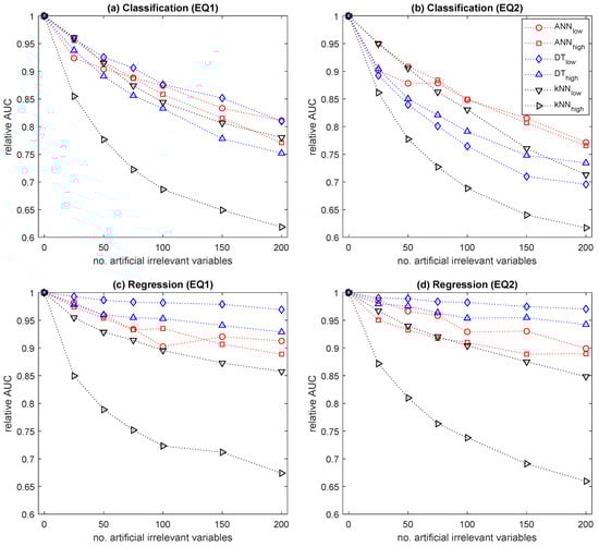
Figure 1.
Effect of irrelevant variables on prediction performance: (a) classification tasks on EQ1 data; (b) classification tasks on EQ2 data; (c) regression tasks on EQ1 data; (d) regression tasks on EQ2 data.
All the models for the classification tasks yielded a substantial decrease in the relative AUC with an increase in the number of irrelevant variables, compared to the models for the regression tasks. However, with many irrelevant variables, learning algorithms were more vulnerable to class imbalance. Under class imbalance situations where there were only a few faulty wafers in the training and validation sets, some artificial irrelevant variables were coincidentally correlated with output variables so that the prediction models would depend largely on those irrelevant variables. This resulted in the degradation of the generalization performance. For the k-NN, as more irrelevant variables were included, relatively non-near neighbors were selected rather than the actual nearest neighbors in the training set for each test instance. Therefore, the output values of the selected training instances differed from those that would be obtained if the actual neighbors had been selected. As the prediction performance for the classification task is determined based on whether each test instance is correctly classified, even a low number of erroneous selections of the nearest neighbors yielded a substantial decrease in the relative AUC, especially when k was small.
Regarding the regression tasks, the DT was the most robust, as it involves an embedded variable selection procedure. The AUC of the DT slightly decreased with the number of irrelevant variables. In contrast, the k-NN was the most vulnerable to irrelevant variables, as the distance measure reflected the actual neighborhood information in data to a lesser extent with the addition of irrelevant variables. The performance of the k-NN was greatly degraded in the presence of many irrelevant variables.
Without considering the absolute degree of prediction performance, the DT would be the preferred learning algorithm when the given dataset is expected to include many irrelevant variables, and the ANN would the next best choice. In addition, using lower-complexity prediction models would be preferred to address this type of dataset. On the other hand, applying variable selection is essential for prediction models that are sensitive to irrelevant variables, particularly for the k-NN with a high model complexity, which is very sensitive to irrelevant variables.
5. Concluding Remarks
In this study, the effect of irrelevant variables on faulty wafer detection tasks with ANN, DT, and k-NN was investigated. We analyzed the characteristics of each learning algorithm with respect to the number of irrelevant variables and the model complexity. For the classification and regression tasks, we empirically examined the behaviors of prediction models trained by each learning algorithm under various conditions in terms of the number of irrelevant variables and the model complexity.
From the empirical study, it was observed that the inclusion of irrelevant variables negatively affected the prediction accuracy for every prediction model. With many irrelevant variables, the prediction accuracy of the k-NN was highly degraded. The DT demonstrated the best robustness to irrelevant variables for the regression tasks, whereas it was relatively less robust for the classification tasks. A higher model complexity of the learning algorithms induced a higher sensitivity to irrelevant variables. Subsequently, variable selection must be considered if learning algorithms sensitive to irrelevant variables are employed. In contrast, less sensitive learning algorithms do not require the use of a variable selection procedure.
The above conclusions serve as a guideline for practitioners to better address various real-world scenarios of expert and intelligent systems involving learning with many irrelevant variables. Without any constraints, we can conduct extensive comparisons of numerous available prediction models trained by different learning algorithms by simultaneously considering variable selection and hyperparameter optimization for each model. Extensive comparisons are intractable in cases where the prediction models should be re-trained owing to changes in data characteristics with time and where the learning tasks are subjected to practical time and resource constraints. Accordingly, the use of a single learning algorithm that is insensitive to irrelevant variables would be a reasonable choice.
We focused on analyzing the effect of irrelevant variables on faulty wafer detection tasks. One limitation is that the effects of other data characteristics, which differ from dataset to dataset and would significantly affect the behavior of a learning algorithm, were not analyzed in this study. In future work, we will consider a meta-learning framework to investigate various other data characteristics further.
Author Contributions
Conceptualization, D.K. and S.K.; methodology, D.K.; validation, S.K.; writing—original draft preparation, D.K.; writing—review and editing, S.K.
Funding
This work was supported by the National Research Foundation of Korea (NRF) grant funded by the Korea government (MSIT; Ministry of Science and ICT) (No. NRF-2017R1C1B5075685). This work was also supported by research fund of Chungnam National University.
Conflicts of Interest
The authors declare no conflict of interest.
References
- Su, A.J.; Jeng, J.C.; Huang, H.P.; Yu, C.C.; Hung, S.Y.; Chao, C.K. Control relevant issues in semiconductor manufacturing: Overview with some new results. Control. Eng. Pract. 2007, 15, 1268–1279. [Google Scholar] [CrossRef]
- Uzsoy, R.; Lee, C.Y.; Martin-Vega, L.A. A review of production planning and scheduling models in the semiconductor industry part I: System characteristics, performance evaluation and production planning. IIE Trans. 1992, 24, 47–60. [Google Scholar] [CrossRef]
- Chen, P.; Wu, S.; Lin, J.; Ko, F.; Lo, H.; Wang, J.; Yu, C.H.; Liang, M.S. Virtual metrology: A solution for wafer to wafer advanced process control. In Proceedings of the 2005 IEEE International Symposium on Semiconductor Manufacturing, San Jose, CA, USA, 13–15 September 2005; pp. 155–157. [Google Scholar]
- Yung-Cheng, J.C.; Cheng, F.T. Application development of virtual metrology in semiconductor industry. In Proceedings of the 32nd Annual Conference of IEEE Industrial Electronics Society, Raleigh, NC, USA, 6–10 November 2005; pp. 124–129. [Google Scholar]
- Kim, D.; Kang, P.; Cho, S.; Lee, H.-j.; Doh, S. Machine learning-based novelty detection for faulty wafer detection in semiconductor manufacturing. Expert Syst. Appl. 2012, 39, 4075–4083. [Google Scholar] [CrossRef]
- He, Q.P.; Wang, J. Fault detection using the k-nearest neighbor rule for semiconductor manufacturing processes. IEEE Trans. Semicond. Manuf. 2007, 20, 345–354. [Google Scholar] [CrossRef]
- Chien, C.F.; Hsu, C.Y.; Chen, P.N. Semiconductor fault detection and classification for yield enhancement and manufacturing intelligence. Flex. Serv. Manuf. J. 2013, 25, 367–388. [Google Scholar] [CrossRef]
- John, G.H.; Kohavi, R.; Pfleger, K. Irrelevant features and the subset selection problem. In Proceedings of the 11th International Conference on Machine Learning, New Brunswick, NJ, USA, 10–13 July 1994; pp. 121–129. [Google Scholar]
- Langley, P. Selection of relevant features in machine learning. In Proceedings of the 1994 AAAI Fall Symposium on Relevance, New Orleans, LA, USA, 4–6 November 1994; Volume 184, pp. 245–271. [Google Scholar]
- Abdullah, S.; Sabar, N.R.; Nazri, M.Z.A.; Ayob, M. An Exponential Monte-Carlo algorithm for feature selection problems. Comput. Ind. Eng. 2014, 67, 160–167. [Google Scholar] [CrossRef]
- Kotsiantis, S.B. Decision trees: A recent overview. Artif. Intell. Rev. 2013, 39, 261–283. [Google Scholar] [CrossRef]
- Fomby, T.B. Loss of efficiency in regression analysis due to irrelevant variables: A generalization. Econ. Lett. 1981, 7, 319–322. [Google Scholar] [CrossRef]
- Dhagat, A.; Hellerstein, L. PAC learning with irrelevant attributes. In Proceedings of the 35th Annual Symposium on Foundations of Computer Science, Santa Fe, NM, USA, 20–22 November 1994; pp. 64–74. [Google Scholar]
- Loh, W.Y. Fifty years of classification and regression trees. Int. Stat. Rev. 2014, 82, 329–348. [Google Scholar] [CrossRef]
- Goldstein, W.M.; Busemeyer, J.R. The effect of “irrelevant” variables on decision making: Criterion shifts in preferential choice? Organ. Behav. Hum. Decis. Process. 1992, 52, 425–454. [Google Scholar] [CrossRef]
- Chandrashekar, G.; Sahin, F. A survey on feature selection methods. Comput. Electr. Eng. 2014, 40, 16–28. [Google Scholar] [CrossRef]
- Guyon, I.; Elisseeff, A. An introduction to variable and feature selection. J. Mach. Learn. Res. 2003, 3, 1157–1182. [Google Scholar]
- Gheyas, I.A.; Smith, L.S. Feature subset selection in large dimensionality domains. Pattern Recognit. 2010, 43, 5–13. [Google Scholar] [CrossRef]
- Ng, A.Y. On feature selection: Learning with exponentially many irrevelant features as training examples. In Proceedings of the 15th International Conference on Machine Learning, San Francisco, CA, USA, 24–27 July 1998; pp. 404–412. [Google Scholar]
- Jain, A.; Zongker, D. Feature selection: Evaluation, application, and small sample performance. IEEE Trans. Pattern Anal. Mach. Intell. 1997, 19, 153–158. [Google Scholar] [CrossRef]
- Raudys, S.J.; Jain, A.K. Small sample size effects in statistical pattern recognition: Recommendations for practitioners. IEEE Trans. Pattern Anal. Mach. Intell. 1991, 13, 252–264. [Google Scholar] [CrossRef]
- Chang, Y. Variable selection via regression trees in the presence of irrelevant variables. Commun. Stat. Simul. Comput. 2013, 42, 1703–1726. [Google Scholar] [CrossRef]
- Aha, D.W. Tolerating noisy, irrelevant and novel attributes in instance-based learning algorithms. Int. J. Man-Mach. Stud. 1992, 36, 267–287. [Google Scholar] [CrossRef]
- Güvenir, H.A. A classification learning algorithm robust to irrelevant features. In Proceedings of the 8th International Conference on Artificial Intelligence: Methodology, Systems, and Applications, Sozopol, Bulgaria, 21–23 September 1998; pp. 281–290. [Google Scholar]
- Langley, P.; Iba, W. Average-case analysis of a nearest neighbor algorthim. In Proceedings of the 13th International Joint Conference on Artifical Intelligence, Chambery, France, 28 August–3 September 1993; pp. 889–894. [Google Scholar]
- Huang, C.L.; Wang, C.J. A GA-based feature selection and parameters optimization for support vector machines. Expert Syst. Appl. 2006, 31, 231–240. [Google Scholar] [CrossRef]
- Abe, S. Feature selection and extraction. In Support Vector Machines for Pattern Classification; Springer: London, UK, 2010; pp. 331–341. [Google Scholar]
- Gao, W.; Hu, L.; Zhang, P. Class-specific mutual information variation for feature selection. Pattern Recognit. 2018, 79, 328–339. [Google Scholar] [CrossRef]
- Gao, W.; Hu, L.; Zhang, P.; He, J. Feature selection considering the composition of feature relevancy. Pattern Recognit. Lett. 2018, 112, 70–74. [Google Scholar] [CrossRef]
- Macedo, F.; Oliveira, M.R.; Pacheco, A.; Valadas, R. Theoretical foundations of forward feature selection methods based on mutual information. Neurocomputing 2019, 325, 67–89. [Google Scholar] [CrossRef]
- Kang, S.; Kim, D.; Cho, S. Efficient feature selection-based on random forward search for virtual metrology modeling. IEEE Trans. Semicond. Manuf. 2016, 29, 391–398. [Google Scholar] [CrossRef]
- Tao, Z.; Huiling, L.; Wenwen, W.; Xia, Y. GA-SVM based feature selection and parameter optimization in hospitalization expense modeling. Appl. Soft Comput. 2019, 75, 323–332. [Google Scholar] [CrossRef]
- Khammassi, C.; Krichen, S. A GA-LR wrapper approach for feature selection in network intrusion detection. Comput. Secur. 2017, 70, 255–277. [Google Scholar] [CrossRef]
- De Stefano, C.; Fontanella, F.; Marrocco, C.; Di Freca, A.S. A GA-based feature selection approach with an application to handwritten character recognition. Pattern Recognit. Lett. 2014, 35, 130–141. [Google Scholar] [CrossRef]
- Mistry, K.; Zhang, L.; Neoh, S.C.; Lim, C.P.; Fielding, B. A micro-GA embedded PSO feature selection approach to intelligent facial emotion recognition. IEEE Trans. Cybern. 2017, 47, 1496–1509. [Google Scholar] [CrossRef] [PubMed]
- Zhang, Y.; Gong, D.W.; Sun, X.Y.; Guo, Y.N. A PSO-based multi-objective multi-label feature selection method in classification. Sci. Rep. 2017, 7, 376. [Google Scholar] [CrossRef] [PubMed]
- Gu, S.; Cheng, R.; Jin, Y. Feature selection for high-dimensional classification using a competitive swarm optimizer. Soft Comput. 2018, 22, 811–822. [Google Scholar] [CrossRef]
- Mafarja, M.M.; Mirjalili, S. Hybrid Whale Optimization Algorithm with simulated annealing for feature selection. Neurocomputing 2017, 260, 302–312. [Google Scholar] [CrossRef]
- Sweetlin, J.D.; Nehemiah, H.K.; Kannan, A. Feature selection using ant colony optimization with tandem-run recruitment to diagnose bronchitis from CT scan images. Comput. Methods Programs Biomed. 2017, 145, 115–125. [Google Scholar] [CrossRef]
- Sanchez-Pinto, L.N.; Venable, L.R.; Fahrenbach, J.; Churpek, M.M. Comparison of variable selection methods for clinical predictive modeling. Int. J. Med. Inform. 2018, 116, 10–17. [Google Scholar] [CrossRef] [PubMed]
- Ma, L.; Fu, T.; Blaschke, T.; Li, M.; Tiede, D.; Zhou, Z.; Ma, X.; Chen, D. Evaluation of feature selection methods for object-based land cover mapping of unmanned aerial vehicle imagery using random forest and support vector machine classifiers. ISPRS Int. J. Geo-Inf. 2017, 6, 51. [Google Scholar] [CrossRef]
- Pecli, A.; Cavalcanti, M.C.; Goldschmidt, R. Automatic feature selection for supervised learning in link prediction applications: A comparative study. Knowl. Inf. Syst. 2018, 56, 85–121. [Google Scholar] [CrossRef]
- Zidek, K.; Maxim, V.; Pitel, J.; Hosovsky, A. Embedded vision equipment of industrial robot for inline detection of product errors by clustering–classification algorithms. Int. J. Adv. Robot. Syst. 2016, 13, 1729881416664901. [Google Scholar] [CrossRef]
- Kang, P.; Lee, H.J.; Cho, S.; Kim, D.; Park, J.; Park, C.K.; Doh, S. A virtual metrology system for semiconductor manufacturing. Expert Syst. Appl. 2009, 36, 12554–12561. [Google Scholar] [CrossRef]
- Lieber, D.; Stolpe, M.; Konrad, B.; Deuse, J.; Morik, K. Quality prediction in interlinked manufacturing processes based on supervised & unsupervised machine learning. Procedia CIRP 2013, 7, 193–198. [Google Scholar]
- Ngai, E.W.T.; Xiu, L.; Chau, D.C.K. Application of data mining techniques in customer relationship management: A literature review and classification. Expert Syst. Appl. 2009, 36, 2592–2602. [Google Scholar] [CrossRef]
- Köksal, G.; Batmaz, İ.; Testik, M.C. A review of data mining applications for quality improvement in manufacturing industry. Expert Syst. Appl. 2011, 38, 13448–13467. [Google Scholar] [CrossRef]
- Han, S.; Pool, J.; Tran, J.; Dally, W. Learning both weights and connections for efficient neural network. In Proceedings of the 28th International Conference on Neural Information Processing Systems, Montreal, QC, Canada, 7–12 December 2015; pp. 1135–1143. [Google Scholar]
- Sontag, E.D. VC dimension of neural networks. Nato ASI Ser. Comput. Syst. Sci. 1998, 168, 69–96. [Google Scholar]
- Bianchini, M.; Scarselli, F. On the complexity of neural network classifiers: A comparison between shallow and deep architectures. IEEE Trans. Neural Networks Learn. Syst. 2014, 25, 1553–1565. [Google Scholar] [CrossRef]
- May, R.J.; Maier, H.R.; Dandy, G.C.; Fernando, T.M.K.G. Non-linear variable selection for artificial neural networks using partial mutual information. Environ. Model. Softw. 2008, 23, 1312–1326. [Google Scholar] [CrossRef]
- Suzuki, K. Artificial Neural Networks—Methodological Advances and Biomedical Applications; InTech: Temse, Belgium, 2011. [Google Scholar]
- Mingers, J. An empirical comparison of pruning methods for decision tree induction. Mach. Learn. 1989, 4, 227–243. [Google Scholar] [CrossRef]
- Pedregosa, F.; Varoquaux, G.; Gramfort, A.; Michel, V.; Thirion, B.; Grisel, O.; Blondel, M.; Prettenhofer, P.; Weiss, R.; Dubourg, V.; et al. Scikit-learn: machine Learning in Python. J. Mach. Learn. Res. 2011, 12, 2825–2830. [Google Scholar]
- Bradley, A.P. The use of the area under the ROC curve in the evaluation of machine learning algorithms. Pattern Recognit. 1997, 30, 1145–1159. [Google Scholar] [CrossRef]
- Huang, J.; Ling, C.X. Using AUC and accuracy in evaluating learning algorithms. IEEE Trans. Knowl. Data Eng. 2005, 17, 299–310. [Google Scholar] [CrossRef]

© 2019 by the authors. Licensee MDPI, Basel, Switzerland. This article is an open access article distributed under the terms and conditions of the Creative Commons Attribution (CC BY) license (http://creativecommons.org/licenses/by/4.0/).