Article

Machine Learning-Based Soft Sensors for the Estimation of Laundry Moisture Content in Household Dryer Appliances

by
Giuliano Zambonin
1,2,*,
Fabio Altinier
2,
Alessandro Beghi
1,
Leandro dos Santos Coelho
3,4,
Nicola Fiorella
1,
Terenzio Girotto
2,
Mirco Rampazzo
1,
Gilberto Reynoso-Meza
3 and
Gian Antonio Susto
1
1
Department of Information Engineering, University of Padova, 35131 Padova, Italy
2
Electrolux Italia S.p.a, 33080 Porcia (PN), Italy
3
Industrial and Systems Engineering Graduate Program (PPGEPS), Pontificia Universidade Católica do Paraná (PUCPR), Curitiba (PR) 80215-901, Brazil
4
Department of Electrical Engineering, Federal University of Paraná (UFPR), Curitiba (PR) 80060-000, Brazil
*
Author to whom correspondence should be addressed.
Energies 2019, 12(20), 3843; https://doi.org/10.3390/en12203843
Submission received: 8 September 2019 / Revised: 27 September 2019 / Accepted: 8 October 2019 / Published: 11 October 2019
(This article belongs to the Special Issue Advanced Manufacturing Informatics, Energy and Sustainability)

Abstract

:
The aim is to develop soft sensors (SSs) to provide an estimation of the laundry moisture of clothes introduced in a household Heat Pump Washer–Dryer (WD-HP) appliance. The developed SS represents a cost-effective alternative to physical sensors, and it aims at improving the WD-HP performance in terms of drying process efficiency of the automatic drying cycle. To this end, we make use of appropriate Machine Learning models, which are derived by means of Regularization and Symbolic Regression methods. These methods connect easy-to-measure variables with the laundry moisture content, which is a difficult and costly to measure variable. Thanks to the use of SSs, the laundry moisture estimation during the drying process is effectively available. The proposed models have been tested by exploiting real data through an experimental test campaign on household drying machines.

Graphical Abstract

1. Introduction

Appliance manufacturers are competing to provide user-friendly and resources-efficient products. One obstacle is the uncertainty in the laundry loaded in the appliance; estimating some laundry characteristics (like fabric, weight, and contained water) can enable some optimizations of the process, in terms of both performance and consumption.
The usage of dedicated physical sensors to characterize laundry is generally not possible or costly-effective in household appliances. From this perspective, soft sensing [1] techniques may provide a possible solution. In case there are unmeasurable or costly/time-consuming to measure quantities, SSs are statistical technologies used to obtain an estimate based on more accessible variables [2]. SSs represent a cost-free solution for improving process performances because they exploit already-in-place information. Such technology exploits data where the relationship between inputs and output is measured, and it is based on machine learning (ML) supervised techniques [3].
SS technologies are used for several purposes, and a relevant reference for the development of data-driven SSs for the process industry can be found in [4]. In [4], an introduction to the most popular SSs modeling techniques is provided. Another essential reference can be found in [5], which presents some ensemble learning methodologies for SSs development in industrial processes.
Few solutions based on machine learning procedures in the context of fabric care major appliances are available in the literature; for example, in [6,7,8,9] SSs based on machine learning approaches have been presented to estimate the laundry weight in washing machines. Two main issues have to be faced when developing SSs for fabric care appliances: (i) the collection of a sufficient amount of data from laboratories, where accurate measures are taken, is time-consuming; (ii) the complexity associated with ML solutions in domestic appliances. In this work, these two issues have been addressed by exploiting data collected for other tasks, and by using regularization [10] concepts, a ML framework that provides, in the same cases, sparse implementable solutions.
The main novel contribution of this paper is the proposal of a model starting from real data for the online estimation of laundry moisture during drying cycles in household dryer appliances (the case-study is a washer-dryer machine). An in-depth study has been done, considering the available works in literature for different drying applications; moreover, symbolic regression has been used to determine appropriate models for the goal assuming the entire set of available signals as predictors.
The structure of this paper is as follows. Section 2 is dedicated to introducing the problem and reviewing SSs solutions in fabric care appliances. In Section 3, approaches for the estimation of the laundry moisture content during drying are illustrated. In Section 4, the description of the available dataset and experimental settings for each of the methods tried is given. Section 5 is devoted to summarizing the experimental results obtained. Final remarks are then reported in Section 6.

2. Related Works

In simple terms, the physical process at hand (laundry drying cycles) could be described as a phenomenon in which the transfer of moisture from a porous media (laundry) to the environment (the drum) takes place. In particular, drying is a process of heat and moisture transfer in a process called dehydration.
This work is focused on the study of suitable models to describe laundry drying processes following data-driven instead of physical approaches. From a physical point of view, explaining the phenomenon at hand is complicated. The structure of porous media is too complex, as Scheidegger [11] claimed, to be described in microscale or macro-scale precisely. In addition, Luikov [12] applies irreversible thermodynamics to attribute all the transport phenomena to temperature.
In the literature, the study of textile drying is limited, but numerous studies of the technique of drying foods have been taken into account (for example [13,14,15]). In particular, Kucuk et al. [14] proposed a comprehensive review of drying curve models available in the literature and their comparisons for several applications, and Younis et al. [15] studied the garlic drying process making comparisons between thirteen different models using nonlinear regression analysis. Regarding food preservation, the mechanism of moisture transfer in food is complex, and often diffusion models (e.g., in [16]) are given particular attention due to the ease of formulation.
One challenge here is incorporating knowledge of basic thermodynamics and transport phenomena into drying kinetics [17]. In the literature (e.g., in [18]), some models are available on moisture transfer with a variation due to the estimation methods and complexity of the products [19]. With the work at hand, we provide a contribution to the literature of textile drying discussing several data-driven-based approaches with the aim of overcoming the drawbacks of physical methods mentioned before.
The goal of the present work is to select a suitable model to describe the laundry moisture evolution during the drying process of interest (in a household washer–dryer machine) with two main objectives:
  • End-of-the-Cycle (EoC)—exploiting the moisture estimation to be more accurate in the automatic determination of the cycle end, i.e., the instant in which the drying should be ideally stopped, as the laundry is perfectly dried (when a predefined laundry moisture target is reached).
  • Time-to-End (TTE)—using the SS to estimate precisely how much time is needed for the drying process to reach the moisture target; it is particularly important to estimate the TTE in the first part of the drying cycle to provide an indication of such TTE to the user through the appliance interface.
The difference between EoC and TTE is that for the latter, the goal is to predict the progress of the cycle, i.e., a moisture estimation which depends on the current value of the inputs is not enough.
An additional challenge in this work is related to the variability in the laundry composition undergoing the drying process. Such variability complicates the choice of the best drying model and requires an accurate estimation of the model parameters; in this work, this is achieved by using the information available on household appliances and data-driven techniques exploiting real data.
Significant references for the problem at hand in this work are [20,21]. Haghi et al. [20] provide an experimental examination of the convective drying behavior of wool. In [21] the applicability of three models for drying kinetics was investigated. One of the most significant references for the work presented here is [22], which presents the results of an experimental study on textile thermal drying after wet processing treatments; its importance in this context relies both on the application, which is very similar to the one treated here (drying technology for textile fabric), and on results, because the model suggested is the same proposed in this work after the analysis on data provided by the industrial partner. The main differences between [22] and the work at hand are summarized below.
  • The experimental apparatus: Here, we are dealing with domestic tumble dryers, whereas in [22], the study was conducted on industrial continuous dryers. The latter includes more advanced energy-saving features and in general more sophisticated physical sensors. In both cases, the applications are focused on textile fabric drying.
  • The general objective: The authors of [22] present a study of the adequate general mathematical model to follow the drying phenomenon. In this work, the focus is also on the procedure adopted for the online estimation of the parameters of the best model selected from data. In both cases, the mathematical expression for the drying phenomenon is the same.
This article focuses on the description of several approaches to solve the problem of elaborating on a new model to predict the output of interest online on machines. In this perspective, practical aspects of the use of methods will be taken into account.
Other essential references related to the objectives of this work are reported here to introduce the following section about moisture transfer modeling.
A drying process always involves moisture transfer, which is essentially driven by heat and mass transfer phenomena. These phenomena are governed by equations similar to that of diffusion (transfer along a concentration gradient). In a diffusion process, matter in a system is transported from one part to another as a result of random molecular motions; there is an analogy between diffusion and transfer of heat by conduction because both of them are due to random molecular motions [23]. Therefore, any drying process involves diffusion as the main physical phenomenon, and equations of diffusion are always the starting point to provide a mathematical description in this case [24]. Moisture transfer through porous media (like laundry) is, therefore, simply explained according to moisture concentration gradient variation (Figure 1) using the same equations exploited for heat and mass transfer (this phenomenon is known as concentration-dependent [23,25]).

3. Modeling

In this section, we describe the methods used to obtain models for moisture transfer during drying; the first part is dedicated to detail the diffusion models and principles developed in the literature, and the second part is devoted to the proposed data-driven models.

3.1. Moisture Transfer Modeling by Diffusion

A very brief presentation is offered here on the phenomena and mechanisms of diffusion in porous media; the interested reader can find further information about the subject in consolidated literature such as [26].
According to the mathematical theory of diffusion, as reported in [23], the rate of transfer of the diffusing substance is proportional to the concentration gradient normal to the section of the unit area. By adopting this very simple description in Figure 1 and assuming that the piece of laundry is representable as a slab of area A [ m 2 ] and negligible width x [m], then there is a total number n ( x ) of water particles on the left of the slab and n ( x + Δ x ) particles on the right. The particles are randomly moving, and by simplifying, the probability to pass through the right side or the left side is identical, so the (positive) number of crossing to the right is 1 2 ( n ( x + Δ x ) n ( x ) ) . Moreover, by defining the concentration of particles as C ( x ) = n ( x ) A Δ x [kg/m 3 ], then the flux J ( x ) [kg/m 2 s] of water molecules through the slab during an infinitesimal amount of time τ [ s ] is provided by the Fick’s first law:
J ( x ) = ( Δ x ) 2 2 τ ( C ( x + Δ x ) C ( x ) ) Δ x = D C ( x ) x ,
where D is the diffusion coefficient [m 2 /s]. Now, assuming that the number of particles is preserved, the rate of change of the concentration during τ is as follows,
C ( t + τ ) C ( t ) τ = 1 τ ( J ( x ) J ( x + Δ x ) ) A τ A Δ x = J ( x + Δ x ) J ( x ) Δ x
Considering the limits τ 0 and Δ x 0 , it turns out that
C ( x ) t = J ( x ) x
and finally, combining Equations (1) and (2), it follows that
C ( x , t ) t = D 2 C ( x , t ) x 2 ,
which is known as Fick’s general second law of diffusion (concentration-dependent form). In this case, the variation of concentration is referred to as the variation of concentration of water, and ϕ [kg/m 3 ] can be used instead of C. Therefore, the simplest equation that can be used to describe the process of interest can be summarized as
ϕ ( x , t ) t = D 2 ϕ ( x , t ) x 2
where t is the time in [ s ] and x is the spatial coordinate ( [ m ] ) (gradient direction through the porous media). The coefficient D here is described as a constant but it could be considered as time-dependent in a more detailed description. Equation (4) tells that the rate of change of the concentration of water particles at a particular time and position is proportional to the curvature of the concentration. Several methods of solution for Equation (4) can be found in [23], where the argument is treated in details also for more complicated cases (coefficient D time-dependent, diffusing substance not uniformly distributed and the surfaces, etc.). The proposed solutions are too complex to be implemented in the firmware of the machines of interest, and they are subject to some initial assumptions, e.g., laundry uniformity and so on. For these reasons, the solutions proposed in [23] are considered here as the theoretical benchmark for the problem at hand; they are used as references to make comparisons in terms of performance and complexity, in contrast to other simpler solutions like the one proposed by Dincer and Dost [24], and are reported in the following.
The general model for transient moisture transfer processes was derived as a simplified solution of the previous equation by Dincer and Dost [24]:
ϕ = L F e S t ,
where L F is the so-called Lag Factor (adimensional) and S is the moisture transfer coefficient [ s 1 ] ; the drying coefficient shows the drying capability while the Lag Factor describes the internal resistance of an object during drying. This simplified solution is widely used in literature to describe drying processes. The model provided by Equation (5) is the simplest description of the phenomenon of moisture transfer through porous media; its parameters have physical meaning, but this model could be inaccurate depending on the application. Moreover, a more complex physical model should be used to describe the moisture transfer in laundry during drying considering the geometry of the slab and avoiding simplifications used above. Unfortunately, this is a difficult problem in household fabric-care applications because of the several possible combinations of different laundry typology and initial conditions.
For these reasons, the simple model explained before is used here as a reference and starting point for further analysis based on real data available from machines; one goal becomes the comparison of similar models in a data-driven framework, even though the physical meaning is not maintained in models with more parameters. The main reference for the study on physical models for diffusion processes is reported in [27]; it contains details about the solution of the aforementioned Equation (4) as well.
Here, it is pointed out that, for the rest of the paper, the moisture reference is computed in percentage according to the following relation; y [ % ] = ( w e i g h t w c ) w c 1 100 [ % ] , where y is used for moisture and w e i g h t is the laundry weight [Kg] signal obtained from a balance positioned under the machine during drying cycle after filtering and rescaling procedures, and w c is the conditioned weight, i.e., the weight of the dry laundry (details about computed features will be omitted here because of intellectual property rights). Besides, the desired target for improvements on automatic EoC is to keep the moisture error (RMSE explained below) under the threshold of 3 % for available data (cotton laundry).
The diffusion process mentioned herein has been treated as the main phenomenon involved in moisture transfer through porous media like laundry. As a matter of fact, in several cases, the advection moisture transfer phenomenon should also be considered in the context of porous media. Moisture advection is the transport of water vapor by the air and is included as an additional term in the equation of the process (4) (details are not reported here, the reader can see [28,29] as recent references). Berger et al. [28] show the inclusion of an advective term in the model and results in the context of moisture transfer in porous building elements, whereas Gasparin et al. [29] discuss numerically efficient methods for moisture diffusion, with a reduced computational effort. Azeem et al. [30] focused recently on a review on the liquid moisture transport behavior of fabric, stating that transportation of liquid water in the fabric cannot be defined at only one condition, but a range of conditions that should be measured regarding the ability to transport liquid moisture.
Considering these works and others in the literature reinforces that describing the mechanism of moisture transfer in porous media in detail is complex, because accurate physical models involve a lot of parameters and further assumptions. For these reasons, the simple physical description provided here has been used as a starting point to study the process of interest and to interpret the results of data-driven models.

3.2. Data-Driven Methods

Data-driven methods for drying processes are discussed here with a twofold objective: (i) discovering the structure of a suitable model to predict laundry moisture (discovering possible useful combinations of signals for the goal) and (ii) proposing a low-complexity model in a domestic WD with low computation capabilities and suitable for the desired improvements in terms of EoC and TTE performance. The main contributions of the three proposed methods are summarized below.
  • Regularized Linear Regression (Method 1): has been exploited to evaluate the estimation performance using simple linear dependencies between input signals (available online) and output (laundry moisture time series).
  • Genetic Programming for Symbolic Regression (Method 2): with the same inputs and output of the previous method, this procedure has been adopted to explore different nonlinear dependencies together with estimation performances.
  • Polynomial model for drying cycle prediction (Method 3): the available signals are processed here to obtain features. These features are then used as inputs to estimate the parameters of a model (selected offline), which uses the elapsed time as additional input to determine the laundry moisture. Unlike previous methods, it provides a smooth curve that is more suitable for the two objectives (EoC and TTE) introduced in Section 2.
Each method will be described in this section in detail.

3.2.1. Method 1: Regularized Linear Regression

In this section, we introduce the settings of a supervised machine learning problem and the basis for developing a linear model and regularization. Exploiting a set of variables that might be denoted as inputs, supervised models aim at finding a relationship between such inputs and one or more target variables, called outputs. The goal of supervised learning is to use the inputs to predict the values of the outputs. In the statistical literature, the inputs are often called the predictors or independent variables; sometimes the term feature is preferred and will be used in this document. This term will be used to describe values extracted from signals or entire signals as in this method. The outputs are called responses, or, classically, the dependent variables.
Let S = { x i R 1 × p , y i R } i = 1 n be a training dataset and assume that n observations of a certain phenomenon are available. The i t h observation is characterized by p input signals, forming the vector x i , and a scalar target, y i . The objective is to create a model f : R p R for prediction. Given a new observation, x ^ , f ( x ^ ) will provide an accurate estimation of y ^ . From S, it can be constructed a matrix X , where X [ i , j ] i j = x i j is the value of the i t h observation of the j t h regressor.
Once the matrix of regressors X is obtained, consider the vector of parameters β and fitness function L ( β ) = F ( β ) + λ R ( β ) with the solution of the optimization problem β * = a r g m i n L ( β ) . The hyperparameter λ 0 acts as a tuning knob for the trade-off between approximation and variability.
Let us first consider R = 0 . If f is defined as a linear function of β , such as f ( X , β ) = X β , and F is the sum of squared estimation residuals, F = | ( | Y f ( X , β ) | ) | 2 = | ( | Y f ( X β ) | ) | 2 , with different choices of R, a different well-known regularization problem can be obtained called Ridge Regression (RR) and Least Absolute Shrinkage and Selection (LASSO) [3].
Sparse solutions provided by LASSO give a high level of interpretability, and this is the main reason why LASSO is used here to train a model to predict the laundry moisture content during drying cycles using the available set of WD-HP signals as inputs. The final proposed model is summarized in Equation (6), in which y ^ stands for the estimated moisture in [ % ] , β 0 , , β p are coefficients of the linear model and x 1 , , x p are the available p signals used as predictors.
y ^ = β 0 + β 1 x 1 + + β p x p
Figure 2 depicts the main steps of the considered algorithm: a linear model is exploited to provide an estimate per second. For example, we require an estimation using input signals at the time sample represented by the dots in Figure 2. The β vector is computed offline using regularization and input ( x i ( t ) ; i = 1 , , p ) signals (p is the number of signals used as predictors) and the output ( y ( t ) ) vector of the references. Figure 2 shows the estimation result on the right: the result is a scalar value (the dot obtained from the model and represented in the plot); a scalar output is provided for each time sample; the resulting time series is the desired laundry moisture evolution during drying.

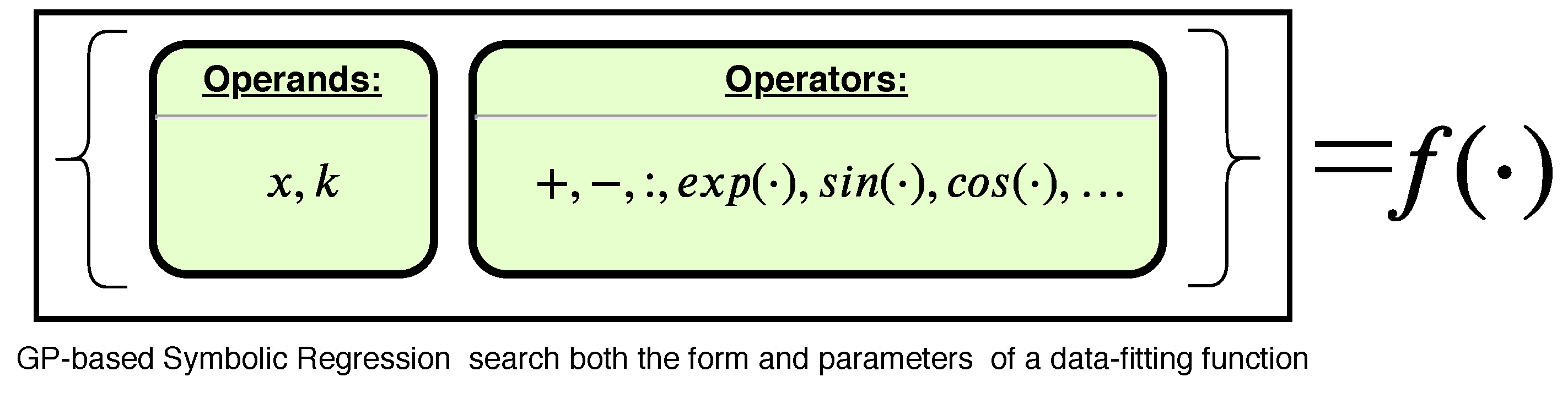
3.2.2. Method 2: Genetic Programming for Symbolic Regression

This kind of approach has been used to reveal the nonlinear relation between input signals and output available. This proposal can be used to discover not only the coefficients of the desired model but also the structure, i.e., how some kind of operations specified by the user could be used to process input signals to obtain the output reference. This reference is a reconstruction from the signal that comes from the balance under the machine during drying tests in the laboratory. The focus has been the development of this method applied to the problem at hand without a priori assumptions on the model (linear form, polynomial form, etc.) to discover suitable models for the purpose although hardly representable on a firmware version. Determination of an appropriate model structure is important to establish a benchmark and also to understand better the drying process itself observing which kind of inputs are combined and how.
Genetic programming (GP) is a type of evolutionary algorithm, a subset of machine learning related to supervised learning methods. It is a domain-independent method motivated by an analogy to biological evolution. GP creates successor hypotheses by repeatedly mutating and crossing over parts of the current best hypotheses, with the expectation to find a good solution in the evolution process. A Symbolic regression problem consists of finding the symbolic function that matches a given set of data as closely as possible (Figure 3). This method is usually used to discover governing equations from noisy measurement data [31]. In this work, it has been exploited to discover relations between the output (laundry moisture content) and signals already available online on the machine. A benchmarking of recent GP approaches to symbolic regression, in the context of state-of-the-art machine learning approaches, is available in [32].
In the GP approach, a population of computer programs is developed. The primary genetic operations are as follows.
  • Crossover: A child program is created from two selected parent programs by combining chosen parts randomly.
  • Mutation: A new child program is generated altering a randomly chosen part of a selected parent program.
Symbolic regression has been tested using a GP tool called “Genetic Programming Toolbox for the Identification of Physical Systems” (GPTIPS) [33] for use with MATLAB®. It employs a unique type of symbolic regression called multigene symbolic regression.
Solutions found by symbolic regression are compact, human-readable, and mathematically tractable, and this makes them potentially suitable for applications like the one at hand in this work.

3.2.3. Method 3: Polynomial Model for Drying Cycle Prediction

The approach discussed here deals a mathematical model developed to study the drying phenomenon of fabrics based on available data. Differently from the previous method, the structure of the model is fixed, but nonlinear, and determined after a preliminary offline analysis comparing some candidate forms provided by literature (models used to describe moisture transfer in food preservation and other areas different from fabric care).
Figure 4 shows an explanation of the proposed procedure in detail. The available dataset has been used offline to select the best model for the purpose, which was done by checking the performance of fitting (as summarized in Table 1 reported below), comparing each candidate model and the available output, which is the result of some elaborations from the signal of the weight evolution of laundry during drying cycle in laboratories. The best model between the candidates was chosen to consider some well-known indices used for goodness-of-fit analysis: Root-Mean-Square Error (RMSE) and coefficient of determination ( R 2 ). RMSE is represented in the next section; the coefficient of determination is the square of the correlation coefficient; a higher coefficient of determination is an indicator of better goodness of fit for the observations. Moreover, the number of parameters for each model was also taken into account, so as to avoid models that are too complex for firmware implementation.
The final trade-off (as shown in Table 1) was found in a 3rd degree polynomial model in time, ( t ) , and parameters a , b , c , d :
y ^ ( t ) = a + b t + c t 2 + d t 3
This is the structure that provides the best-fit performance on data (WD HP case study) and is proposed here as the model to explain the evolution of drying cycles of interest. After the fit analysis, the structure of the proposed model is fixed and the values of parameters for each observation as well (i.e., for each observation the fit analysis provides the values for a , b , c , and d, which are then used as the output reference for the linear regression step). Once the model and its true parameters are fixed, we need a procedure to estimate such parameters online using the available information from signals.
The chosen method follows a simple linear regression procedure, using some values computed from signals as inputs; these values will be called features and summarize the information provided by each available signal. These features were defined using expert knowledge and they are fixed. The handcrafted features used to estimate the parameters of the polynomial model are available after t * = 20 [min] from the beginning of the cycle, i.e., after 20 min from the start phase, an estimation of the laundry moisture content for the entire drying cycle is ready; examples of such features are quantities computed from temperature at the output of the drum and from the motor torque during drying. Details will be omitted here because of intellectual property rights.
Essential information exploited here is related to the (dry) weight of the laundry (dry laundry load estimation block in Figure 4—OFFLINE part), which is a value that is estimated online using the available information on the inertia of the laundry weight. Therefore, the information of the laundry weight quantity is used to train a linear model offline, which is different depending on the laundry weight: the structure of the model is always linear but the coefficients of the trained linear model vary depending on the laundry weight level.
Table 1 summarizes the results of fitting between moisture references and several models used for different drying applications (see also [14,20]); this study is represented as a “Fit Analysis” block in Figure 4—ONLINE part.
At the end of the offline part, the form of the model is available, together with the coefficients of linear models used to estimate the parameters of the polynomial structure; indeed, for each parameter, a linear model has been used exploiting the same set of defined features; therefore, in this case, four linear models are involved in this step. The online part is executed on the machine (WD-HP), and it deals with some simple passages: the first is the feature extraction process, which is performed computing the features defined in the offline part after the first phase of the cycle (20 min from the start). In this manner, we have time to collect useful information from signals. The second passage is the merging of the computed features with the coefficients determined in the offline part, and such a merging is composed of the linear models used to estimate the 3rd-degree polynomial parameters. The set of coefficients used by the firmware varies depending on the estimation provided by the laundry weight estimation procedure (dry laundry load estimation block in Figure 4—ONLINE part): once the estimation of the (dry) laundry load weight is available, it is used to select the correct set of coefficients of the linear models employed to determine the estimation of the moisture model parameters ( a * , b * , c * , d * ). Load estimation is done using linear models as well and particular features; details are not reported here. Therefore, for each load size, a set of linear models has been trained, for example,
a * = α 0 + α 1 h 1 + + α 7 h 7 b * = β 0 + β 1 h 1 + + β 7 h 7 c * = γ 0 + γ 1 h 1 + + γ 7 h 7 d * = δ 0 + δ 1 h 1 + + δ 7 h 7
where h i , i = 1 , , 7 are the features selected offline and α , β , γ , δ ; i = 0 , , 7 are linear regression coefficients.
Note that the computation of the drying rate, which is the derivative of the moisture content in time, can be useful to detect anomalous estimation of laundry, and this fact is exploited in Method 3 to modify the estimation in case. This situation is handled as a “control on shape” of the polynomial model (Figure 4). This simple control consists of a fixed decrease of the moisture for every predefined time interval (every minute). When the computed drying rate goes under a certain threshold (equal to 0 [ % / s ] ), the control starts and continues until the moisture target is reached ( 0 % in case of cotton).

4. Experimental Setting

The algorithm currently used on machines is not based on a measure or estimation of the most important output reference of a drying process, i.e., the laundry moisture content during a drying cycle. New proposals are focused on the estimation of this particular signal, which is difficult or costly to measure directly; for this reason, soft sensors (SSs) have been developed as new solutions for the problem at hand. Regarding the performance of a drying cycle algorithm, the main target is to improve the error in terms of final laundry moisture content, depending on the particular target (cotton, etc.) The moisture signal used as a reference to determine the performance of the procedures discussed in this work is not a direct measure from a dedicated physical sensor (there is no ad hoc sensor for washer-dryer machines of interest), therefore it is a result of some processing of the laundry weight signal, which is a measure available from laboratory (details about the elaborations from laundry weight evolution signal will be omitted here because of intellectual property rights). In particular, the available moisture reference is computed in percentage according to the following relation,
m o i s t u r e [ % ] = w e i g h t w c w c
where w e i g h t is the laundry weight signal obtained from a balance positioned under the machine during drying cycle after filtering and rescaling procedures, and w c is the conditioned weight, which is the weight of the dry laundry.
Several simulations have been performed using the same dataset with a different constraint on the size of input signals. In the next section, the main results, in terms of error distribution, are depicted. The estimated moisture value is provided for each t = 1 [s] by the model, and the estimation error is computed using the moisture reference that comes from the laundry weight signals available from data as said before. The represented error is the root-mean-square error (RMSE).
In Figure 5, the correlation matrix Γ I p × p , with I [ 0 , 1 ] and [ Γ ] i , j = | corr ( x i , x j ) | , of the available signals is depicted. In general, the correlation coefficient of two random variables is a measure of their linear dependence; the MATLAB function corrcoef was used here to compute such values. Every colored square in Figure 5 represents a degree of correlation between a couple of signals. The diagonal of Γ represents the correlations between the features and themselves, which are always equal to one. On the rest of the matrix, some areas tend to have higher correlation, because elaborations from the same original signals are in succession; for example, it correlated most couples in Figure 5, referring to the same rough temperatures.
As already mentioned, one focus for the techniques proposed here is the automatic EoC; therefore, from now on, all results will be reported in terms of RMSE considering the last part of the cycle (under 20 % of moisture). Therefore, RMSE will always be computed considering the estimated moisture ( y i ^ ( t ) ) and reference ( y ( t ) ) , considering the time interval for which the reference moisture is less than 20 % .
Details about the available dataset are reported here; Figure 6a,b shows the distribution of the available drying tests in terms of nominal weight (weight of dry laundry); in Figure 6b, the output reference is depicted (i.e., the laundry moisture evolution during drying obtained from the evolution of weight of the wet laundry during drying). The time series represented here were used as output reference to training models. It is easy to see that moisture references are very different comparing small and large loads. A number of 56 drying tests are available for the development and 30 signals acquired for each observation.
Regarding the methods introduced before about symbolic regression, some choices have been made to ensure the convergence of the optimization procedure implemented in the used tool and to reduce the overfitting risk due to models that are not suitable for test data.
In particular, the configuration setting is summarized and explained: ( i ) population size = 500; ( i i ) number of generations = 1000; ( i i i ) max number of genes ( G m a x ) = 5; ( i v ) max depth = 5; and ( v ) number of repeated simulations = 30. The first two points deal with the number of initial random models ( i ) and the number of allowed subsequent generations ( i i ) . The choice made for these two values is essential for the convergence of the optimization part of the algorithm performed by the GP procedure; there is no specific rule to choose them, but a rule of thumb is to follow a number of generations greater than population size, typically high values to avoid convergence problems. Clearly, the max number of genes (iii) Gmax is the number of trees or single models combined in the multigene approach; in this case, the value has been fixed to a low value equal to 5 to prevent overfitting problems when using models selected by symbolic regression on unknown test data.
For the same reason, the max depth ( i v ) allowed for each tree has been fixed to a low value to avoid too complex models. As explained before, GP is a stochastic approach because of the randomness of the initial population of models; therefore, a fixed number of repeated simulations, i.e., a loop for the entire symbolic regression code, has been imposed, ( v ) , to verify the robustness of GP to initial population. The number of iterations has been fixed to 30 in this case to avoid a huge computational effort; but, obviously, it should be set to a value as high as possible. In this case, values greater than 30 for the number of iterations turned out to be critical in terms of computational effort. The stopping criterion is related to the number of generations ( i i ) ; a high value was used here (1000) so as to be more confident about the convergence of the algorithm. The set of operations defined by the user and exploited by the tool to try models includes: sum, subtraction, multiplication, division, exponentials, logarithms, trigonometric functions, hyperbolic functions, absolute value, square, and cube functions; this set was chosen with the aim of satisfying a trade-off between flexibility and limits about the implementation burden (and taking into account the inspiration from physics—Section 3.1), but the authors emphasize that different other types of operations could be included.
The tool GPTIPS [33] used for this analysis helps the user to identify a model that looks promising for further investigation. In Figure 7, each model is plotted as a dot with ( 1 R 2 ) on the vertical axis and the complexity of the expression on the horizontal axis. As said before, the coefficient of determination R 2 is the square of the correlation coefficient, which is the ratio between the covariance of the two variables and the product of their standard deviations. The range is 0 to 1, so the target is to keep the difference ( 1 R 2 ) close to 0. The Pareto front models are highlighted in green (the model in the Pareto front are models that are not dominated by other models in the population in terms of model complexity and fitness). The final result for a single iteration is determined by the best trade-off between the model complexity and the fit error (red circled dot in Figure 7), which is automatically selected by the algorithm.
An entire moisture time series is selected randomly at each iteration to belong to a training or test set, and, for each case, the symbolic regression selects the best model according to the steps required by genetic programming. Performances in terms of RMSE for drying test i are computed: 1 n i t = 1 n i ( y i ( t ) y ^ i ( t ) ) , where n i is the number of samples for each observation and y ^ i is the estimation in the percentage of laundry moisture; error distributions are then visualized to evaluate the goodness of the provided models (see Section 5). The Estimation error is always computed considering the last part of the cycle—under 20 % of reconstructed moisture—because it is the part of interest in the application for the EoC.
Regarding Method 3, linear models, used to obtain the parameters a , b , c , and d for the model summarized in Equation (7), were trained using Regularized Linear Regression with the same sparse method used for Method 1 (LASSO) [3], which is exploited for its sparsity to select a set of statistically meaningful predictors (the features mentioned in Section 5.1). In this phase, 70 % of available observations for each load are used as the training set, while, the 30 % is used for test part in 100 Monte Carlo cross-validations. All results in this case also appear in terms of error distributions and visualized using box plots (Section 5.2).

5. Results

5.1. Method 1: Regularized Linear Regression

Several simulations have been performed using the same dataset with a different constraint on the size of input signals. In Figure 8a, our main results in terms of error distribution are depicted. The estimated moisture value is provided for each t = 1 [s] by the model, and the estimation error is computed using the moisture reference that comes from the laundry weight signals available from data, as said before. The represented error is the Root-Mean-Square Error (RMSE), and, in particular, from left to right, an increasing size of input signal has been used exploiting the sparsity of LASSO, imposing the input size as a degree of freedom in the code, e.g., LASSO1 stands for linear regression which uses lasso regularization with n s signals as inputs at most ( n s is a predefined value which is omitted here); thus, for each iteration, a number of signals (predictors) less than (or equal) to n s are selected by the algorithm and the error distribution of all the simulations performed are reported in the plot using box plot representation.
The median term of distribution in each box plot in Figure 8a is close to 3 % of error (RMSE), which means that in the last part of the drying cycle (the focus for the automatic EoC), the estimation of laundry moisture content shows a median term that is close to the threshold allowed for the target ( 3 % for Cotton). Each box plot is the distribution of 100 iterations of the Linear Regression using a different set of training and test observations (details about the size of each set are reported in the next paragraph). Figure 8b shows the normalized β values obtained for Method 1 from the CV iterations according to Equation (6) in terms of distribution. In particular, they refer to the first configuration depicted in Figure 8a (LASSO1), imposing the use of a maximum number of predictors equal to 5 for each iteration. This plot can visualize which predictors are the most useful for the purpose at hand and in this case, it appears that the main signals of temperatures and torque are the most statistically significant.
Some observations are reported here to sum up the main results achieved with the approach at hand:
  • The solution is simple and does not require particular effort for implementation: the use of a linear models makes the solution very easy because the signals used as inputs are already available online on WD HP machines and the information required is restricted to the values of β coefficients obtained with offline simulations.
  • With a small set of input signals, it is possible to achieve results with a RMSE between 3 % and 4 % of laundry moisture content, which is not sufficient to satisfy the target required by the industrial partner, but it is interesting result considering the simplicity of the method.
  • Using a bigger set of input signals leads to an improvement in terms of performance and it seems to be not possible to obtain moisture estimations with a RMSE under 2 % for the EoC using this kind of approach and the set of signals available.
In Figure 8c, the moisture target for one of the available observations together with the related estimation is depicted. Following this method, an update for the estimated value for laundry moisture is provided for each time sample ( [ s ] ) according to Equation (6). As the reader can easily see, the estimation is not smooth; this is due to the fact that signals used as predictors here are affected by noise. This method is the simplest one proposed here because the moisture is elaborated using signals already available as predictors combined in a linear model, but it is considered not suitable to solve other problems of interest, such as the Time-to-End (TTE) estimation problem, which consists of the determination of how much time is needed to detect the laundry moisture target. So, it is not possible to estimate the TTE a long time in advance during the drying cycle using the method at hand because the estimated moisture for a specific time sample changes according to the value assumed by each predictor at the time sample itself.

5.2. Method 2: Genetic Programming for Symbolic Regression

Figure 9a refers to Method 2 (Symbolic Regression with GP approach) and shows the results obtained so far, such as moisture error in percentage taking into account the final part of the drying cycle, which is the main part of interest for an automatic procedure for the EoC.
The entire set of available signals have been exploited here to collect the results. The obtained solutions are visualized in the distribution in Figure 9a, but each iteration could give a different result in terms of the structure of the selected model, e.g., one solution is the following,
y ^ = k 0 + k 1 x 2 3 + k 2 x 7 x 2 + k 3 x 3 + k 4 x 7 + k 5 x 8 + k 6 x 16 + k 7 x 21 + k 8 x 23 + k 9 x 26 + k 10 x 27
where k i , i = 1 , , 10 are found coefficients and x i are signals.
The solution selected at the next iteration can show different powers of the involved input signals, but the goal here is the discovery of the most useful models for the purpose, i.e., which structures have been selected more frequently in all iterations (if any). It turns out that the most selected structures are the ones that involve main signals of temperatures and motor torque (or signals that are the elaboration of those); this confirms that these are also the meaningful signals for the goal. Furthermore, polynomial terms are selected mostly (instead of exponentials or trigonometric functions). The results from Methods 1 and 2 suggest that nonlinear combinations of input signals do not improve the performance in general and is supposed to be due to the problem of overfitting, which is still present even though much reduced.

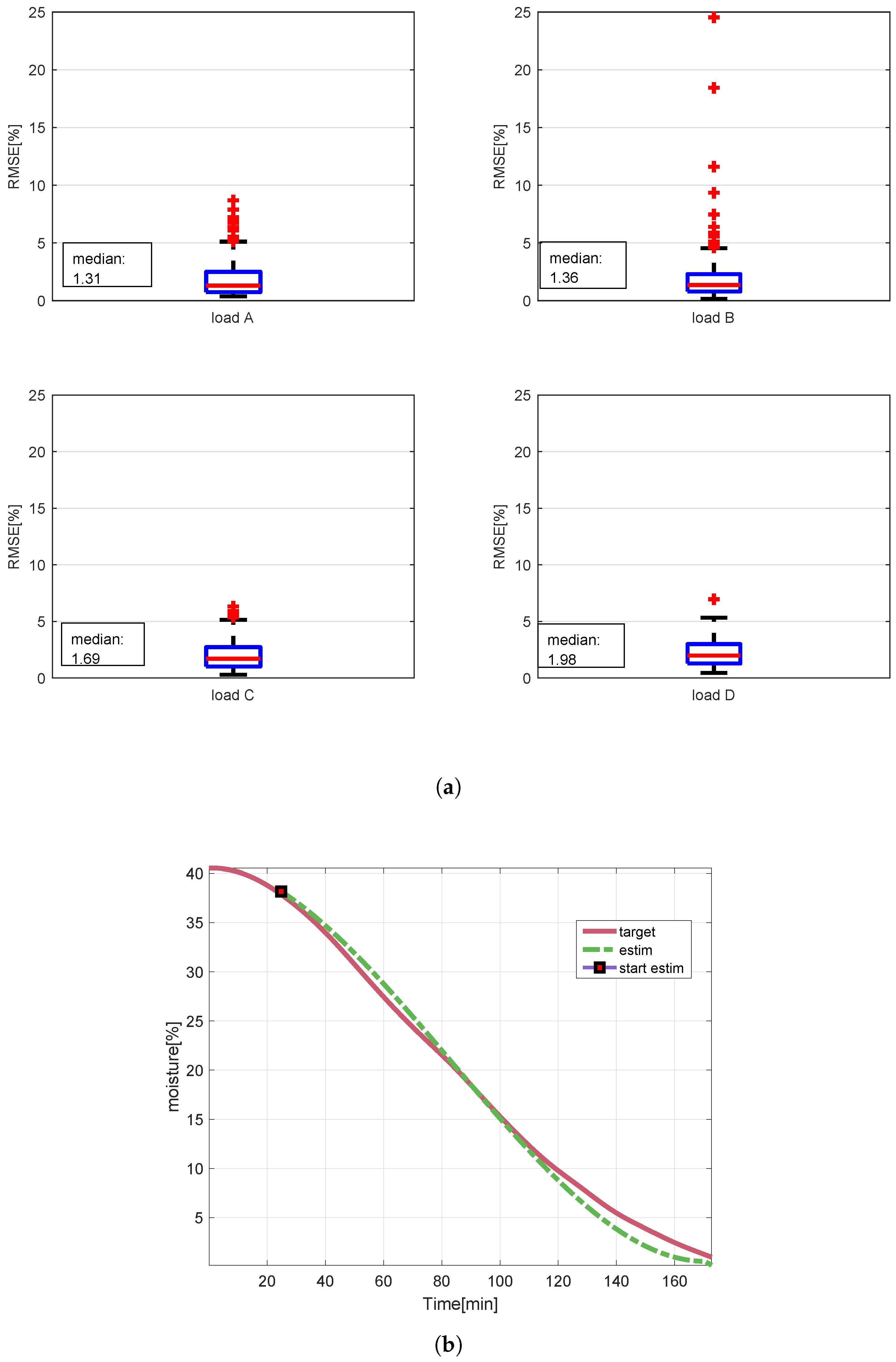
5.3. Method 3: Polynomial Model for Drying Cycle Prediction

In Figure 10a, the results, in terms of error distribution, are represented. In this case, the variability of the error is high, and it is due to the variability of the estimation of parameters of the polynomial model; nevertheless, the focus now is on the reduction of this variability.
In particular, Figure 10a shows the results for each laundry load amount while considering the fact that the algorithm exploits a load estimation phase (as represented in Figure 4).
As depicted in Figure 10a, the median term in each distribution (in percentage of moisture) is very low and always under the limit of 3 % , which is considered the threshold for an acceptable performance for the end-of-the cycle in cotton laundry typology, which is the case study at hand, but the current problem which is still present is the error variability as explained before. Figure 10b also shows an example of an estimation of the laundry moisture content during drying, which was made using the polynomial model compared with the reference for the specific observation. Note that the use of this approach (polynomial shape of the moisture estimation) is preferred as a solution because of its smoothness. In fact, in this case, inputs are features computed from signals and used to estimate parameters of the fixed model. Once the estimation of parameters of the model is ready, the result is a 3rd degree polynomial in time, which is smooth in contrast to results obtained with other approaches.
Table 2 summarizes the comparison between (data-driven) methods proposed in this work as procedures to estimate the laundry moisture evolution on household drying machines during drying process. The method named “Current algorithm” refers to the current procedure implemented online on machines, and it is mentioned here to make clear the features of each proposed procedure and the contribution for each item of interest (details about it will be omitted here because of intellectual property rights). Items summarized here are the main requests made by the industrial partner with the goal of selecting a new algorithm for the control of the drying cycles on machines. The main focus is clearly on performance but also on the complexity and calibration effort to avoid some time-consuming procedures involved in the use of the current algorithm.
Regarding the criteria mentioned in Table 2, EoC and TTE feasibility refer to the possibility of carrying out the automatic end-of-the-cycle and time-to-end using one method or another. In particular, the interest is the chance to compute at the beginning of the cycle how much time is needed to reach the estimated moisture target; in this respect, methods that provide an estimation of moisture, which depends on the current values of the input signals (like Methods 1 and 2), are not suitable for a direct computation of the TTE. In these cases, the automatic EoC is possible because it is determined when the (estimated) moisture target is reached; on the other hand, the TTE task requires in these cases an additional dedicated algorithm. Therefore, it cannot use the provided estimation directly to determine the TTE. In this perspective, Method 3 is quite different because it allows an estimation of the laundry moisture evolution as a time series, using features computed at the beginning of the drying cycle. It permits an evaluation of the TTE once the model is available (after 20 min from the start phase). In fact, once the estimation of the parameters of the poly3 is available (Equation (7)), it is possible to determine the time needed to reach the moisture target y .
Figure 8a and Figure 9a show that Methods 1 and 2, in terms of performance, are not suitable for the predefined target (error distribution under 3 % ), although otherwise acceptable in terms of variance. As seen in Figure 10a, there still exists a problem related to the variance of estimation error in the use of Method 3, especially for load B. Some new constrains on estimated values of parameters of the cubic model (7) have been imposed in order to reduce the error variance, taking into account the fact that drying tests in laboratory are time-consuming and no more data are available for this work now. The use of a richer dataset could be a next-step of this project; here, the goal was to develop SSs using already available tests made for different projects, avoiding dedicated Design of Experiments (DOE) tests. The last two columns in Table 2 show a comparison in terms of calibration and implementation effort. Regarding the former, the current algorithm in production suffers from a time-consuming calibration phase because operators must fix some thresholds on the EoC signal and these thresholds have to be managed on firmware. In the latter case, Method 2 suffers from an additional complexity level because the model selected by Symbolic Regression could include some nonlinear terms which are difficult to write on firmware, e.g., combinations of exponential, trigonometric functions etc. The other methods are simpler to represent online because signals are combined linearly (Method 1) or because the model is a time series with few parameters (Method 3).

6. Conclusions

The present work aims at developing SSs for fabric care major appliances, with the purpose of improving the performance of the drying algorithm on the market and simplifying the calibration phases of them. More precisely, this work deals with the development of Soft Sensors to estimate laundry moisture content in household heat-pump washer–dryers during drying, to improve drying performance and user experience. This paper focuses on
  • the use of different approaches to obtain the estimation of laundry moisture content during drying cycles in the domestic washer–dryers, and
  • the determination of the best model to provide the estimation of laundry moisture content as a time series obtaining a smooth curve to predict the end-of-the-cycle automatically.
Regarding the first point, experimental data were used to train models with available signals as predictors and laundry moisture content samples as the output in a supervised manner. Models were chosen by imposing a linear structure (Method 1) or using the symbolic regression approach (Method 2), which exploits genetic programming to construct nonlinear combinations from data and provides coefficients for such a model. Unlike other methods, Method 3 exploits features computed in the first part of the cycle to predict the parameters of a polynomial model in time whose structure is determined a priori.
The operating difference between the proposed methods relies on the nature of the model: in linear or symbolic regression predictors are signals, and they are combined in different (nonlinear) ways; while using the 3rd-degree polynomial model (Equation (7)—Method 3), the prediction is a time series and the difficulty is on the online estimation of the parameters of such a model.
The Main results of the work described in this paper can be summarized as below.
  • The best nonlinear models selected by symbolic regression (Method 2) always involve main signals of temperatures and motor torque (or signals that are an elaboration of those), which confirm the result obtained using sparse regularization and linear regression (Method 1), where the structure of the model is fixed and always linear. These types of signals are, therefore, the most useful for the purpose. The models provided by methods 1 an 2 use available signals as predictors, which affect the estimation with their noise.
  • The best model for the description of laundry moisture content as a time series is the 3rd-degree polynomial model (7) (Method 3), and it comes from a comparison between several models from Table 1; this is the best model to describe laundry moisture content during the drying cycles based on available real data.
Deep learning (DL) frameworks [34] were not exploited in this work, mainly because of the lack of a suitable number of complete drying cycles, which can lead to overfitting behaviors. Another reason is the fact that, for the purpose at hand, the interpretability of the developed models is mandatory; therefore, the use of DL architectures was considered unsuitable even though possible [1].
In addition, two strengths of this work need to be underlined: (i) The novelty of the work: to the best of our knowledge, there are no similar cases in the literature concerning the online estimation of parameters of a moisture transfer model through porous media like laundry. (ii) An effective “soft” approach: no impact on hardware and no dedicated Design of Experiments (DOE) were required.

7. Patents

An international patent application has been filed recently for Method 3, discussed above (Patent P-62396/WO1).

Author Contributions

Conceptualization, G.Z., G.A.S., T.G., G.R.-M., L.d.S.C., and M.R.; methodology, G.A.S., A.B., T.G., G.R.-M., and L.d.S.C.; software, G.Z. and N.F.; validation, T.G., G.A.S., and G.R.-M.; formal analysis, G.Z. and G.A.S.; investigation, G.Z. and G.A.S.; resources, T.G.; data curation, T.G., G.Z., and N.F.; writing—original draft preparation, G.Z.; writing—review and editing, G.A.S., M.R., and A.B.; visualization, G.Z. and N.F.; supervision, G.A.S., A.B. M.R., G.R.-M., and L.d.S.C.; project administration, A.B. and F.A.; funding acquisition, F.A. and A.B.

Funding

This research was funded by Electrolux Italia S.p.A.

Acknowledgments

Electrolux Italia S.p.A. is gratefully acknowledged for the support and real data provided.

Conflicts of Interest

The authors declare no conflicts of interest.

Abbreviations

The following abbreviations are used in this manuscript:
CVCross-Validation
DLDeep Learning
DOEDesign of Experiments
EoCEnd-of-the-Cycle
GPGenetic Programming
LASSOLeast Absolute Shrinkage and Selection Operator
RMSERoot-Mean-Square Error
RRRidge Regression
RSSResidual Sum of Squares
SSSoft-Sensors
TTETime-to-End
WD-HPWasher Dryer–Heat Pump (technology)

References

  1. Shang, C.; Yang, F.; Huang, D.; Lyu, W. Data-driven soft sensor development based on deep learning technique. J. Process Control 2014, 24, 223–233. [Google Scholar] [CrossRef]
  2. Susto, G.A.; Johnston, A.B.; O’Hara, P.G.; McLoone, S. Virtual metrology enabled early stage prediction for enhanced control of multi-stage fabrication processes. In Proceedings of the IEEE International Conference on Automation Science and Engineering (CASE), Madison, WI, USA, 17–20 August 2013; pp. 201–206. [Google Scholar]
  3. Trevor, H.; Robert, T.; JH, F. The Elements of Statistical Learning: Data Mining, Inference, and Prediction; Springer: Berlin/Heidelberg, Germany, 2009. [Google Scholar]
  4. Kadlec, P.; Gabrys, B.; Strandt, S. Data-driven soft sensors in the process industry. Comput. Chem. Eng. 2009, 33, 795–814. [Google Scholar] [CrossRef]
  5. Soares, S.G. Ensemble Learning Methodologies for Soft Sensor Development in Industrial Processes. Ph.D. Thesis, Coimbra, Portugal, 2015. [Google Scholar]
  6. Susto, G.A.; Zambonin, G.; Altinier, F.; Pesavento, E.; Beghi, A. A soft sensing approach for clothes load estimation in consumer washing machines. In Proceedings of the IEEE Conference on Control Technology and Applications (CCTA), Copenhagen, Denmark, 21–24 August 2018; pp. 1252–1257. [Google Scholar]
  7. Susto, G.A.; Maggipinto, M.; Zannon, G.; Altinier, F.; Pesavento, E.; Beghi, A. Machine Learning-based laundry weight estimation for vertical axis washing machines. In Proceedings of the IEEE European Control Conference (ECC), Limassol, Cyprus, 12–15 June 2018; pp. 3179–3184. [Google Scholar]
  8. Zambonin, G.; Altinier, F.; Corso, L.; Sessolo, M.; Beghi, A.; Susto, G.A. Soft sensors for estimating laundry weight in household heat pump tumble dryers. In Proceedings of the IEEE 14th International Conference on Automation Science and Engineering (CASE), Munich, Germany, 20–24 August 2018; pp. 774–779. [Google Scholar]
  9. Susto, G.A.; Vettore, L.; Zambonin, G.; Altinier, F.; Beninato, D.; Girotto, T.; Rampazzo, M.; Beghi, A. A machine learning-based soft sensor for laundry load fabric typology estimation in household washer–dryers. In Proceedings of the IFAC Conference on Intelligent Control and Automation Science (ICONS), Belfast, Northern Ireland, 21–23 August 2019. [Google Scholar]
  10. Schölkopf, B.; Smola, A.J. Learning with Kernels: Support Vector Machines, Regularization, Optimization, and Beyond; MIT Press: Cambridge, MA, USA, 2002. [Google Scholar]
  11. Scheidegger, A.E. The physics of flow through porous media. Soil Sci. 1958, 86, 355. [Google Scholar] [CrossRef]
  12. Luikov, A.V. Heat and mass transfer in capillary-porous bodies. In Advances in Heat Transfer; Elsevier: Amsterdam, The Netherlands, 1964; Volume 1, pp. 123–184. [Google Scholar]
  13. Doymaz, İ. Effect of dipping treatment on air drying of plums. J. Food Eng. 2004, 64, 465–470. [Google Scholar] [CrossRef]
  14. Kucuk, H.; Midilli, A.; Kilic, A.; Dincer, I. A review on thin-layer drying-curve equations. Dry. Technol. 2014, 32, 757–773. [Google Scholar] [CrossRef]
  15. Younis, M.; Abdelkarim, D.; El-Abdein, A.Z. Kinetics and mathematical modeling of infrared thin-layer drying of garlic slices. Saudi J. Biol. Sci. 2018, 25, 332–338. [Google Scholar] [CrossRef] [PubMed]
  16. Dincer, I. Energy and environmental impacts: Present and future perspectives. Energy Sources 1998, 20, 427–453. [Google Scholar] [CrossRef]
  17. Ketelaars, A.; Pel, L.; Coumans, W.; Kerkhof, P. Drying kinetics: A comparison of diffusion coefficients from moisture concentration profiles and drying curves. Chem. Eng. Sci. 1995, 50, 1187–1191. [Google Scholar] [CrossRef] [Green Version]
  18. Sahin, A.; Dincer, I.; Yilbas, B.; Hussain, M. Determination of drying times for regular multi-dimensional objects. Int. J. Heat Mass Transf. 2002, 45, 1757–1766. [Google Scholar] [CrossRef]
  19. Prasertsan, S.; Saen-Saby, P. Heat pump drying of agricultural materials. Dry. Technol. 1998, 16, 235–250. [Google Scholar] [CrossRef]
  20. Haghi, A.; Ghanadzadeh, H. A study of thermal drying process. Indian J. Chem. Technol. 2005, 12, 654–663. [Google Scholar]
  21. Sander, A.; Kardum, J.P. Experimental validation of thin-layer drying models. Chem. Eng. Technol. Ind. Chem.-Plant Equip.-Process Eng.-Biotechnol. 2009, 32, 590–599. [Google Scholar] [CrossRef]
  22. Hamdaoui, M.; Baffoun, A.; Chaaben, K.B.; Hamdaoui, F. Experimental study and mathematical model to follow the drying phenomenon of knitted textile fabric. J. Eng. Fibers Fabr. 2013, 8. [Google Scholar] [CrossRef]
  23. Crank, J. The Mathematics of Diffusion; Oxford University Press: Oxford, UK, 1979. [Google Scholar]
  24. Dincer, I.; Zamfirescu, C. Drying Phenomena: Theory and Applications; John Wiley & Sons: Hoboken, NJ, USA, 2016. [Google Scholar]
  25. Pan, N.; Gibson, P. Thermal and Moisture Transport in Fibrous Materials; Woodhead Publishing: Sawston, UK, 2006. [Google Scholar]
  26. Van Oudenaarden, A. Cell Systems Biology Lecture; Course: Systems Biology, Modeling Biological Networks; Technical Report; MIT: Cambridge, MA, USA, 2009. [Google Scholar]
  27. Luikov, A.V. Analytical Heat Diffusion Theory; Elsevier: Amsterdam, The Netherlands, 2012. [Google Scholar]
  28. Berger, J.; Gasparin, S.; Dutykh, D.; Mendes, N. Accurate numerical simulation of moisture front in porous material. Build. Environ. 2017, 118, 211–224. [Google Scholar] [CrossRef] [Green Version]
  29. Gasparin, S.; Berger, J.; Dutykh, D.; Mendes, N. Advanced reduced-order models for moisture diffusion in porous media. Transp. Porous Media 2018, 124, 965–994. [Google Scholar] [CrossRef]
  30. Azeem, M.; Boughattas, A.; Wiener, J.; Havelka, A. Mechanism of liquid water transport in fabrics; a review. Fibres Text. Vlákna Text. 2017, 4, 58–62. [Google Scholar]
  31. Sharma, S.; Tambe, S.S. Soft-sensor development for biochemical systems using genetic programming. Biochem. Eng. J. 2014, 85, 89–100. [Google Scholar] [CrossRef]
  32. Orzechowski, P.; La Cava, W.; Moore, J.H. Where are we now? A large benchmark study of recent symbolic regression methods. In Proceedings of the Genetic and Evolutionary Computation Conference, Kyoto, Japan, 15–19 July 2018; ACM: New York, NY, USA, 2018; pp. 1183–1190. [Google Scholar]
  33. Searson, D.P. GPTIPS 2: An open-source software platform for symbolic data mining. In Handbook of Genetic Programming Applications; Springer: Berlin/Heidelberg, Germany, 2015; pp. 551–573. [Google Scholar]
  34. Goodfellow, I.; Bengio, Y.; Courville, A. Deep Learning; The MIT Press: Cambridge, MA, USA, 2016. [Google Scholar]
Figure 1. Particles randomly move through the porous medium according to a diffusion process; the arrows (vectors) represent also the flux of water particles.
Energies 12 03843 g001
Figure 2. A Visual explanation of the algorithm proposed as Method 1. For each time sample, an estimation value is available (e.g., dot depicted in each plot).
Energies 12 03843 g002
Figure 3. Representation of genetic programming (GP)-based symbolic regression; y = laundry moisture content during the drying cycle, x = independent variables (signals available), and k = parameters.
Energies 12 03843 g003
Figure 4. A Visual explanation of the algorithm proposed in Method 3.
Energies 12 03843 g004
Figure 5. Visualization of the correlation matrix (absolute values of correlation are reported): each row and column stands for an available signal.
Energies 12 03843 g005
Figure 6. Data visualization by (dry) laundry load weight: (a) Laundry load weight distribution in the data, 4 classes in kg, and (b) laundry moisture reference.
Energies 12 03843 g006
Figure 7. Multigene regression model population. Diamonds represent the Pareto front of models visualizing the model performance ( 1 R 2 ) and complexity. Non-Pareto models are represented with dots. The best model (in terms of R 2 ) on the data used for training in the population is represented with a square.
Energies 12 03843 g007
Figure 8. Examples of results using Method 1: (a) Performance in terms of RMSE distribution (in % moisture content) using regularized linear models; the size of input signals increases from left to right. (b) Variable selection made by the LASSO imposing the use of few predictors (LASSO1) for each iteration. The term Constant on x-axis is the intercept of the linear models for which coefficients are represented here. (c) Example of laundry moisture content estimation using all predictors (RR); on y-axis, the moisture content in percentage.
Energies 12 03843 g008
Figure 9. Examples of results using Method 2: (a) Performance in terms of RMSE distribution (in % moisture content) using symbolic regression with a GP approach with all input signals available; the increasing size of the input signals from left to right. (b) Example of laundry moisture content estimation using all predictors available; on the y-axis the moisture content in percentage.
Energies 12 03843 g009
Figure 10. Examples of results using Method 3: (a) Current performance in terms of RMSE distribution (in % moisture content) using Method 3. The results divided by laundry nominal load are listed with increasing size of input signals from left to right. (b) An example of laundry moisture content estimation using the 3rd-degree polynomial model in time, on y-axis the moisture content in percentage (the square represents the time in which the estimation is provided during drying cycle).
Energies 12 03843 g010
Table 1. Drying models fitted to experimental data; t = time and y = moisture.
ModelExpressionRMSE [%] R 2 Index#Params
Lewis y = e a t 9.0690.7812
Henderson & Pabis y = a e b t 1.1470.9963
quadratic y = a + b t + c t 2 1.0510.9973
poly3 y = a + b t + c t 2 + d t 3 0.3990.9994
rational y = a + b t 1 + c t + d t 2 6.5640.8974
gaussian y = a e ( t b ) 2 2 c 2 0.4170.9994
sigmoid y = a + b 1 ( 1 + c e t ) 0.4960.9993
two exp y = a e b t + c e d t + e 0.7460.9985
mixed y = a e b t + c t 2 + d t + e 0.4530.9995
Table 2. Comparison between the proposed methods; * = the target for performance refers to the EoC estimation error, i.e., the error between the moisture reference and the estimate. The target formalized is to remain under a certain value of the error quantified using the RMSE metric defined before.
MethodsEoC FeasibilityTTE FeasibilityPerformance Target *Low Error VarianceAlgorithm CalibrationImplementation Facility
Method 1
Method 2
Method 3
Current algorithm

