Article

A State of Health Estimation Framework for Lithium-Ion Batteries Using Transfer Components Analysis

1
College of Information Engineering, Capital Normal University, Beijing 100048, China
2
Beijing Key Laboratory of Electronic System Reliability Technology, Capital Normal University, Beijing 100048, China
*
Author to whom correspondence should be addressed.
Energies 2019, 12(13), 2524; https://doi.org/10.3390/en12132524
Submission received: 16 May 2019 / Revised: 20 June 2019 / Accepted: 28 June 2019 / Published: 30 June 2019
(This article belongs to the Section F: Electrical Engineering)

Abstract

:
As different types of lithium batteries are increasingly employed in various devices, it is crucial to predict the state of health (SOH) of lithium batteries. There are plenty of methods for SOH estimation of a lithium-ion battery. However, existing technologies often have computational complexity. Furthermore, it is difficult to use least the previous 30% of data of the battery degradation process to predict the SOH variation of the entire degradation process. To address this problem, in this paper, the SOH of the target battery is estimated based on the transfer of different battery data sets. Firstly, according to importance sampling (IS), valid features are extracted from cycles of charging voltage in both the source and target battery. Secondly, transfer component analysis (TCA) is used to map the source data set to the target data set. Moreover, an extreme learning machine (ELM) algorithm is employed to train a single hidden layer feed forward neural network (SLFN) for its fast training speed and facile to set up. Finally, validation experiments and the comparisons on the results are conducted. The results showed that the proposed framework has a good capability of predicting the SOH of lithium batteries.

1. Introduction

In recent decades, lithium batteries, as power units of numerous mobile terminals, have been becoming more and more widely used in various electronic devices, especially for electric vehicles (EV) and energy systems [1]. However, the capacity of lithium-ion batteries will drop off with charge and discharge operations. In order to ensure the stability of devices, technologies for SOH are often adopted to estimate the current degradation degree of the lithium-ion battery [1,2,3,4]. Therefore, predicting the SOH of a battery is attached with essential significance. There are many kinds of valid SOH estimation methods for a lithium-ion battery [2,3,4]. However, in practical applications, it is still challenging to predict the long-term SOH of the battery when the battery has only been used for 20% to 50% of its life.
In this paper, the SOH of the lithium-ion battery refers to the ratio of battery discharge capacity to new battery rated capacity under certain conditions, which is shown as follows:
S O H = C i C 0 × 100 % .
In the past decades, extensive research has been conducted into the SOH of batteries. Battery SOH prediction can be divided into two categories: adaptive methods and data-driven methods [2,3,4]. Adaptive prognostic approaches, such as Kalman filter (KF) and particle filter (PF), intend to make an optimal estimate of the state of the system in terms of minimum variance. Zheng et al. [5] integrates UKF (unscented Kalman filter) and relevance vector regression (RVR) to make short-term predictions of the capacity fade trend of a lithium battery. They optimized the output of RVR using the UKF algorithm based on the physical degradation model. UKF is an algorithm based on the combination of unscented transformation and KF. This algorithm mainly uses the KF idea, but when solving the predicted value and the measured value at the subsequent time of the target, it is necessary to apply the sampling point to calculate. Rémy Mingant et al. present the quasi-electrochemical impedance spectrum (QEIS) for battery SOH prognostication [6]. Zhang et al. used UKF to predict the state of charge (SOC) and SOH of the battery by internal resistance [7]. However, the measurement of internal resistance requires specialized instruments. Fang et al. proposed the double extended Kalman filter (DEKF), an improved extended Kalman filter (EKF) algorithm [8]. This algorithm finds the function between internal resistance and capacity by establishing an equivalent circuit model to track the change in internal resistance of the battery. Further, the forgetting factor recursive least-squares method is used for online parameters identification. The research results of adaptive approaches are abundant. But, the common shortcoming of these methods is the complexity of mathematical calculations due to numerous parameters [2]. In practice, the different ways of operation and noise will lead to misalignment of the entire intricate model.
Support vector machine (SVM) [9] and artificial neural network (ANN) have been rising as the most essential data-driven methods. SVM solves the linear separability of samples by mapping samples to high-dimensional space, and ANN is a multi-layered computing model in which nodes between layers are connected to each other. ANN has the ability to handle nonlinear systems; but, data-driven methods also require high calculations. Hannan et al. used a backtracking search algorithm (BSA) to optimize back propagation neural network (BPNN) to predict battery SOC and SOH changes under various operating conditions [10]; and the prediction accuracy has improved. Compared with particle swarm optimization and genetic algorithm, BSA is a simpler and more efficient optimization algorithm [11]. Kim et al. proposed using a multi-layer perceptron, which is a primary ANN model for predicting SOH [12]. This article uses some discrete segments of the entire battery life span to train the model, and also has high accuracy in the untrained portion. However, these discrete battery data and SOH are also obtained under conditions of known complete life span, which makes the meaning of prediction relatively weak. He et al. built a dynamic Bayesian network in combination with the SOC and terminal voltage of the battery. Additionally, a forward propagation algorithm is used to realize the online prediction of SOH [13]. Zhang et al. introduced long short-term memory (LSTM) to learn the long-term dependencies of every cycle of batteries [14]. Liu et al. proposed a framework based on adaptive recurrent neural network (ARNN) to directly predict the SOH of lithium batteries [15]. ARNN is based on a triple layer feed-forward neural network (FFNN). The output of the hidden layer is delayed and passed to the hidden layer via recurrent feedback. However, the feature data used in this model is the internal impedance data of the battery, which is difficult to obtain. Wu et al. [16] focused on the feature selection problem of machine learning methods. Importance sampling (IS) is used to sample differential data of different cyclic charging voltage and valid results achieved.
There are growing types of lithium batteries used in different electronic devices. Present NN crafts require degradation data collected in the same environment and from the same type of battery. A traditional NN regression learner cannot be used for distinct battery SOH prediction, which promotes the employment of the domain adaptation method. Therefore, it is difficult and meaningful to use least the previous 30% of data of the battery degradation process to predict the SOH variation of the entire degradation process. In this paper, an online framework based on the domain adaptation (DA) approach is proposed to solve the predicament of SOH prediction of a different new type of lithium-ion battery. By mapping an already known lithium-ion battery data set to a new feature space, a similar complete data set of the new type of battery can be obtained. Therefore, a further regression learner is easy to obtain.
In the last few decades, many improved algorithms based on gradient descent (GD) have been developed. BPNN (back propagation neural network) with improved efficient training algorithm cannot jump out of the limitations of BPNN. This model still takes a long time of iterative training. Thus, ELM is introduced instead of GD to train an FFNN because of its fast training speed and low calculation cost.
Transfer learning has been an emerging learning method in recent years. In the traditional machine learning method, the training data and the test data are required to be identically distributed, otherwise the prediction result may shift [17,18]. The rise of migration learning is precisely to solve this drift problem. In transfer learning, there are two types of data with similar distribution. One type of knowledge that contains known knowledge is called the source domain, which is the object to be transferred, and the other is the data that are unknown, but similar to the source domain knowledge. This is called the target domain and is the target of transfer. The goal of transfer learning is that the source domain gains some knowledge in the solution task to improve the target task.
The following of this paper is structured as follows. In Section 2, a domain adaptation algorithm and a triple layer FFNN training method are introduced, after which the composition of the framework called transfer component analysis (TCA)-extreme learning machine (ELM) is presented. The experimental data set is introduced in Section 3. Experimental design ideas, experimental results, and corresponding analysis are introduced in Section 4. Conclusion are conducted in Section 5.

2. Applied Approaches

This section is used to introduce the approaches that are applied to exploit the knowledge of the complete degradation data of a source battery for the prediction of target battery SOH; it is composed of two parts. The first part introduces usage of domain adaptation method. The second part introduces the neural network training algorithm used in this paper.

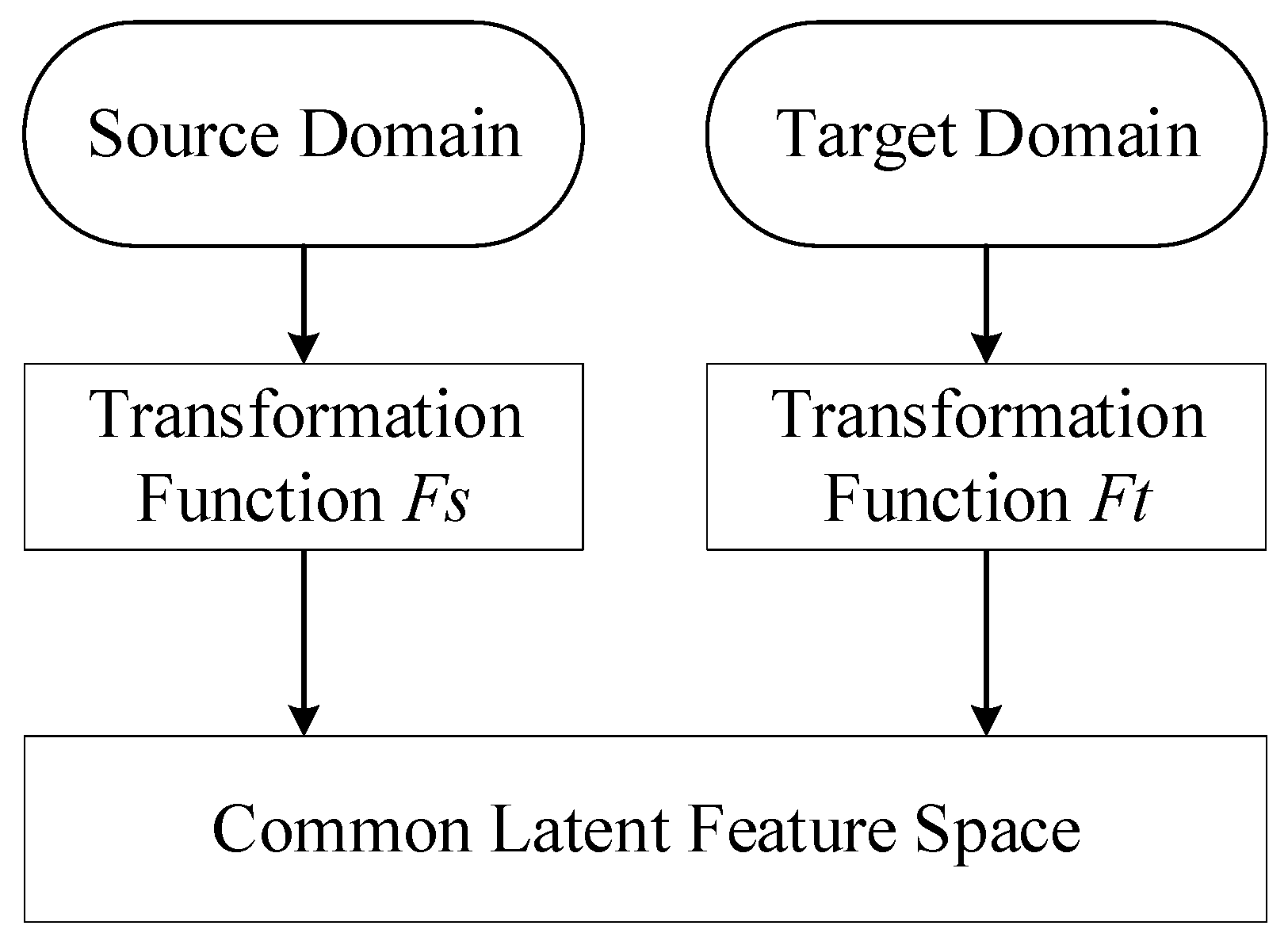
2.1. Domain Adaptation

Pan et al. [19] proposed TCA, which is a symmetric feature-based DA approach that aims to reduce the difference of feature data between the source domain and target domain [17,18].
These two domains have the same feature space and similar, but distinct marginal distributions. As is shown in Figure 1, the principle of TCA is to map the feature data of two differently distributed domains onto the general latent feature space based on reproducing kernel Hilbert space (RKHS). The difference between the two domains is measured by maximum mean discrepancy (MMD), which is defined as follows:
d i s t = 1 m 1 i = 1 m 1 f ( x s i ) 1 m 2 j = 1 m 2 f ( x t j ) H ,
where H represents RKHS, x s i indicates the ith sample of source domain, x t j indicates the jth sample of target domain, and f (   ) indicates the mapping function of the two domains mapping feature data from present feature space to the latent shared feature space. The main focal point of TCA is how to find f (   ) quickly and efficiently. There could be numerous f (   ) . Therefore, by introducing the kernel method, Pan amended Equation (2) into the following:
d i s t = t r ( K L ) ,
K = [ K s , s K s , t K t , s K t , t ] ,
where K s , s is the kernel matrix of the source domain data obtained through the mapping of kernel function k ( , ) . K s , t , K t , s , and K t , t can be obtained by analogy of K s , s ; and
L = { 1 m 1 2 x , y s r c 1 m 2 2 x , y t a r 1 m 1 m 2 o t h e r w i s e .
It has changed into a semi-definite programming (SDP) problem after this transformation. As the SDP formula is time-consuming in calculation, Pan introduced a dimension reduction method to construct the desired result [19]. Scholkpf et al. [20] proposed a method for reducing the dimensionality of the kernel matrix for nonlinear principle components analysis (PCA). The kernel matrix in Equation (4) can be implemented as
K = ( K K 1 / 2 ) ( K 1 / 2 K ) .
The dimension of the dimensionality reduction space is d m 1 + m 2 . In that way, a ( m 1 + m 2 ) × d matrix W ˜ , which is used to map the corresponding source and target domain feature vectors to low-dimensional space, can be constructed. Also, the kernel matrix can be rewritten into the following:
K ˜ = ( K K 1 / 2 W ˜ ) ( W ˜ K 1 / 2 K ) = K W W T K .
In particular, W = K 1 / 2 W ˜ is a lower-dimensional solution than K . Equation (3) can be mathematically expressed as follows:
d i s t = t r ( ( K W W T K ) L ) .
In order to optimize Equation (8) and reduce the complexity of the matrix, the regularization term t r ( W T W ) is added to Equation (8) by Pan [19]. At this point, TCA can be summarized as follows:
min W t r ( ( K W W T K ) L ) + μ t r ( W T W ) s . t . W T K H K W = I ,
where I is a ( m 1 + m 2 ) × ( m 1 + m 2 ) unit matrix. H = I 1 / ( m 1 + m 2 ) A is a center matrix and A is an ( m 1 + m 2 ) ( m 1 + m 2 ) all-one matrix, respectively. To maintain the diverse of the data, additional constraint W T K H K W = I is used to limit the divergence of data.

2.2. Training Algorithm of Neural Network

ELM, which is an emerging neural network (NN) training algorithm for single hidden layer feed forward neural network (SLFN), was proposed by Huang et al. [21,22]. It differs from the traditional training algorithm of SLFN; because there is no iteration in ELM trained NN, it achieved a fast training speed.
In this paper, a distinct sample is denoted as ( x i , y i ) , where x i = [ x i 1 , , x i p , , x i n ] R n and y i is the corresponding output. The structure of ELM is shown in Figure 2.
The input layer has n input neurons, corresponding to the n-dimensional features of a sample. The hidden layer has L hidden neurons, and L N . N denotes the number of samples. w p j denotes the weight between the pth input layer neurons and the jth hidden layer neurons and b j denotes jth bias of hidden layer neurons. β j denotes jth weight between hidden layer neurons and output layer neurons. This model can be summarized as follows:
H β = Y ,
where
H = [ g ( p = 1 n x i p w p 1 + b 1 ) g ( p = 1 n x i p w p L + b L ) g ( p = 1 n x i p w p 1 + b 1 ) g ( p = 1 n x i p w p L + b L ) ] N × L   , β = [ β 1 β L ] L × 1 ,   and   Y = [ y 1 y N ] N × 1 .
Training an SLFN is equivalent to finding a least-squares solution β ˜ = H T of the problem. Where H is the pseudo-moores inverse of the matrix H. The resulting β ˜ is the global optimal solution.

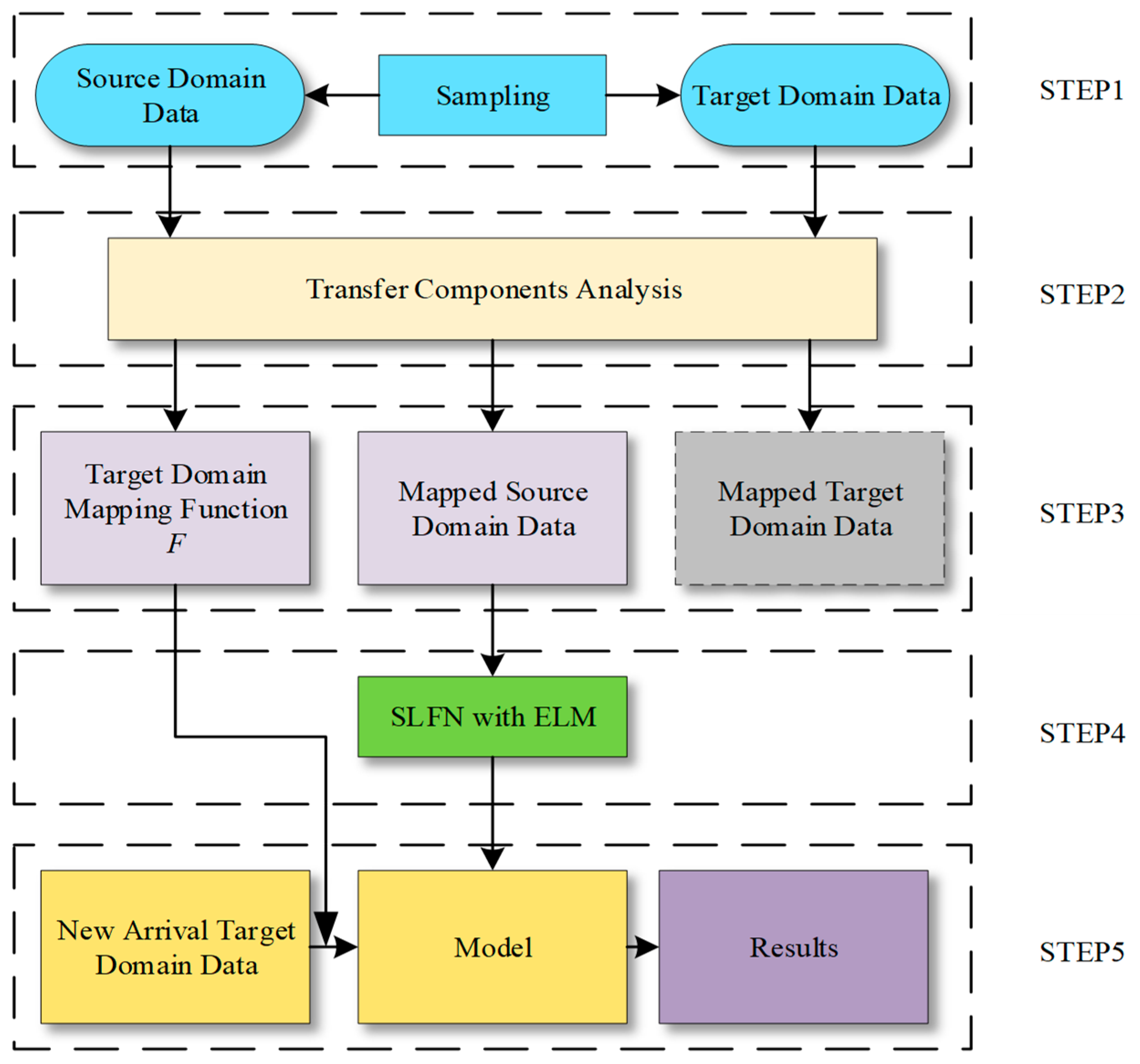
2.3. Framework for Prediction

In this section, the first part is used to discuss the feasibility of this work. In the second part, the proposed framework shown in Figure 6 will be illustrated step by step.
Wu et al. [16] applied IS as a feature selection scheme, which extracts data from the charging voltage. Because the duration is relatively long during the charging operation, it is convenient to be measured, and the curve is relatively stable. It is reliable and relevant to select the feature data from the data of the charging voltage. Therefore, IS is chosen as the feature selection scheme in this paper. The specific selection scheme is shown in Figure 3. The voltage values are selected as the feature data in the ratio of 1/3, 1/2, 2/3, 13/18, 7/9, 5/6, 8/9, 33/36, 17/18, and 35/36 at each charging voltage curve.
Although each battery has different capacity degradation curves, these curves are in a similar degradation pattern. Also, most importantly, the charging curves of different batteries are similar when the number of cycles is different. Namely, the distribution of feature data is similar, but the values are different, which is shown in Figure 4 and Figure 5. This satisfies the premise of feature-based DA [17]. Therefore, it is possible and valid to predict the SOH of the target battery by taking advantage of different types of batteries through the domain adaptation technique.
DA corrects the distribution of source and target domain data essentially and keeps the target domain and source domain data distribution consistent but differential [19]. After this processing, the data of the source domain can be regarded as the same distributed data with target domain data under the new feature space. Hence, these kinds of data can be used as a training set to train a model of machine learning. After that, the ELM algorithm is used as the neural network training algorithm to train a triple layer FFNN because of its extreme fast training speed. Eventually, the source domain data are used as the training set, and the rest of the target domain data are used as the test set to prove the validity of the proposed framework through experiments.
As shown in the framework of Figure 6, the deployment of the algorithm will be explained step by step.
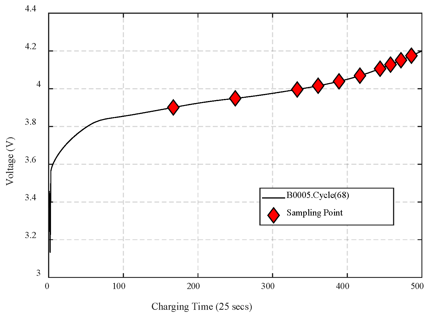
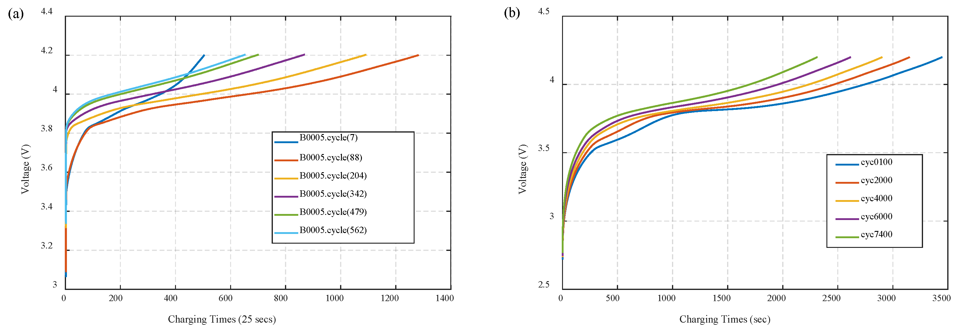
  • To begin with, the complete degradation data of source battery and the previous parts of the target battery data are needed. Features are extracted from the raw data of charging voltage of batteries according to the scheme of IS. As is shown in Figure 4, the data in the middle and posterior parts, especially the latter part, have relatively large differences.
  • The employment of the TCA algorithm is shown in this step. The calculation process of TCA is shown in Section 2.1. First, the input are two feature matrices from source and target domains. Then, calculate the L and H matrices according to Equation (5) and Equation (9). Then, we need to choose a kernel function to calculate the K matrix. In this paper, the Gaussian kernel function in the radial basis function (RBF) is chosen, for its lower computational cost and shorter computation time.
    K ( x , y ) = e ( x y 2 2 σ 2 ) x , y s r c , t a r ,
    where σ is the bandwidth of the Gaussian kernel function.
    Then, the ranked top dth eigenvalues of ( K L K + μ I ) 1 K H K are the source and target domain data we need.
  • After TCA processing, the mapped source domain data, the mapped target domain data, and the function used to map the new arrival target domain data are obtained. Among them, the labels of mapped target domain data remain unknown, because the SOH of target battery is unable to obtain at this moment. For this sack, this part of the data is not used. On the other hand, the source domain data are complete after being mapped. Therefore, it can be used to train an effective model.
  • In this step, an SLFN model based on the ELM training algorithm described in Section 2.2 is trained. In this paper, the activation function of the hidden layer is a sigmoid function:
    g ( x ) = 1 1 + e x .
    For any one of the mapped source domain sample data, it can be formulated as follows:
    x i = [ x i 1 , x i 2 , x i j , , x i n ] n = 1 , 2 , 3 , , d .
    Because of the regression problem, the output of the network has only one neural node and the output is the predicted value. Then, in the context of our application of ELM to predict lithium battery SOH, the output layer only needs one output neuron y i . It can be given as follows:
    y i = j = 1 M β j g ( p = 1 n x i p w p j + b j ) i = 1 , 2 , 3 , ,
    where M is the number of hidden layer neurons in the SLFN and needs to be manually selected.
  • In this step, new arrival target domain data are predicted by a formerly well-trained model. The trained model has different numbers of input neurons with target domain data. Therefore, new arrival target domain data should be mapped by TCA. In an experimental environment, the data sets in use have integrated data of both the source domain and target domain, which can be mapped together by TCA at once. However, in the actual application process, this is not feasible. The newly generated target domain data need to be mapped into the new space by the mapping function F in STEP3. After the new data are mapped to previous latent space, the model can be used to get the desired SOH predictions.

3. Battery Datasets and Experimental Setup

In order to verify the validity of the proposed framework, experiments are proposed for simulation and verification in this section. The experimental platform is Matlab2017a and the computer system is Windows 10. The data sets used in the experiments in this paper are Battery Data Set in PCoE Datasets, provided by The Prognostics Center of Excellence (PCoE) at NASA’s Ames Research Center for fault prediction and diagnostic studies [23]. Battery Data Set has battery degradation data under various operating conditions. In order to ensure the similarity of battery data in different datasets, they are collected under similar charging and discharging conditions. Therefore, in the Battery Data Set, sub-datasets B0005 and B0007 were selected as the experimental data. The two sub-data sets were collected at room temperature for battery #5 and #7, respectively. They were charged to 4.2 V in a 1.5 A constant current mode and then continuously charged at 20 mA. Discharge was implemented at a constant current of 2 A until voltage fell to 2.7 V and 2.2 V [23].
Data are collected at each cycle. These two data sets contain various types of data, such as voltage, current, time data, and impedance data collected in a lithium-ion battery aging experiment. Among these parameters, only the voltage data during the charging process were used in this paper. In Battery Data Set, the EOL of batteries are at 70% capacity. Capacity degradation curves are shown in Figure 7.
On the other hand, Oxford Battery Degradation Dataset 1 is another battery data set in use. This data set is collected in long term battery ageing tests of 8 Kokam (SLPB533459H4) 740 mAh lithium-ion pouch cells [24]. This dataset contains eight sets of sub-data sets that are tested under the same charge and discharge conditions for the same eight pieces of lithium battery at 40 degree centigrade. Charging is carried out at a constant current and constant voltage mode; data are collected every 100 cycles. There are approximately 4500 or 8000 cycles in the sub-data sets.
In Oxford Battery Degradation Dataset 1, the end of life (EOL) of the battery is 75% of the initial capacity.
It can be distinctly seen in Figure 7 that the capacity degradation curve of Cell1, Cell3, Cell7, and Cell8 is similar. The same is true for other types of data of these batteries. They are a better choice than others.
Considering that the EOL of the battery in PCoE Datasets and Oxford Battery Degradation Dataset 1 is discriminate, and the number of cycles is also different, it is necessary to unify the two data sets. Therefore, data are selected before the capacity fell to 75% in PCoE Datasets.

4. Results and Corresponding Discussion

This section is divided into four parts. Section 4.1 is used to demonstrate the effectiveness of ELM in this predictive task. Section 4.2 is used to demonstrate the validity of the final proposed transfer framework. After proving the validity of the framework, Section 4.3 starts with the data and simply explores how the data can improve the accuracy of the prediction. In Section 4.4, explore the impact of the amount of battery data in the target domain on the prediction results. More data means a deeper degradation of the target battery.
The criteria for evaluating the error are mean absolute error (MAE) and root mean squared error (RMSE). The expressions are as follows:
M A E = 1 m i = 1 m | y i y i ^ | ,
R M S E = i = 1 m ( y i y i ^ ) 2 m .

4.1. ELM Effectiveness Experiments

There are four sets of repeated experimental sub-data sets in Oxford Battery Degradation Dataset 1. This data set meets the same data distribution requirements of traditional machine learning. Therefore, this data set is used to verify the validity of the ELM algorithm on this issue. The same is true for selected PCoE data sets.
An ELM model is trained using all stages of Cell1 and then the latter part of Cell3, Cell7, and Cell8 is used as the test set. The experimental results are shown in Table 1 and Figure 8a. In Figure 8c,d, the same experiments are carried out in the PCoE dataset. The experimental results on these two data sets prove that ELM has good ability for this prediction task. In Figure 8b, it is shown that if only the first half of the data is used to train the network, it is hard to train a network that can predict SOH. The testing set used is also from Cell1.

4.2. Transfer Experiment

In this section, the PCoE dataset and Oxford Battery Degradation Dataset 1 serve as the source and target domains, respectively, to demonstrate the validity of the framework.
Because of the randomness of ELM, it is rational to take the average value of 100 experiments under the same settings as the prediction result. Although it is 100 loops, the total time cost of the calculation is less than 1 second.
The categorical results are shown in Table 2, Table 3, and Figure 9. Table 2 shows the prediction results of Battery #05 as the source domain and the others as the target domain. Similar to Table 2, Table 3 shows the prediction results when Battery #07 is used as the source domain. Furthermore, Figure 9 shows some of the results in Table 2. These experimental results prove that the proposed framework is effective. For the fairness of this experiment, in this experiment, the dimension of the TCA was fixed at five dimensions, and the number of neurons in the ELM hidden layer was fixed at 4. These two parameters can be selected in this neighborhood.
The following conclusions can be drawn by comparing Figure 8a with Figure 9a,b. As shown in Table 1, the MAE of experiments in Figure 8a is 1.59% and the RMSE is 3.19%. As shown in Table 2, the MAE of experiments in Figure 9a is 2.10% and the RMSE is 3.51%. This means that the knowledge transferred from other datasets can achieve an accurate prediction of lithium batteries of different types or working conditions for target batteries.

4.3. Discussion of PCoE Dataset

In Figure 5a,b, it is observed that in Battery #05 and #07, approximately the top 20% of the data distribution is significantly different. This experiment is carried out for the discussion of whether the top 20% of the data will result in a worse model. The results of reduced Battery #05 for Cell1 dataset SOH prediction are shown in Figure 10.
A conclusion can be drawn from comparison between the MAE and MSE recorded in Figure 8c and Figure 10. In the case of using Battery #05 to predict the SOH of Cell1, the MAE has dropped 0.45%, about 21.4%. The results of the other datasets also declined about 20%. This means that it is advantageous to do data screening in this work.

4.4. Percentage of Mapping Data

In this part, the proposed experiments are to show the change in the final predicted result using the different percentage of data of battery life as the target domain. Data of Battery #05 are selected as the source domain and data of Cell1 are selected as the target domain. The results are shown in Table 4.
As the target domain data are getting abundant, the overall trend of the forecast results is getting better and better. However, the target domain data cannot be increased arbitrarily. Predicting the battery’s SOH will become meaningless when 90% of the battery’s useful life has been used.

5. Conclusions

Because of the similarity of feature data distribution of charge voltage in different types of batteries, TCA is introduced to take advantage of similar knowledge hidden in the source domain. Moreover, because the mapping function F used for mapping can also handle new arrival data, the proposed framework can do online processing. The result of utilizing B0005 to predict the SOH of Cell1 can achieve a MAE of 1.65% and a RMSE of 2.84%. This shows that it is possible to utilize distinct domain battery data to predict the target domain battery SOH, and the prediction results are accurate. As a conclusion, the main contribution of this paper are as follows:
(1) The ELM training algorithm is used instead of BPNN. This replacement greatly simplifies the computational complexity and improves the model training speed without sacrificing prediction accuracy.
(2) In combination with the TCA, a framework is proposed that is able to predict the SOH of the target battery by using the degradation data of other batteries. When the battery is only used for 30% of its life, it can be predicted to some extent.

Author Contributions

This work was carried out in collaboration between all authors. B.J. proposed and validated this model. Y.G. provided the necessary battery data and added the diversity of the experiment. L.W. provided the necessary help for the implementation of the experiment setup.

Acknowledgments

This work received financial support from the National Natural Science Foundation of China (No.61873175, No.71601022), the Key Project B Class of Beijing Natural Science Fund (KZ201710028028), and the Beijing youth talent support program (No.CIT&TCD201804036). The work was also supported by Youth Innovative Research Team of Capital Normal University.

Conflicts of Interest

The authors declare no conflict of interest.

References

  1. Xiong, R.; Cao, J. Critical review on the battery state of charge estimation methods for electric vehicles. IEEE Access 2018, 6, 1832–1843. [Google Scholar] [CrossRef]
  2. Hossain, L.S.; Hannan, M.A. A review of state of health and remaining useful life estimation methods for lithium-ion battery in electric vehicles: Challenges and recommendations. J. Clean. Prod. 2018, 205, 115–133. [Google Scholar]
  3. Watrin, N.; Blunier, B. Review of adaptive systems for lithium batteries State-of-Charge and State-of-Health estimation. In Proceedings of the 2012 IEEE Transportation Electrification Conference and Expo (ITEC), Dearborn, MI, USA, 18–20 June 2012. [Google Scholar]
  4. Zhang, J.; Lee, J. A review on prognostics and health monitoring of Li-ion battery. J. Power Sources 2011, 196, 6007–6014. [Google Scholar] [CrossRef]
  5. Zheng, X.; Fang, H. An integrated unscented kalman filter and relevance vector regression approach for lithium-ion battery remaining useful life and short-term capacity prediction. J. Rel. Eng. Syst. Saf. 2015, 144, 74–82. [Google Scholar] [CrossRef]
  6. Mingant, R.; Bernard, J. Novel state-of-health diagnostic method for Li-ion battery in service. J. Appl. Energy 2016, 183, 390–398. [Google Scholar] [CrossRef] [Green Version]
  7. Zhang, F.; Liu, G.J. Battery state estimation using unscented kalman filter. In Proceedings of the 2009 IEEE International Conference on Robotics and Automation, Kobe, Japan, 12–17 May 2009; pp. 1863–1868. [Google Scholar]
  8. Fang, L.; Li, J. Online Estimation and Error Analysis of both SOC and SOH of Lithium-ion Battery based on DEKF Method. Energy Procedia 2019, 158, 3008–3013. [Google Scholar]
  9. Andre, D.A.; Christian, S.G. Advanced mathematical methods of SOC and SOH estimation for lithium-ion batteries. J. Power Sources 2013, 224, 20–27. [Google Scholar] [CrossRef]
  10. Hannan, M.A.; Lipu, M.H. Neural Network Approach for Estimating State of Charge of Lithium-ion Battery Using Backtracking Search Algorithm. IEEE Access 2018, 6, 10069–10079. [Google Scholar] [CrossRef]
  11. Civicioglu, P. Backtracking search optimization algorithm for numerical optimization problems. Appl. Math. Comput. 2013, 219, 8121–8144. [Google Scholar] [CrossRef]
  12. Jungsoo, K.; Jungwook, Y. Estimation of Li-ion Battery State of Health based on Multilayer Perceptron: As an EV Application. IFAC-PapersOnLine 2018, 51, 392–397. [Google Scholar]
  13. Zhiwei, H.; Mingyu, G. Online state-of-health estimation of lithium-ion batteries using Dynamic Bayesian Networks. J. Power Sources 2014, 267, 576–583. [Google Scholar]
  14. Zhang, Y.; Xiong, R. Long short-term memory recurrent neural network for remaining useful life prediction of lithium-ion batteries. IEEE Trans. Veh. Technol. 2018, 67, 5695–5705. [Google Scholar] [CrossRef]
  15. Liu, J.; Saxena, A. An adaptive recurrent neural network for remaining useful life prediction of lithium-ion batteries. In Proceedings of the Annual Conference of the Prognostics and Health Management Society, Portland, OR, USA, 10–16 October 2010. [Google Scholar]
  16. Wu, J.; Zhang, C. An online method for lithium-ion battery remaining useful life estimation using importance sampling and neural networks. Appl. Energy 2016, 173, 134–140. [Google Scholar] [CrossRef]
  17. Wang, M.; Deng, W. Deep Visual Domain Adaptation: A Survey. J. Neurocomput. 2018, 312, 135–153. [Google Scholar] [CrossRef]
  18. Weiss, K.; Khoshgoftaar, T.M. A survey of transfer learning. J. Big Data 2016, 3, 9. [Google Scholar] [CrossRef]
  19. Pan, S.J.; Kwok, J.T. Transfer Learning via Dimensionality Reduction. In Proceedings of the 23rd National Conference on Artificial Intelligence (AAAI’08), Chicago, IL, USA, 13–17 July 2008. [Google Scholar]
  20. Schölkopf, B.; Smola, A. Nonlinear component analysis as a kernel eigenvalue problem. J. Neural Comput. 1998, 10, 1299–1319. [Google Scholar] [CrossRef]
  21. Huang, G.B.; Zhu, Q.Y. Extreme learning machine: A new learning scheme of feedforward neural networks. In Proceedings of the 2004 IEEE International Joint Conference on Neural Networks (IEEE Cat. No.04CH37541), Budapest, Hungary, 25–29 July 2004. [Google Scholar]
  22. Huang, G.B. Learning capability and storage capacity of two-hidden-layer feedforward networks. IEEE Trans. Neural Netw. 2003, 14, 274–281. [Google Scholar] [CrossRef] [PubMed]
  23. Saha, B.; Goebel, K. “Battery Data Set”, NASA Ames Prognostics Data Repository. Available online: https://ti.arc.nasa.gov/tech/dash/groups/pcoe/prognostic-data-repository/#battery (accessed on 27 June 2019).
  24. Birkl, C. Oxford Battery Degradation Dataset 1. University of Oxford. Available online: https://ora.ox.ac.uk/objects/uuid:03ba4b01-cfed-46d3-9b1a-7d4a7bdf6fac (accessed on 27 June 2019).
Figure 1. Schematic diagram of transfer component analysis (TCA).
Energies 12 02524 g001
Figure 2. An example of the extreme learning machine (ELM) model.
Energies 12 02524 g002
Figure 3. An example of importance sampling (IS) in charging voltage.
Energies 12 02524 g003
Figure 4. (a) Charging curve of different cycle times in Battery#05. (b) Charging curve of different cycle times in Cell2.
Energies 12 02524 g004
Figure 5. Comparison of (a) first and (b) fifth feature. The first feature refers to the voltage value at 1/3 of the battery during each charge, and the fifth feature is the voltage at 5/9. This means that although the battery data sets are different, the charging voltage has a similar distribution during the charging process of the battery.
Energies 12 02524 g005
Figure 6. Framework for lithium battery prediction. SLFN—single hidden layer feed forward neural network.
Energies 12 02524 g006
Figure 7. (a) The capacity curve of Prognostics Center of Excellence (PCoE) battery data sets #05, #07. (b) The capacity curve of Cell1-Cell8 in Oxford Battery Degradation Dataset 1.
Energies 12 02524 g007
Figure 8. (a) All of Cell1 is used as the training set and rest half of Cell3 is used as testing data. (b) The former half of Cell1 is used as the training set and other half of Cell3 is used as testing data. (c) Integral data of Battery #05 are used as the training set and other half of Battery #07 is used as the testing set; the mean absolute error (MAE) is 2.13% and the mean squared error (MSE) is 3.80%. (d) Integral Battery #07 data is the training set and the other half of Battery #05 is used as the testing set; the MAE is 2.52% and the MSE is 4.12%. SOH—state of health.
Energies 12 02524 g008
Figure 9. (a) Predicting the state of health (SOH) results of Cell1 using integral data of Battery #05. (b) Predicting the SOH results of Cell8 using integral data of Battery #05.
Energies 12 02524 g009
Figure 10. Reduced Battery #05 for Cell1 SOH prediction, the MAE of this result is 1.65% and the RMSE is 2.84%.
Energies 12 02524 g010
Table 1. Testing the reliability of extreme learning machine (ELM) models using similar data sets. MAE—mean absolute error; RMSE—root mean squared error.
Training Set
Test Set
Cell1
Cell3
Cell1
Cell7
Cell1
Cell8
MAE1.59%2.57%2.67%
RMSE3.19%4.62%4.53%
Table 2. Prediction results between Battery #05 and Cell1, Cell3, Cell7, and Cell8.
Source Domain
Target Domain
#05
Cell1
#05
Cell3
#05
Cell7
#05
Cell8
MAE2.10%2.39%1.79%1.98%
RMSE3.51%3.88%3.29%3.65%
Time Cost (s)0.03070.02860.02740.0283
Table 3. Prediction results between Battery #07 and Cell1, Cell3, Cell7, and Cell8.
Source Domain
Target Domain
#07
Cell1
#07
Cell3
#07
Cell7
#07
Cell8
MAE1.87%2.08%1.78%2.65%
RMSE3.16%3.39%3.62%4.83%
Time Cost (s)0.02870.02840.02850.0307
Table 4. Prognosis results for different percentages of target domain data.
Percentage30%
(24/78)
35%
(27/78)
40%
(31/78)
45%
(35/78)
50%
(39/78)
55%
(43/78)
60%
(47/78)
MAE3.40%3.60%2.83%2.86%2.07%1.95%1.47%
RMSE5.27%5.66%4.62%4.81%3.71%3.56%2.84%

