Abstract
Line loss rate plays an essential role in evaluating the economic operation of power systems. However, in a low voltage (LV) distribution network, calculating line loss rate has become more cumbersome due to poor configuration of the measuring and detecting device, the difficulty in collecting operational data, and the excessive number of components and nodes. Most previous studies mainly focused on the approaches to calculate or predict line loss rate, but rarely involve the evaluation of the prediction results. In this paper, we propose an approach based on a gradient boosting decision tree (GBDT), to predict line loss rate. GBDT inherits the advantages of both statistical models and AI approaches, and can identify the complex and nonlinear relationship while computing the relative importance among variables. An empirical study on a data set in a city demonstrates that our proposed approach performs well in predicting line loss rate, given a large number of unlabeled examples. Experiments and analysis also confirmed the effectiveness of our proposed approach in anomaly detection and practical project management.
1. Introduction
Line loss is the power loss of a power grid, which reflects the plan, design, and economic operation level in the power grid. It is also one of the key assessment indicators for a power grid company. The LV distribution network, which is treated as the foundation of line loss management, is now facing the problem of large number, weak management, and poor data quality. At the end of December 2018, the China Southern Power Grid realized 100% coverage of smart meters and automatic meter reading (AMR), making it more objective and accurate when collecting remote data and, thereby, solving the problem of different periods of supply and sale. Currently, the Guangxi Power Grid uses the approach based on measured value to calculate line loss rate. However, it appears that the accuracy is quite low, thus, it is not conducive to analyze line loss. As a result, there is an immense need for algorithms that can carry out a fast and accurate calculation of line loss rate in the LV distribution network.
Currently, there are many approaches to calculate line loss rate, such as traditional based [1], power flow based [2,3], and AI algorithms based approaches [4,5,6,7,8,9,10,11,12,13,14,15,16,17,18,19]. Traditional approaches mainly include the average current method and equivalent resistance method, which simplify the grid structure through a series of assumptions at the cost of sacrificing calculation accuracy. Methods based on power flow, such as the Newton–Raphson method, front push back, are more accurate, but it takes both time and manpower to collect massive operational and structural data. In recent years, AI algorithms have been widely used in power systems, providing new approaches to predict line loss rate. Methods based on linear regression have been proposed as an alternative way to calculate line loss rate, which is fast and straightforward when high prediction accuracy is not required. However, determining a regression equation depends heavily on a great deal of data, and it is difficult to fit the complex nonlinear relationships between line loss rate and features, so the prediction accuracy is not high. The artificial neural network (ANN)-based methods [8,9,10,11,12] are most representative, which can be used to fit arbitrary complex functions without constructing a mathematical model. An optimized back propagation neural network (BPNN) method proposed in [11] proved higher accuracy and convergence speed over traditional ANN, but failed to avoid the defects such as overfitting and the local minima problem. There are also methods based on the ensemble learning algorithm [17] and the support vector machine (SVM), as well as its improved algorithms [18,19], etc. Yet, the studies above have common problems. Firstly, they selected the features by engineering experience, which not only lacks theoretical basis but also has an impact on prediction accuracy. Secondly, they did not involve evaluation, correction, and anomaly detection of line loss rate.
The aims of this paper are to distinguish key features that significantly influence line loss rate, and predict line loss rate under the condition that outliers exist. Consequently, we propose a gradient boosting decision tree (GBDT)-based approach to calculate line loss rate in the LV distribution network. First, we select the features by correlation analysis and construct the corresponding database. Second, considering the great difference in grid structure and the numerical dispersion of line loss rate, we use density-based spatial clustering of applications with noise (DBSCAN) to classify the LV distribution network. Finally, we establish GBDT prediction models for each area, assess the prediction results, and revise the outliers. Rationality and effectiveness have been verified through the analysis of the data set in a city and the comparison among other algorithms. What is more, the prediction accuracy can be significantly improved.
2. Gradient Boosting Decision Tree
2.1. Gradient Boosting
Gradient boosting is an integrated algorithm, which can be used for regression, classification, and ranking problems [20]. It is typically used with decision trees of a fixed size as base learners. Gradient boosting constructs a strong learner by integrating multiple weak learners to build a prediction model, and trains many models in a gradual, additive, and sequential manner. The principle idea of this algorithm is to construct new base learners which can be maximally correlated with negative gradient of the loss function. Different from the traditional boosting algorithm, each new model of gradient boosting is established to reduce the loss function of the previous model along the direction of the gradient. The loss function is used to evaluate the performance of the model—the smaller the loss function is, the better the performance obtained. Gradient boosting is actually doing a form of gradient descent, therefore, in order to keep the performance of the model improved, the best way is to lower the loss function along the direction of gradient descent.
2.2. Classification and Regression Tree
Classification and regression trees (CART) is one of the most well-established machine learning techniques, first introduced by Breiman in 1984 [21]. CART is a typical binary tree, its essence is to divide the feature space into two parts and split the scalar attribute and the continuous attribute [22,23,24,25,26]. The CART algorithm consists of the following two steps: (1) Generate decision tree. This is done via training data set, build nodes from top to bottom. In order to make the resulting child nodes as pure as possible, split each node according to the best attribute. For the classification problem, use GINI value as the basis for splitting node; for the regression problem, use the smallest variance instead. (2) Pruning. A technique that improves predictive accuracy by reducing overfitting and includes pre-pruning and post-pruning. Pre-pruning is to terminate the growth of the decision tree in advance in the process of constructing the decision tree to avoid excessive node generation; post-pruning is to allow the tree to grow to its entirety, then trim the nodes in a bottom-up fashion.
2.3. Gradient Boosting Decision Tree
Gradient boosting decision tree (GBDT), also known as multiple additive regression tree (MART), is an iterative decision tree algorithm proposed by Friedman in 1999 [27]. It is a machine learning technique for regression and classification problems, which produces a prediction model in the form of an ensemble of weak prediction models, typically CART. The learning process of the algorithm is to build a gradient-boosted trees classification or regression model based on the feature and response data set, then use the classification and regression model to classify/predict new incoming samples [28,29,30,31]. Each round of iteration produces a weak classifier, and each classifier is trained on the residuals of the previous classifiers. The process of training GBDT is presented in Figure 1. GBDT can handle both continuous and discrete values, and also improves the shortcomings of overfitting. In recent years, GBDT has been applied in power systems, mainly focused on fault diagnosis, load forecasting, and photovoltaic power prediction [32,33,34,35], which are not related to line loss calculation.

Figure 1.
The process of training the gradient boosting decision tree (GBDT).
3. Approach to Calculating Line Loss Rate in the LV Distribution Network Based on GBDT
3.1. Establish Feature Database
There are many features that affect line loss rate such as power supply radius, load rate, and distribution capacity [36]. It is undoubtedly accurate to take all these features as input variables, however, it may cause dimensional disasters. Meanwhile, the complicated nonlinear relationship among these features will increase calculation [37]. Traditional methods for feature selection rely on expert experience, which is somewhat subjective. Hence, it is difficult to identify the key factors that affect line loss rate. However, GBDT can give relative importance and find the nonlinear relationship between features and line loss rate, which can be used as the reference basis for feature selection. The global importance of feature j is measured by its average importance in every single tree:
where M denotes the number of trees. The relative importance of j in a single tree is calculated as follows:
where J denotes the number of the leaf nodes, J-1stands for number of the non-leaf nodes, is the feature associated with node t, and is the reduction in squared loss after t was split. The indicator function 1 (·) has the value 1 if its argument is true; and zero otherwise. The relative importance ranges from 0 to 100.
In order to realize the consistency of feature selection, we filter irrelevant variables with the Spearman correlation coefficient, which assesses how well the relationship between two variables can be described using a monotonic function. It can be computed using the popular formula:
Here, d denotes the difference between two ranks of each observation, and n is the number of samples.
So far, we can jointly determine the contribution of each feature through the analysis of GBDT relative importance and Spearman correlation coefficient. Next, we need to further filter features according to the prediction performance of different feature combinations on GBDT. Here, we use mean squared error (MSE) to evaluate. The ultimate feature database is the feature set that minimizes MSE. The formula is as follows:
where m is the number of samples, is the measured value, and is the predicted value. The smaller the is, the more accurate the prediction results obtained. Calculating jointly extracted features by GBDT relative importance and Spearman correlation coefficient, the feature dimension can be effectively reduced and the workload of collecting data is significantly reduced as well.
3.2. LV Distribution Network Classification Based on DBSCAN
The disadvantage of the traditional k-means algorithm is that the best number of clusters is hard to choose. Moreover, it is susceptible to outliers [38,39]. However, in actual line loss work, unqualified data may be produced in the process of collecting, transferring, and storing data. To address the issue, we applied the DBSCAN algorithm to cluster the data, which can realize anomaly detection [40,41]. DBSCAN is a clustering algorithm that, given a set of points in some space, groups together points that are closely packed together, marking points that lie alone in low-density regions as outliers. It does not need to specify the number of clusters in the data a priori, as opposed to k-means, and can identify noise data while clustering [42,43,44].
Let be the set of data points, where . The DBSCAN algorithm can be abstracted into the following steps:
(a) Input data set. Set the scan radius and the minimum number of samples in the neighborhood MinPts, see [45] for details.
(b) Calculate the normalized Euclidean distance between two points:
where is the standard deviation.
(c) Form a data set of core object. For , find all neighbor points within distance. Points with a neighbor count greater than or equal to MinPts will be marked as core point or visited.
(d) For those core points that are not already assigned to a cluster, create a new cluster. Recursively find all its density connected points and assign them to the same cluster as the core point.
(e) Iterate through the unvisited points in data set. Points that do not belong to any cluster will be treated as outliers or noise.
3.3. Line Loss Prediction of LV Distribution Network Based on GBDT
The GBDT prediction model for line loss rate in LV distribution network is illustrated in Figure 2. The idea of the algorithm is to improve upon the predictions of the previous tree. Predictions of the final model are, therefore, the weighted sum of the predictions made by the previous tree models:

Figure 2.
GBDT prediction model for line loss rate.
In Equation 6, represents the feature vector, m is the number of regression trees, and denotes the prediction result of the ith decision tree.
Let the number of iterations be M and the loss function be . Firstly, let , then initialize the model and find the constant value c that minimizes . When the mth decision tree is built, loop through the following steps:
(a) Calculate the negative gradient of the loss function in current prediction model:
(b) Estimate the regions of leaf nodes to fit the approximation of the residual, here, s is the number of leaf nodes of the mth regression tree.
(c) Estimate the value of each by linear research to minimize the loss function (used to estimate the loss of the model so that the weights can be updated to reduce the loss on the next evaluation) L, given the current approximation :
(d) Update the model:
where is the learning rate, is the indicator function—that is, take 1 when belongs to ; otherwise take 0. Therefore, we obtain after cycling. Put the variable into and we can then get the predicted line loss rate.
Since GBDT is a serial computing model, it is challenging to carry out parallel computing. Therefore, in this paper, we normalize GBDT with a subsample, which ranges from 0 to 1. This approach is called stochastic gradient boosting tree (SGBT) [46]. At each round of iteration, a subsample of training data is drawn at random from the full training dataset. The randomly selected subsample is then used, instead of the full sample, to fit the base learner. In this way, the GBDT model can be partially paralleled, thereby reducing model overfitting to a certain extent.
The process of predicting line loss rate in the LV distribution network based on GBDT is shown in Figure 3:

Figure 3.
Process of predicting line loss rate based on GBDT.
(a) Data preprocessing. In this step, we deal with data in the LV distribution network, mainly to standardize the data.
(b) Establish a feature database. Extract features by Spearman correlation coefficient and GBDT relative importance, and choose the feature set that minimizes the average error of the model as the final feature database.
(c) Fitting GBDT model. Train the GBDT model and tune hyperparameters, then verify and evaluate the model by cross-validation.
(d) Predict line loss rate and analyze the results. Input the data into the model and compare it with other algorithms in the aspect of relative error.
4. Experiments
In order to verify the effectiveness of our proposed approach, we take the data of the LV distribution network as an example. We select 1434 pieces of samples from the line loss management system and measurement automation system, each sample includes six independent variables and one dependent variable. The independent variables include power factor, total number of meters, total length of the line, average load rate, main line cross-sectional area, and power supply. The dependent variable is the line loss rate.
4.1. Data Preprocessing
Due to the influence of various factors such as measurement, marketing, and equipment maintenance, the data quality in the LV distribution network is poor, thus, it inevitably generates outliers. Therefore, we detect outliers and missing values by DBSCAN, as described in Step e), Section 2.2. The anomaly detection depends on scan radius , the minimum number of samples included in the neighborhood , and the distance metric we select. In this paper, we choose the Euclidean distance. The formula is as follows:
where is the Euclidean distance between and .
Since GBDT builds one decision tree at a time to fit the residual of the loss function, in order to avoid the instability of the parameters that fit the negative gradient at each iteration. Data are normalized by Z-score, which is calculated as
where is the mean of the population and is the standard deviation of the sample.
4.2. Establish Feature Database
Firstly, we select the electrical features that are normally accessible and best reflect the grid and load characteristics [47]. Considering the accessibility of the data, we choose six mainstream indicators. Using GBDT relative importance and Spearman correlation coefficient to evaluate feature contribution. The result is shown in Figure 4.

Figure 4.
Contribution of each feature. (a) Spearman’s rank correlation coefficient, and (b) GBDT relative importance.
From Figure 4a,b we can see that the power supply and the main line cross-sectional area are always the important features, the rankings of other features are changed where the power factor is always low-scoring. Consequently, we can say that the relative importance of GBDT and the Spearman correlation coefficient have obtained consistency, thereby we can filter the power factor. We then put the data sets that contain different numbers of features into the model, then calculate MSE, respectively. The result is displayed in Figure 5. The value of MSE fell to a low point of 2.058 when the number of features was 4, which means the prediction performance is the best, at this point. Therefore, the best number of features is 4.
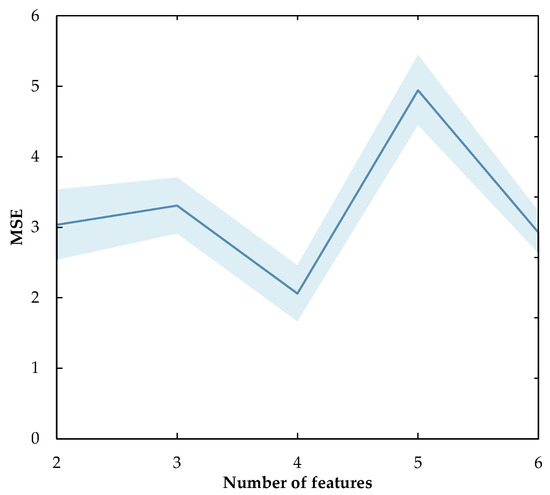
Figure 5.
Mean squared error (MSE) for different number of features.
4.3. Classifying the LV Distribution Network
Due to the different structure and management level in the LV distribution network, electrical features vary greatly in value. Here, we use DBSCAN to classify the LV distribution network and calculate the cluster center of each feature. The results are shown in Table 1.

Table 1.
Cluster center of each feature.
From Table 1, we can conclude the characteristics in each type of LV distribution network. For instance, type A indicates the area where the main line cross-sectional area, the total length of the line, and the power supply area is large, which is contrary to type D. In summary, we can see that each type of LV distribution network has its practical significance, respectively, indicating that the clustering effect is quite good. It should be noted that line aging, line diameter, and transformer upgrade will lead to large fluctuations in line loss rate, so it is normal that the clustering result would correspondingly change.
4.4. Results
In this paper, we use 10-fold cross-validation to estimate the performance of the model, which is primarily used in applied machine learning to estimate the skill of a machine learning model on unseen data. This approach involves randomly dividing the set of observations into ten folds of approximately equal size. The first fold is treated as a validation set, and the method is fit on the remaining nine folds [48], ensuring that each fold is used as a testing set at some point. We then evaluate the model performance based on an error metric.
Figure 6 shows the process of building a gradient decision tree. We assume that the main line cross-sectional area, the total length of the line, the power supply, and the average load rate are , , , and , respectively. For ease of explanation, we limit the maximum depth as 2. The regression tree is characterized by , i.e., the total length of the line. We selected the smallest cut-point of MSE as the optimal cut-point. Samples with a variable less than or equal to the cut-point are divided into the left subtree; otherwise, they belong to the right subtree. For example, when = 1000, after traversing the regression tree, the predicted value is 6.165, i.e., the average line loss rate of 126 samples, where MSE is 3.404.
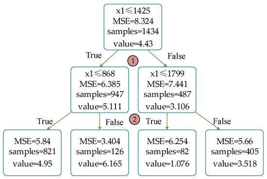
Figure 6.
Process of building a gradient decision tree.
We set the value of subsample as 0.8, which means 80% of the samples are used to fit the individual base learners in every single iteration. Here, we divide samples into the training set and testing set, at a ratio of 9:1. Figure 7 shows the changes in algorithmic errors on training and testing set as the epoch increases. Here, we measured the error by MSE. The dotted line marks the beginning of the overfit. When the epoch of base learner reaches 140, the loss on the training set and testing set track each other rather nicely, and the model on the testing set (subsample = 0.8) would be best predictive and fitted while testing error starts climbing upwards (subsample = 1). At this point, the MSE on testing set is 1.492, which means the model would perform better on new data. In this paper, we compare GBDT with support vector regression (SVR) and random forest (RF) in the aspect of prediction accuracy. In order to quickly find optimal parameters, we use GridsearchCV to tune parameters, which does not need to loop over the parameters and runs all the combinations of parameters. Hyperparameters for each model are presented in Table 2.

Figure 7.
Learning curves for training set and testing set.
Table 2.
Hyperparameters for each model.
For ease of presentation, we showcase the prediction results of three models on one of the testing set in a single iteration, which counts for 115 samples. The comparison of the prediction errors of the three models is shown in Table 1, the prediction and error curves of the three models are displayed in Figure 8a,b. From Figure 8a we can see that the prediction curve of SVR is most deviate from the measured value, next is RF, while the overall trend of the GBDT curve is practically the same as the measured value curve—which is also reflected in Figure 8b. Besides, the average mean squared error of GBDT is reduced by 2.24% and 0.86% compared with SVR and RF, and the maximum relative error is reduced by 16.1% and 9.41%, respectively. In addition, GBDT performs best with the average relative error less than 2%, whereas the average relative error of the other two models is 5 times and 3 times that of GBDT, respectively. Therefore, we can conclude that the overall prediction accuracy of GBDT is higher than SVR and RF.

Figure 8.
Prediction and error curve of three models. (a) Prediction curve for three models, and (b) relative error curve for three models.
Although these algorithms are good at handling various nonlinear problems, in many cases SVR is sensitive to outliers and missing values, while GBDT and RF are not. Both GBDT and RF are ensemble learning methods and predict by combining the outputs from individual trees, yet on our dataset, GBDT proved to be more effective than RF. The reason is that, for data including categorical variables with different numbers of levels (e.g., the total length of the line ranges from hundreds to thousands), random forests are more biased in favor of those attributes with more levels, compared with GBDT. Therefore, the variable importance scores from random forest are not reliable for this type of data, hence the prediction accuracy of RF would be severely affected. In summary, the overall prediction results of GBDT are better than SVR and RF.
We analyze the prediction results in Figure 9, then extract ten samples and estimate their line loss rate, as shown in Table 3. The pie chart presents the percentage of each area in the LV distribution network. To be more specific, area 1 indicates the area where the interval of the measured value is (0,8%) and the relative error is between –5% to 5%, which takes the most of the whole samples (91.40%). We mark this area as ’Qualified’. Area 2—whose measured value greater than 8% with relative error between –5% to 5%—takes up 5.66% of the whole samples, is treated as ’Heavy loss’ as well as key concern, who may have problem with small wire diameter, light load, or long power supply distance. Therefore, there is significant potential in reducing line loss rate. Area 3, whose line loss rate is negative, missing, or too large, is treated as ’Abnormal’. On the one hand, our approach gives reasonable value as a reference; on the other hand, it should be highly valued by relevant departments, verifying whether the measured value is fair, and determining the source of the error to formulate reasonable measures for reducing line loss rate (Table 4).
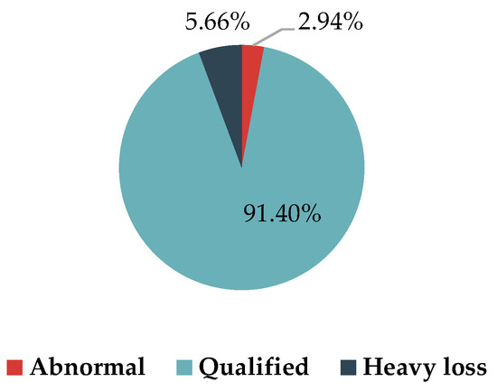
Figure 9.
Analysis on prediction results.
Table 3.
Model prediction error comparison.
Table 4.
Assessment of the LV distribution network.
5. Conclusions
In this paper, we propose a GBDT-based approach to predict line loss rate in the LV distribution network. Effectiveness has been demonstrated by the analysis and verification in the data set of the LV distribution network. First of all, the strength of our approach lies in its high accuracy of predicting line loss rate. In addition, paralleling in a subsample fashion can reduce overfitting to some extent, which overcomes the shortcoming of the original GBDT. Moreover, its good robustness to the outliers and missing values, as well as its partially paralleled design makes it possible to perform better in the process of predicting line loss rate, compared with SVR and RF. We believe that GBDT is of high potential in many application areas, and its use for predicting line loss rate will lead to many follow-up results, and spark new algorithm improvement as well. In summary, our proposed approach suggests that it can be quite useful in practice, specifically, it enables rapid calculation, anomaly detection, and reduction planning of line loss rate, thus effectively improving standardization and management levels in the LV distribution network.
Author Contributions
Conceptualization, Y.Z. and H.W.; methodology, M.Y.; software, M.Y.; validation, M.Y. and J.L.; formal analysis, M.Y.; investigation, M.Y. and P.H.; writing—original draft preparation, M.Y.; writing—review and editing, Y.Z. and H.W.; visualization, J.L.
Funding
This research received no external funding.
Conflicts of Interest
The authors declare no conflict of interest.
Abbreviations
The following abbreviations are used in this manuscript:
| LV | Low voltage |
| GBDT | Gradient boosting decision tree |
| DBSCAN | Density-based spatial clustering of applications with noise |
| AMR | Automatic meter reading |
| ANN | Artificial neural network |
| BPNN | Back propagation neural network |
| SVR | Support vector regression |
| RF | Random forest |
| CART | Classification and regression trees |
| MART | Multiple additive regression tree |
| MSE | Mean squared error |
| SGBT | Stochastic gradient boosting tree |
References
- Sun, D.I.H.; Abe, S.; Shoults, R.R.; Chen, M.S.; Eichenberger, P.; Farris, D. Calculation of Energy Losses in a Distribution System. IEEE Trans. Power Appar. Syst. 1980, PAS-99, 1347–1356. [Google Scholar] [CrossRef]
- Chen, L.I.; Ding, X.Q.; Liu, X.B.; Zhou, Z.H. Line loss comprehensive analytical method based on real-time system data and its application. Electr. Power Autom. Equip. 2005, 25, 47–50. [Google Scholar]
- Li, Z.Y.; Ren, Z.; Chen, Y.J. Loss study of HVDC system. Dianli Zidonghua Shebei/Electr. Power Autom. Equip. 2007, 27, 9–12. [Google Scholar]
- Chen, D.; Guo, Z. Distribution system theoretical line loss calculation based on load obtaining and matching power flow. Power Syst. Technol. 2005, 29, 80–84. [Google Scholar]
- Zhang, K.; Yang, X.; Bu, C.; Ru, W.; Liu, C.; Yang, Y.; Chen, Y. Theoretical analysis on distribution network loss based on load measurement and countermeasures to reduce the loss. Proc. Chin. Soc. Electr. Eng. 2013, 33, 92–97. [Google Scholar]
- Liu, T.; Wang, S.; Zhang, Z.; Zhu, J. Newton-Raphson method for theoretical line loss calculation of low-voltage distribution transformer district by using the load electrical energy. Power Syst. Prot. Control 2015, 43, 143–148. [Google Scholar]
- Xin, K.Y.; Yang, Y.H.; Chen, F. Advanced algorithm based on combination of GA with BP to energy loss of distribution system. Proc. Chin. Soc. Electr. Eng. 2002, 22, 79–82. [Google Scholar]
- Li, X.Q.; Wang, H.; Xu, C.W.; Xu, F.; Zhao, L.N.; Meng, Q.R.; Liu, D.W. Calculation of line losses in distribution systems using artificial neural network aided by immune genetic algorithm. Proc. CSU-EPSA 2009, 37, 36–39. [Google Scholar]
- Jiang, H.L.; An, M.; Liu, X.J.; Zhao, X.; Zhang, J.H. Calculation of energy losses in distribution systems based on RBF network with dynamic clustering algorithm. Proc. Chin. Soc. Electr. Eng. 2005, 25, 35–39. [Google Scholar]
- Kim, H.; Ko, Y.; Jung, K.H. Artificial neural-network based feeder reconfiguration for loss reduction in distribution systems. IEEE Trans. Power Deliv. 1993, 8, 1356–1366. [Google Scholar] [CrossRef]
- Li, Y.; Liu, L.; Li, B.; Yi, J.; Wang, Z.; Tian, S. Calculation of line loss rate in transformer district based on improved k-means clustering algorithm and BP neural network. Proc. CSEE 2016, 36, 4543–4551. [Google Scholar]
- Ahmadizar, F.; Soltanian, K.; Akhlaghiantab, F.; Tsoulos, I. Artificial neural network development by means of a novel combination of grammatical evolution and genetic algorithm. Eng. Appl. Artif. Intell. 2015, 39, 1–13. [Google Scholar] [CrossRef]
- Zou, Y.F.; Mei, F.; Yue, L.I.; Cheng, Y.; Wang, T.U.; Mei, J. Prediction model research of reasonable line loss for transformer district based on data mining technology. Power Demand Side Manag. 2015, 4, 25–29. [Google Scholar] [CrossRef]
- Chen, C.S.; Hwang, J.C.; Cho, M.Y.; Chen, Y.W. Development of simplified loss models for distribution system analysis. IEEE Trans. Power Deliv. 2002, 9, 1545–1551. [Google Scholar] [CrossRef]
- Huang, D.X.; Gong, R.X.; Gong, S. Prediction of Wind Power by Chaos and BP Artificial Neural Networks Approach Based on Genetic Algorithm. J. Electr. Eng. Technol. 2015, 10, 41–46. [Google Scholar] [CrossRef]
- Fushuan, W.; Zhenxiang, H. The Calculation of Energy Losses in Distribution Systems Based upon a Clustering Algorithm and an Artificial Neural Network Model. Proc. CSEE 1993, 3, 41–51. [Google Scholar]
- Wang, S.; Zhou, K.; Yun, S.U. Line loss rate estimation method of transformer district based on random forest algorithm. Electr. Power Autom. Equip. 2017. [Google Scholar] [CrossRef]
- Peng, Y.; Liu, K. A distribution network theoretical line loss calculation method based on improved core vector machine. Proc. Chin. Soc. Electr. Eng. 2011, 31, 120–126. [Google Scholar]
- Xu, R.; Wang, Y. Theoretical line loss calculation based on SVR and PSO for distribution system. Electr. Power Autom. Equip. 2012, 32, 86–89+93. [Google Scholar]
- Breiman, L. Arcing The Edge. Ann. Stat. 1998, 26, 801–824. [Google Scholar]
- Breiman, L.; Friedman, J.; Stone, C.J.; Olshen, R.A. Encyclopedia of Ecology. In Classification and Regression Trees; Routledge: London, UK, 1984. [Google Scholar]
- Seera, M.; Lim, C.P. Online Motor Fault Detection and Diagnosis Using a Hybrid FMM-CART Model. IEEE Trans. Neural Netw. Learn. Syst. 2014, 25, 806–812. [Google Scholar] [CrossRef] [PubMed]
- Gey, S.; Nedelec, E. Model selection for CART regression trees. IEEE Trans. Inf. Theory 2005, 51, 658–670. [Google Scholar] [CrossRef]
- Wang, T.; Pal, A.; Thorp, J.S.; Wang, Z.; Liu, J.; Yang, Y. Multi-Polytope-Based Adaptive Robust Damping Control in Power Systems Using CART. IEEE Trans. Power Syst. 2015, 30, 2063–2072. [Google Scholar] [CrossRef]
- Loh, W.Y. Classification and regression trees. Wiley Interdiscip. Rev. Data Min. Knowl. Discov. 2011, 1, 14–23. [Google Scholar] [CrossRef]
- Zhang, X.; Wang, X.; Chen, W.; Tao, J.; Huang, W.; Wang, T. A Taxi Gap Prediction Method via Double Ensemble Gradient Boosting Decision Tree. Processdings of the 2017 IEEE 3rd International Conference on Big Data Security on Cloud (Bigdatasecurity), Beijing, China, 26–28 May 2017; pp. 255–260. [Google Scholar] [CrossRef]
- Friedman, J.H. Greedy function approximation: A gradient boosting machine. Ann. Stat. 2001, 29, 1189–1232. [Google Scholar] [CrossRef]
- Ma, X.; Ding, C.; Luan, S.; Wang, Y.; Wang, Y. Prioritizing Influential Factors for Freeway Incident Clearance Time Prediction Using the Gradient Boosting Decision Trees Method. IEEE Trans. Intell. Transp. Syst. 2017, 18, 2303–2310. [Google Scholar] [CrossRef]
- Shouxiang W, T.L. Gradient Boosting Decision Tree Method for Residential Load Classification Considering Typical Power Consumption Modes. Proc. CSU-EPSA 2017, 29, 27–33. [Google Scholar] [CrossRef]
- Wang, L.; Zhou, D.; Zhang, H.; Zhang, W.; Chen, J. Application of Relative Entropy and Gradient Boosting Decision Tree to Fault Prognosis in Electronic Circuits. Symmetry 2018, 10, 495. [Google Scholar] [CrossRef]
- Lucas, A.; Barranco, R.; Refa, N. EV Idle Time Estimation on Charging Infrastructure, Comparing Supervised Machine Learning Regressions. Energies 2019, 12, 269. [Google Scholar] [CrossRef]
- Naz, A.; Javed, M.U.; Javaid, N.; Saba, T.; Alhussein, M.; Aurangzeb, K. Short-Term Electric Load and Price Forecasting Using Enhanced Extreme Learning Machine Optimization in Smart Grids. Energies 2019, 12, 866. [Google Scholar] [CrossRef]
- Wang, J.; Li, P.; Ran, R.; Che, Y.; Zhou, Y. A Short-Term Photovoltaic Power Prediction Model Based on the Gradient Boost Decision Tree. Appl. Sci. 2018, 8, 689. [Google Scholar] [CrossRef]
- Cai, L.; Gu, J.; Ma, J.; Jin, Z. Probabilistic Wind Power Forecasting Approach via Instance-Based Transfer Learning Embedded Gradient Boosting Decision Trees. Energies 2019, 12, 159. [Google Scholar] [CrossRef]
- Zheng, H.; Yuan, J.; Chen, L. Short-Term Load Forecasting Using EMD-LSTM Neural Networks with a Xgboost Algorithm for Feature Importance Evaluation. Energies 2017, 10, 1168. [Google Scholar] [CrossRef]
- Ouyang, S.; Chen, X. Reactive power optimal configuration strategy in transformer areas based on normal state-differential characteristics. Power Syst. Technol. 2015, 39, 3513–3519. [Google Scholar] [CrossRef]
- Ouyang, S.; Feng, T.; An, X. Line-loss rate calculation model considering feeder clustering features for medium-voltage distribution network. Electr. Power Autom. Equip. 2016, 36, 33–39. [Google Scholar] [CrossRef]
- Xu, T.; Chiang, H.; Liu, G.; Tan, C. Hierarchical K-means Method for Clustering Large-Scale Advanced Metering Infrastructure Data. IEEE Trans. Power Deliv. 2017, 32, 609–616. [Google Scholar] [CrossRef]
- Mat Isa, N.A.; Salamah, S.A.; Ngah, U.K. Adaptive fuzzy moving K-means clustering algorithm for image segmentation. IEEE Trans. Consum. Electr. 2009, 55, 2145–2153. [Google Scholar] [CrossRef]
- Ghaemi, Z.; Farnaghi, M. A Varied Density-based Clustering Approach for Event Detection from Heterogeneous Twitter Data. ISPRS Int. J. Geo-Inf. 2019, 8, 82. [Google Scholar] [CrossRef]
- Lee, G.; Kim, D.I.; Kim, S.H.; Shin, Y.J. Multiscale PMU Data Compression via Density-Based WAMS Clustering Analysis. Energies 2019, 12, 617. [Google Scholar] [CrossRef]
- Jadidi, A.; Menezes, R.; De Souza, N.; De Castro Lima, A.C. A Hybrid GA–MLPNN Model for One-Hour-Ahead Forecasting of the Global Horizontal Irradiance in Elizabeth City, North Carolina. Energies 2018, 11, 2614. [Google Scholar] [CrossRef]
- Gowanlock, M.; Blair, D.M.; Pankratius, V. Optimizing Parallel Clustering Throughput in Shared Memory. IEEE Trans. Parallel Distrib. Syst. 2017, 28, 2595–2607. [Google Scholar] [CrossRef]
- Shen, J.; Hao, X.; Liang, Z.; Liu, Y.; Wang, W.; Shao, L. Real-Time Superpixel Segmentation by DBSCAN Clustering Algorithm. IEEE Trans. Image Process. 2016, 25, 5933–5942. [Google Scholar] [CrossRef] [PubMed]
- Ester, M.; Kriegel, H.P.; Sander, J.; Xu, X. A Density-Based Algorithm for Discovering Clusters in Large Spatial Databases with Noise. In Proceedings of the KDD’96 Proceedings of the Second International Conference on Knowledge Discovery and Data Mining, Portland, OR, USA, 2–4 August 1996. [Google Scholar]
- Friedman, J.H. Stochastic Gradient Boosting. Comput. Stat. Data Anal. 2002, 38, 367–378. [Google Scholar] [CrossRef]
- Ouyang, S.; Yang, J.; Geng, H.; Wu, Y.; Chen, X. Comprehensive evaluation method of transformer area state oriented to transformer area management and its application. Dianli Xitong Zidonghua/Autom. Electr. Power Syst. 2015, 39, 187–192. [Google Scholar] [CrossRef]
- James, G.; Witten, D.; Hastie, T.; Tibshirani, R. An Introduction to Statistical Learning; Springer: Berlin, Germany, 2013. [Google Scholar]


© 2019 by the authors. Licensee MDPI, Basel, Switzerland. This article is an open access article distributed under the terms and conditions of the Creative Commons Attribution (CC BY) license (http://creativecommons.org/licenses/by/4.0/).