Wind Farm Layout Upgrade Optimization

Abstract

The problem of optimally increasing the size of existing wind farms has not been investigated in the literature. In this paper, a proposed wind farm layout upgrade by adding different (in type and/or hub height) commercial turbines to an existing farm is introduced and optimized. Three proposed upgraded layouts are considered: internal grid, external grid, and external unstructured. The manufacturer’s power curve and a general representation for thrust coefficient are used in power and wake calculations, respectively. A simple field-based model is implemented and both offshore and onshore conditions are considered. A genetic algorithm is used for the optimization. The trade-off range between energy production and cost of energy is investigated by considering three objective functions, individually: (1) annual energy production; (2) cost of added energy; and (3) cost of total energy. The proposed upgraded layouts are determined for the Horns Rev 1 offshore wind farm. The results showed a wide range of suitable upgrade scenarios depending on the upgraded layout and the optimization objective. The farm energy production is increased by 190–336% with a corresponding increase in the total cost by 147–720%. The external upgrade offers more energy production but with much more cost. The unstructured layouts showed clear superiority over the grid ones by providing much lower cost of energy.

1. Introduction

Wind energy has become an increasingly competitive source of electricity, not only among renewable energy sources but also compared with conventional fossil fuels [1]. The global cumulative installed wind capacity exceeded 539 GW by the end of 2017 [2]. Wind power represents about 6% of the global electricity capacity and more than 3% of the global electricity generation of all energy sources [3,4]. Among renewable energy sources, wind energy capacity is more than half the global renewable installed capacity (not including hydropower) [1], it also shares more than half the growth [5]. Wind energy is also the second highest growing renewable energy source (after solar photovoltaics) [1,5]. The 2003–2017 global cumulative installed wind capacity [2] was normalized as a percentage of the 2017 value and presented in Figure 1.

The energy demand for human activities has increased rapidly, which requires energy rationalization for both conventional and renewable energy resources. For wind power, beside the challenging initial cost, the feasible sites for new projects that have promising wind resources are limited. Moreover, wind energy is facing many restrictions because of environmental impact in the form of noise, visual effects, and bird and bat interactions, e.g., [6]. As a result, Wind Farm Layout Optimization (WFLO) became an essential part of wind farm planning, in order to maximize the Annual Energy Production (AEP) and/or minimize the Cost Of Energy (COE) or any undesired environmental impact. The first WFLO study was published in 1994 by Mosetti et al. [7] for a relatively simple problem. The classical era of WFLO extended up to the beginning of the second decade in the 21st century. The wind farms designed in this era are characterized by:

• Identical turbines.
• Relatively low area utilization (large distance among turbines).
• Average tower height, H, of about 80 m [8].
• Average rotor diameter, D, of about 85 m [8].
• Average rated power, P_R, of about 1.8 MW [8].

It is important to mention here that designing, ordering, installing, and testing turbines for a large wind farm takes more than two years, e.g., [9]. This simply means that the majority of the wind farms that have been installed by the end of 2012 were not thoroughly optimized, based on the recent research findings for WFLO. Increasing wind energy production to meet the global demand requires installing new farms. This should be done side by side with enhancing the performance of the existing ones in order to reduce the technical, financial, and environmental challenges facing the installation of new farms.

When a wind farm reaches the end of its useful life (20–25 years) [10], it is commonly either “repowered” or “decommissioned”. An old farm may be repowered or upgraded by replacing some parts (or even some turbines) with more advanced and efficient technology. On the other hand, if the repowering process is found to be infeasible, the whole project is decommissioned by ceasing the power production and dismantling the site, e.g., [11,12,13]. According to Figure 1, less than 7% of the existing farms could benefit from either repowering or decommissioning. However, there is a third scenario when a farm is neither well-optimized according to the recent WFLO findings, nor sufficiently old to be repowered or decommissioned. It is shown in Figure 1 that more than 45% of current farms were installed between 2003 and 2012. Those farms are still in the first half of their lifespan. Accordingly, neither repowering nor decommissioning is feasible, and a new strategy considering upgrading should be taken into account.

The present work aims to investigate the feasibility of upgrading an existing wind farm while keeping the original turbines unchanged. Such a problem we call “wind farm layout upgrade optimization, WFLUO”.

In this paper, the problem of WFLUO is addressed for the first time in the literature. The proposed methodology is applied to Horns Rev 1 offshore wind farm as a case study. In Section 2, the case study is highlighted and justified. The proposed upgrade methodology is given in Section 3. The results and discussions are the topic of Section 4, while the most useful conclusions are listed in Section 5.

2. Horns Rev 1 and Literature Review

Horns Rev 1 is one of the most famous wind farms worldwide. It has received great interest since commencing power production in 2002 for many reasons, which can be summarized as:

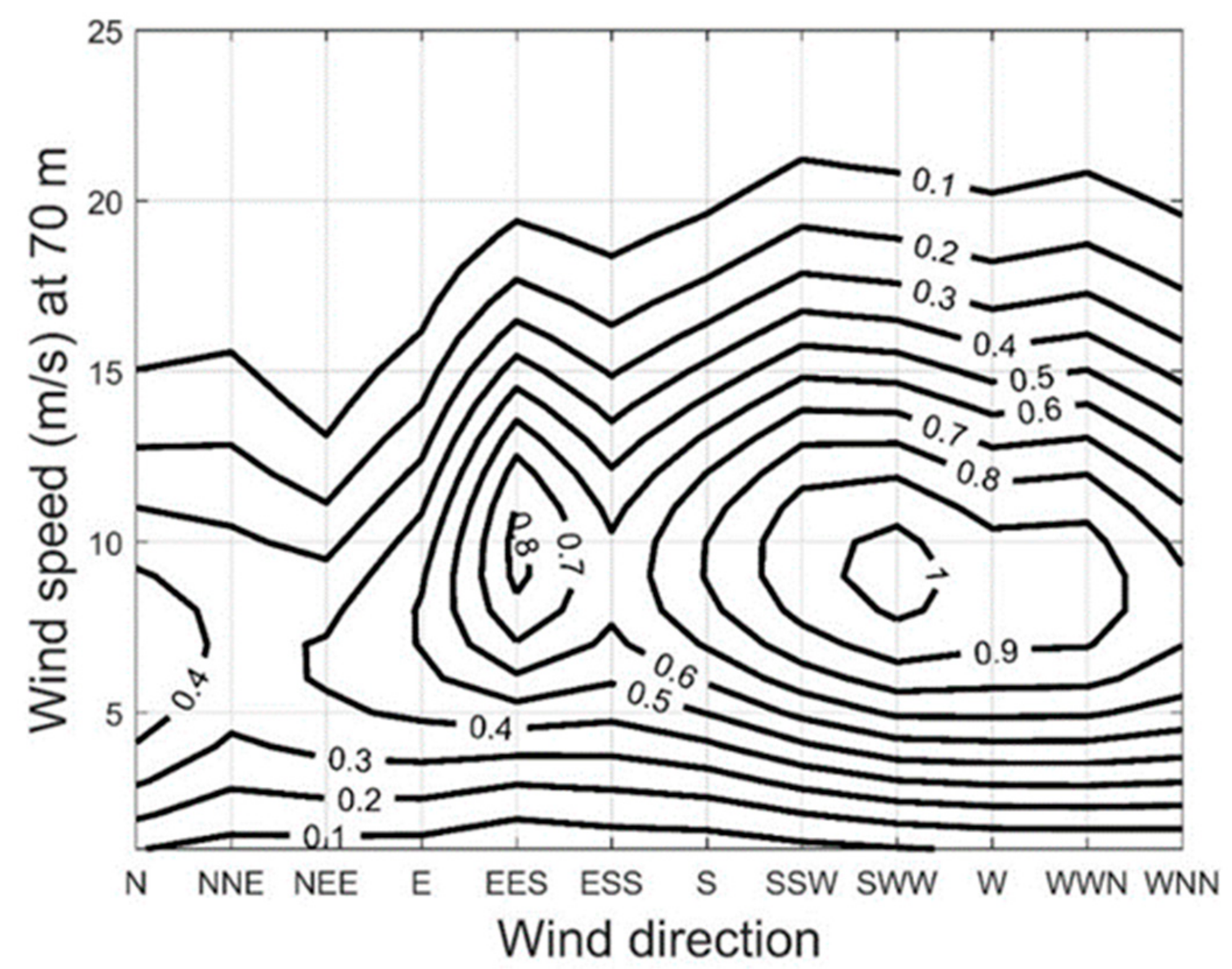
• Three years of detailed wind resource assessment data taken prior to the installation are publicly available [14].
• Detailed operational measurements are also publicly available, e.g., [15].
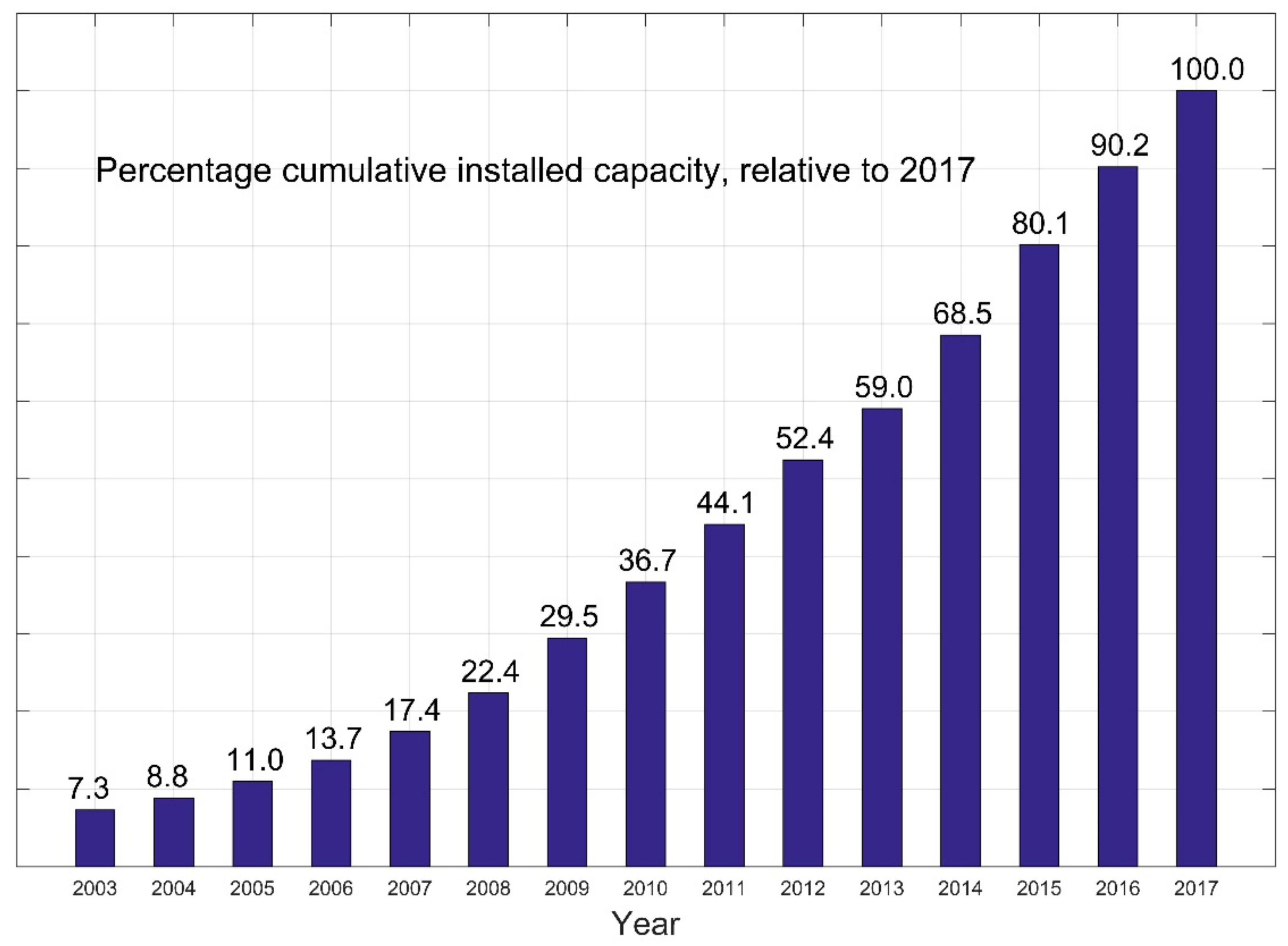
• The installed capacity is 160 MW, which made it the world’s largest offshore wind farm when installed and for several years thereafter.
• Since installed in 2002 it has produced more than 9 TW-hr [16].

Accordingly, the farm performance and wake measurements were used in many wake model validations and wind farm layout optimization studies, e.g., [15,17,18,19,20,21,22]. As mentioned earlier, WFLUO is not found in the literature; however, some relevant studies will be reviewed below.

Huo, et al. [12] applied a proposed repowering optimization strategy on Horns Rev 1 as a case study. They investigated two repowering scenarios, each with two stages four years apart. The results showed that the levelized cost of electricity could be reduced by up to 10.43%. They emphasized that their findings are limited to a specific wind farm, while the method itself should be generally applicable, although it does not address WFLUO.

Many investigators have computationally improved the Horns Rev 1 performance by relocating the turbines within the farm area. Rivas et al. [23] applied the Simulated Annealing Algorithm to the Turbine Positioning Problem in order to maximize the AEP. They concluded that the AEP could be increased up to 1%. Vezyris [24] applied deterministic, semi-stochastic, and stochastic approaches in order to minimize the Levelized Production Cost (cents/kWh). The results showed that a decrease in the Levelized Production Cost by ~1% combined with an increase in the AEP with ~1% could be achieved by re-optimizing the farm layout. Park and Law [25] derived a continuous and smooth wind speed profile that allowed the wind farm power function to be expressed as a smooth (differentiable) function of wind turbine location variables. The wind farm power function then optimized using a gradient-based optimization algorithm. The minimum turbine proximity was fixed at 5 D and the results suggested an increase in the farm output power by 7.3%, without providing with any cost calculations.

Horns Rev 1 wind farm has 80 identical turbines (8 East-to-West rows by 10 North-to-South columns). The northern end of the columns is aligned approximately 7.2° West of North, forming a parallelogram. The turbines are all Vestas V80-2.0 with a rotor diameter of 80 m and rated power of 2 MW. The spacing between turbines in both the rows and columns is 7 D. The tower height is 70 m and the power curve is specific for the turbines delivered to this wind farm and may not apply to other V80 turbines [15].

Apart from the availability of performance and other data that was noted above, Horns Rev 1 was chosen as a case study as an example of middle-aged non-optimized wind farm, based on the recent findings. It is about 15 years old, it contains identical turbines, the turbines’ rated power and hub height are below the recent average values for offshore farms [8], and finally, the turbines spacing is 7 D in both directions, which is significantly larger than in more recent farms.

The references quoted above optimized the farm performance by computationally re-locating the turbines, but this is clearly infeasible for most existing wind farms. This work presents WFLUO, for the first time in the literature, by not changing the existing farm layout, but by adding additional turbines. The proposed methodology is based on commercial turbine selection and hub height variation, which was introduced in [26].

Understanding and analyzing the wind data is an essential task in any wind power project. As mentioned earlier, three years of wind measurements were made prior to Horns Rev 1 installation. The wind data at 62 m height from 1 June 1999 to 31 May 2002 was averaged and the Weibull parameters—scale and shape factors—were evaluated for 12 directional sectors (30 degrees each) [14]. Moreover, these parameters were extrapolated to the hub height of 70 m [27]. Figure 2 shows the frequency of occurrence, f, of each freestream speed (at hub height) at different wind directions in contour format.

3. WFLUO Methodology

The proposed upgrade methodology is described in detail in this section. In Section 3.1, the proposed upgraded layouts are illustrated. The wake model and wake interference calculations are described briefly in Section 3.2. Section 3.3 describes the pool of commercial turbines from which the turbines for the upgraded farm were chosen as well as the AEP calculations. The strategy of hub height variation is discussed in Section 3.4. Finally, the cost analysis and the optimization methodology are the topics of Section 3.5 and Section 3.6, respectively.

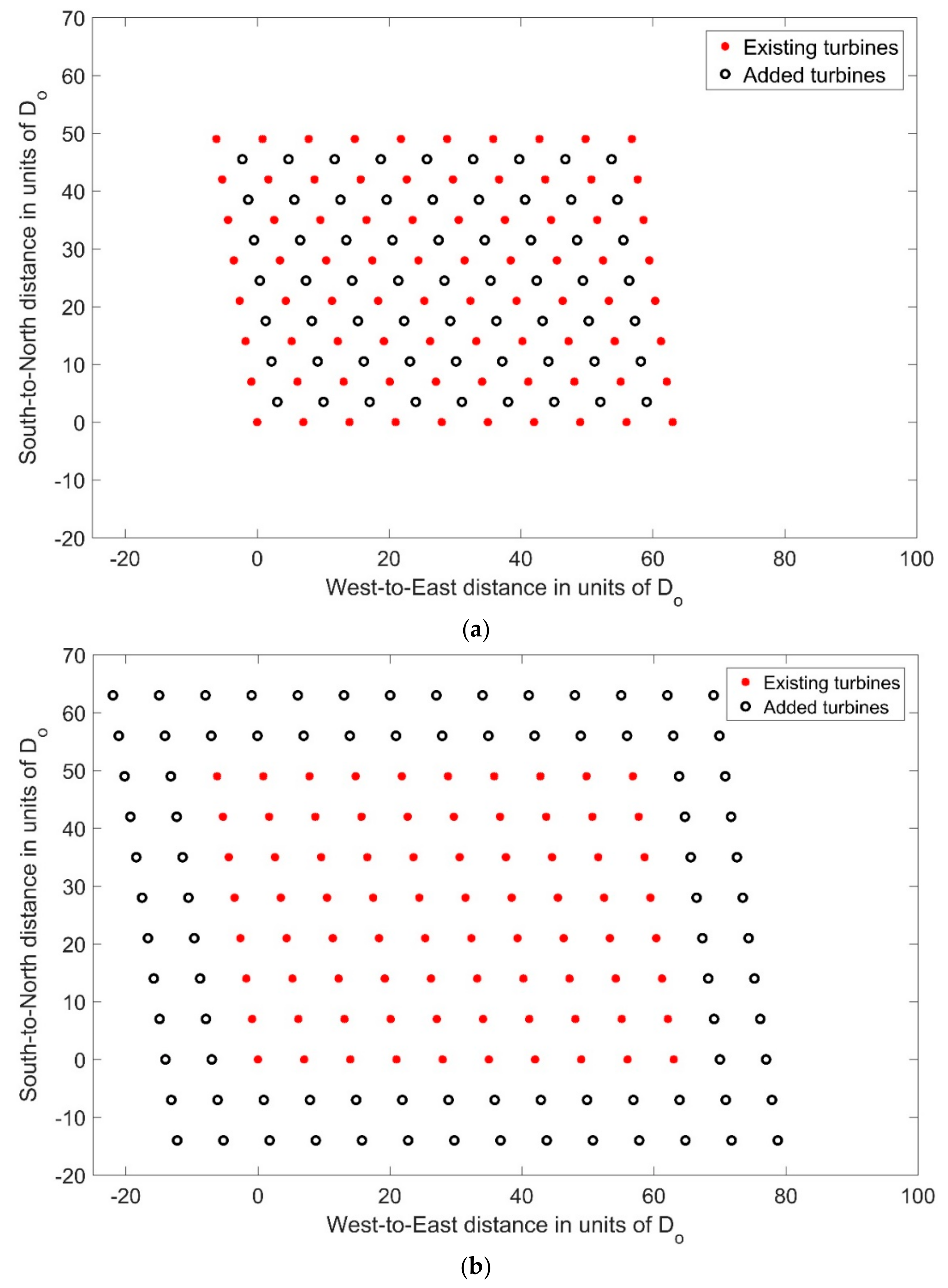
3.1. Proposed Upgraded Layouts

The development of methodologies for multiple turbine wind farm layouts (variable turbine size and/or hub height), e.g., [26,28,29,30,31], allowed the turbine spacing to be reduced to 3.5 D. This recent finding provides compact farm designs with higher AEP, excellent area and height utilization, without severe wake loss, and, hence, lower COE. These results suggest the possibility of installing new turbines within the area of existing farms with relatively large turbine spacing. It is important to state here that the effects of dynamic loading on the turbine blades are not considered in the present work, as is the case of almost all WFLO literature. For comparison, we also considered additional turbines outside the existing wind farm area. Three upgrade layouts were considered: internal grid, external grid, and external unstructured. Figure 3a shows the internal grid upgrade, in which the existing turbines and farm area were kept unchanged by installing new turbines between the existing ones. This maximizes the utilization of the farm space while reducing the added cost due to extra infrastructure. In the external grid upgrade, Figure 3b, the added turbines form four rows and four columns outside the existing area, in order to allow larger turbines to be installed with the least effect on the existing turbines. In Figure 3a,b, the existing turbines are numbered from 1 to 80 (in solid red), while the added turbines are numbered starting from 81 (in hollow black).

The external unstructured upgrade was investigated by considering the same area and the same number of added turbines as the external grid but with an unstructured (non-grid) layout. The minimum turbine proximity was set as 3.5 D_o, where D_o is the diameter of the original turbines (80 m). In all cases, Vestas turbines were considered as this manufacturer’s turbines were used in the original farm. The number of turbines in the original farm is denoted N (N = 80), while M is the number of extra turbines (M = 63 for the internal grid layout and 68 for both external layouts). In all cases, the existing turbines were numbered from 1 to N, while the added turbines from N + 1 to N + M. The vertical coordinate in Figure 3 indicates the North direction and the values in both vertical and horizontal scales are in multiples of D_o.

As shown in Figure 3, the original farm is a parallelogram of base 63 D_o and height 49 D_o which is unchanged in the internal case. However, the total outside area is a parallelogram of base 91 D_o and height 77 D_o. Defining the Area Factor, AF, for the upgraded layout as the farm area divided by the original farm area, gives AF for the three layouts of 1.0, 2.27, and 2.27, respectively.

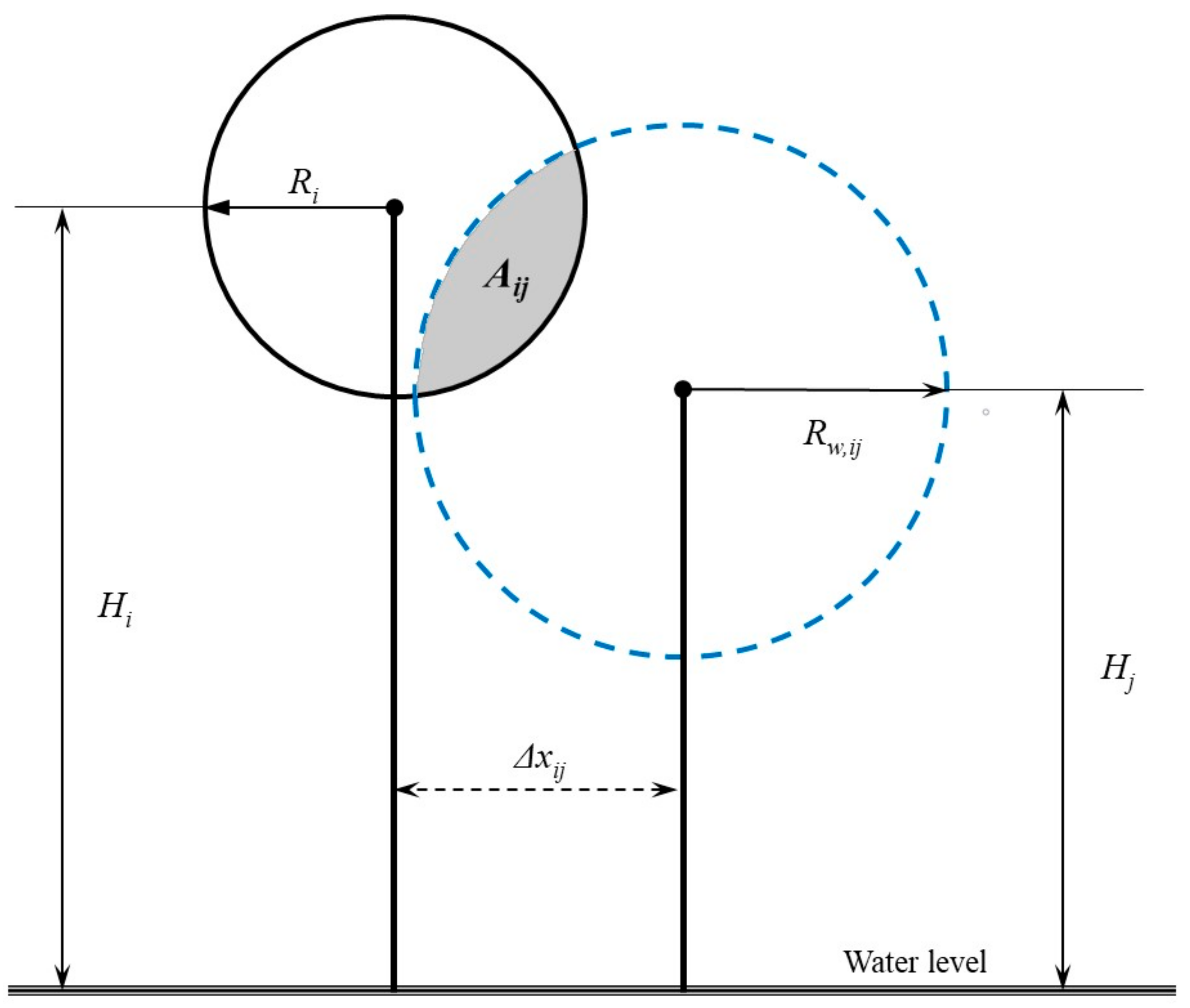
3.2. Wake Model and Interference Calculations

Wake modelling is one of the first and most important steps in WFLO. The availability of the field measurements for some wind farms, especially Horns Rev 1 and Nysted, provided an opportunity to validate the existing wake models and even develop new models. Jensen’s analytical wake model is one of the oldest, simplest, and most accurate in estimating both velocity and power deficits within wind farms, e.g., [22,32,33,34]. Moreover, Reference [26] demonstrated that the model led to accurate estimates of the energy production data for Horns Rev 1 between 2005 and 2015 [14]. Accordingly, the Jensen wake model was implemented in the present wake calculation. Originally proposed by Jensen [35], the model was developed by Katic et al. [36] and Frandsen [37].

In Figure 4, taken from [26], a schematic of the wake interference between an upwind turbine, j, and a downwind one, i, is given. R_w,ij is the radius of the jth turbine’s wake when it reaches the ith turbine, A_ij is the overlap of the jth turbine wake with the downwind turbine rotor, A_i. The Y axis is into the page. The wake calculations were done as follows:

For each wind direction, the coordinates were rotated so that the wind was always in the positive Y-direction. The turbines were then re-numbered in ascending order according to their Y coordinates. For example: the most upwind turbine, which has the least Y-coordinate, was designated 1, while the most downwind one was N + M (the total number of turbines). Accordingly, each turbine, i, in the farm apart from the most upwind one, 2 < i < N, is potentially affected by the wake of every turbine upwind of it: j, 1 < j < i − 1. Defining ∆y_ij = (y_i-−y_j) > 0 and applying the Jensen’s wake model:

$$R_{w,ij}=R_{exp,j}+{\alpha }_j\Delta y_{ij}$$

(1)

$$R_{exp,j}=R_j\sqrt{\frac{1+\sqrt{1-C_{T,j}}}{2\sqrt{1-C_{T,j}}}}$$

(2)

$${\alpha }_j=0.5/ln\left(\frac{H_j}{z_o}\right)$$

(3)

$$\delta U_{ij}=\left\{\frac{1-\sqrt{1-C_{T,j}}}{{\left[1+{\alpha }_j\Delta y_{ij}/R_{exp,j}\right]}^2}\right\}\left(\frac{A_{ij}}{A_i}\right)$$

(4)

$$\delta U_i=\sqrt{{\displaystyle \sum }_{j=1}^{j=i-1}{\left(\delta U_{ij}\right)}^2}$$

(5)

$$U_i= U_{o,i}\left(1-\delta U_i\right)$$

(6)

where C_T is the thrust coefficient for the upwind turbine, δU_ij is the velocity deficit caused by the jth turbine, δU_i is the cumulative velocity deficit caused by all upwind turbines, U_i is the effective wind speed, and U_o,i is the undisturbed wind speed at H_i.

The log law [38] was used to extrapolate wind speed from the reference height in order to estimate the undisturbed wind speed at any height, H_i:

$$U_{o,i}=U_{ref}\left[\frac{\ln \left(H_i/z_o\right)}{\ln \left(H_{ref}/z_o\right)}\right]$$

(7)

The roughness length, z_o, is an essential parameter in wake calculations, on which the vertical wind profile and the wake entrainment greatly depend. The ambient roughness length for offshore farms was taken as 0.0002 m in [22] as is widely accepted for open sea, e.g., [39]. However, the upwind turbines increase the turbulence level within the farm, which in turn increases the effective roughness. As suggested by [40], z_o was taken as 0.05 m “to provide inflow characteristics that are in good agreement with the observed data at Horns Rev” [40], referring to [17,19].

3.3. Commercial Turbines and AEP Calculations

In order to obtain practical upgraded layouts, it was decided to restrict the selection to available models from the same manufacturer as the existing turbines. Accordingly, the selection in the current optimization was among Vestas turbine models. Due to space limitation and to minimize the effect on the existing turbines, the maximum power for the candidate turbines was taken as 3.5 MW and hub height as 140 m. To this end, 19 Vestas turbine models with rated power between 1.8–3.45 MW and diameter between 80–136 m were considered in this study. The turbine rated speed U_R ranged between 10.5–16 m/s. The turbines were sorted and coded in an ascending order according to the rated power and then according to the diameter. The code, rated power, rotor diameter, and rated speed for the 19 turbines are given in

Table 1. Code, rated power, rotor diameter, and rated speed for the turbines included in the selection.

Turbine Code	Rated Power PR (kW)	Rotor Diameter D (m)	Rated Speed UR (m/s)
1	1815	90	13
2	1815	100	11.5
3	2000	80	14
4	2000	90	13
5	2000	100	12
6	2000	110	11
7	2600	100	15
8	3000	90	16
9	3000	112	12
10	3000	126	10.5
11	3075	112	13
12	3300	105	13.5
13	3300	112	12.5
14	3300	117	13
15	3450	105	13.5
16	3450	112	12.5
17	3450	117	11.5
18	3450	126	11.5
19	3450	136	11

.

The manufacturer’s power curves for the 19 turbines were subdivided into four zones separated by cut-in speed, U_in, the rated speed, and the cut-out speed, U_out. The second zone (of a cubic nature) was fitted by a fifth degree polynomial for more accuracy than a cubic fit. The coefficients were used to evaluate the power output from any turbine, i, as function of the effective wind speed, U_i, ahead of its rotor. Accordingly, the individual power, P_i, of the ith turbine based on its type and the effective wind speed, U_i, was evaluated as:

$$P_i=\left\{\begin{array}{cc}0& U_i < U_{in,i}\\ \begin{array}{c}{c}_{i0}+c_{i1}{U}_i+c_{i2}{U}_i{}^2+ c_{i3}{U}_i{}^3+ c_{i4}{U}_i{}^4+ c_{i5}{U}_i{}^5\\ P_{R,i}\end{array}& \begin{array}{c} U_{in,i} \le U_i \le U_{R,i}\\ U_{R,i}<U_i<U_{out,i}\end{array}\\ 0& U_i\le U_{out,i}\end{array}\right\}={\displaystyle \sum }_{k=0}^{k=5}{c}_{ik}{U}_i{}^k$$

(8)

The total farm output power, P_F, for each freestream hub height wind speed, v, at each wind direction, θ, is simply the sum of the individual powers from all turbines:

$$P_F{}_{\left(\theta ,v\right)}={\displaystyle \sum }_{i=1}^{N+M}{P}_i.$$

(9)

The AEP was calculated as:

$$\mathrm{AEP}=8766{\displaystyle \sum }_{\theta =0}^{360}{\displaystyle \sum }_{v=4}^{25}{f}_{\left(\theta ,v\right)}{P}_F{}_{\left(\theta ,v\right)}$$

(10)

where f is the frequency of occurrence of a particular freestream speed at particular direction, Figure 2, and 8766 is the number of hours per year.

3.4. Hub Height Variation

The hub height, H, is one of the most important design parameters for a wind turbine, upon which power and cost greatly depend. In general, higher height means higher wind speed and low wind shear and turbulence levels combined with significant technical and financial difficulties. The optimum value of H for a specific turbine should consider the turbine diameter, rated speed, installation cost, wind resources, site restrictions, etc. Moreover, many recent WFLO studies, e.g., [26,31,41,42], suggest varying H for the turbines within the farm, in order to minimize the wake interference, the installation cost, or a combination of them. In our previous work [26] it was decided to use common H limits (80 m ≤ H ≤ 140 m) for all turbines. However, in the present work, the investigated range of H is widened, and each turbine is given individual H limits according to the turbine diameter. The utilization of the maximum feasible hub height is meant not only to reduce the wake loss, but also to increase the energy production by operating at higher wind speeds and lower turbulence levels. The maximum tip height and the minimum ground clearance are used to determine the individual H range for each turbine, based on its diameter. These two parameters are simply the blade tip height at its highest and lowest positions, respectively. The maximum tip height is set as 230 m for Horns Rev wind farms [43], which is slightly less than the world’s tallest installed wind turbine [44]. On the other hand, the recommended value for the minimum ground clearance ranges from 5 m to 23 m [45]. The proper value depends on the site features: the roughness length for onshore farms and the combination of wave height and tidal range for the offshore ones. Regarding to Horns Rev site, the rare combination of maximum wave height and tidal range is less than 7 m, the mean value is about 3 m [14]. To this end, the maximum tip height and the minimum ground clearance are taken as 200 m and 15 m, respectively. Accordingly, the individual turbine’s H limits can be simply calculated.

3.5. Modified Simple Cost Model

The cost model used in this study is a modified version of the simple model introduced and described in detail in [26]. It was decided to represent all costs in terms of the two design parameters (rated power and hub height). The costs were represented in index form instead of money value and then normalized in order to get qualitative results. The following are the assumptions that led to the cost model used in the present work, supported by references:

• The Total Cost of a wind farm is a combination of the Capital Cost, C_C, and the Operation and Maintenance cost, O&M, C_O&M. It was assumed that, fractionally, C_C = 0.75, while C_O&M = 0.25 [10].
• C_C in turn is subdivided into the total turbine cost, C_turbine = 0.329 C_C, and the remainder, 0.671 C_C, is the Financial and Balance of System costs, C_F&B [46].
• The tower cost for offshore farms, C_tower, was assumed to be 0.1831 C_turbine [46] providing that the turbine is at its minimum H, H_{min, i}. Each 1.0 m increase of H_i over H_{min, i} was assumed to add C_tower/H_{min, i} to the capital cost [26].
• C_F&B depends mainly on the farm area, as the number of turbines is fixed for each layout. Accordingly, the foundation and the other infrastructure costs were assumed fixed for each layout and. In other words, if the turbines were added within the original farm area, the added C_C would comprise only C_turbine while C_F&B was considered unchanged.
• The cost of a 1.0 MW turbine installed at the corresponding H_min, according to its rotor diameter, was taken as the Unit Cost Index, UCI. The corresponding capital and total costs were denoted Capital Cost Index, CCI, and Total Cost Index, TCI, respectively.

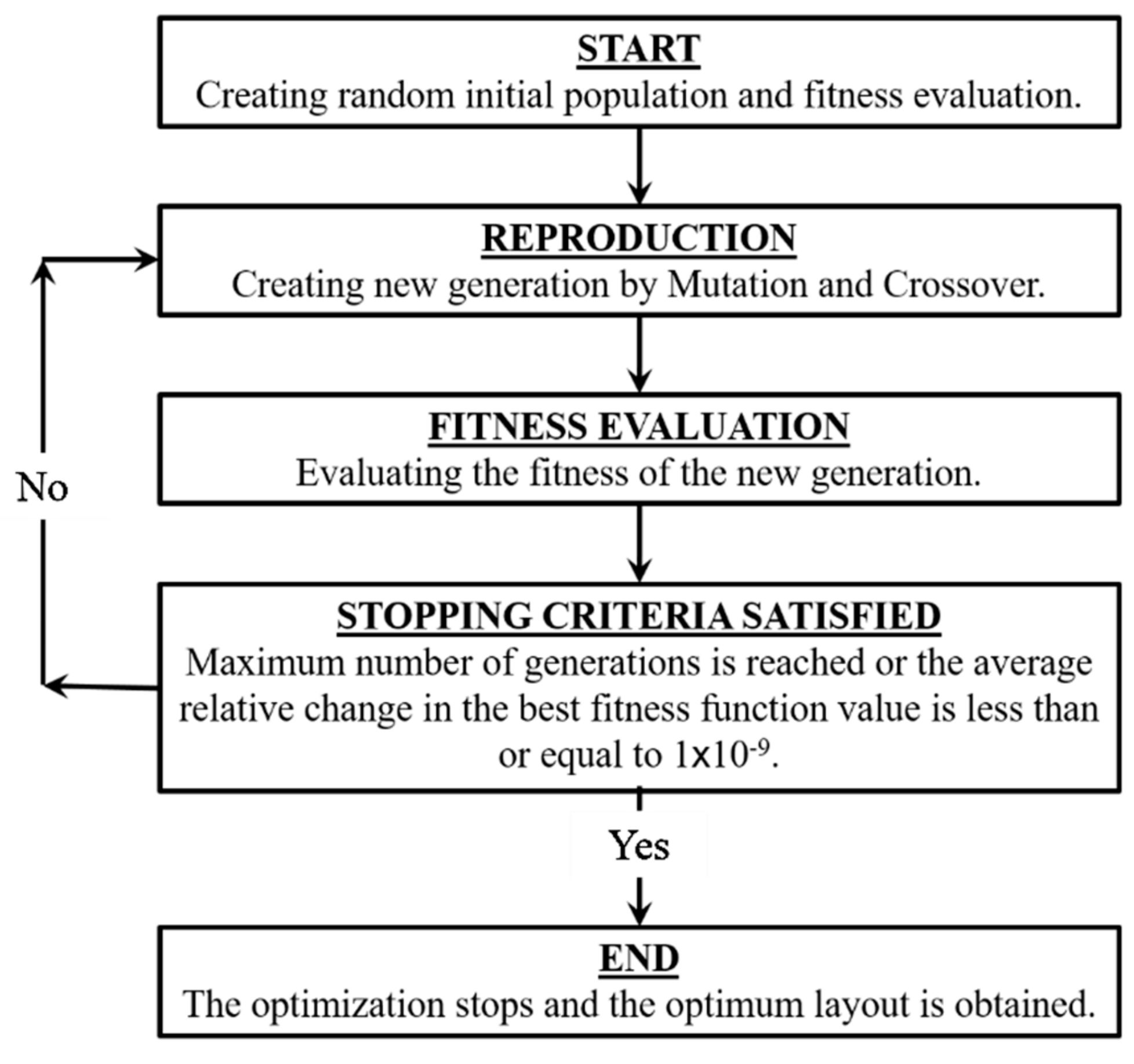
Accordingly, the CCI and TCI for any turbine, i, is expressed as:

$${\mathrm{CCI}}_i=P_{R,i}\left[1+\frac{C_{tower}}{H_{min,i}}\left(H_i-H_{min,i}\right)\right]$$

(11)

and:

$${\mathrm{TCI}}_i=\mathrm{AF}\left[\frac{1}{\left(1-C_{O\&M}\right)\left(1-C_{turbine}\right)}\right]{\mathrm{CCI}}_{\mathrm{i}}.$$

(12)

The added CCI and TCI as a result of the farm upgrade can be expressed as:

$${\mathrm{CCI}}_a={\displaystyle \sum }_{i=N+1}^{N+M}{P}_{R,i}\left[1+\frac{C_{tower}}{H_{min,i}}\left(H_i-H_{min,i}\right)\right]$$

(13)

and:

$${\mathrm{TCI}}_a=\mathrm{AF}\left[\frac{1}{\left(1-C_{O\&M}\right)\left(1-C_{turbine}\right)}\right]{\displaystyle \sum }_{i=N+1}^{N+M}{P}_{R,i}\left[1+\frac{C_{tower}}{H_{min,i}}\left(H_i-H_{min,i}\right)\right]$$

(14)

where AF is the Area Factor, as introduced in Section 3.1.

Based on the above analysis, the TCI for the original farm, TCI_O is

$${\mathrm{TCI}}_O=\frac{1.0}{\left(1-0.25\right)\left(1-0.329\right)}{\displaystyle \sum }_{i=1}^{80}2.0\left[1+\frac{0.06}{55}\left(70-55\right)\right]=323 \mathrm{UCI}$$

(15)

Two useful quantities are defined; the Cost Of Added Energy Index (COAEI) and the Cost Of Total Energy Index (COTEI):

$$\mathrm{COAEI}=\frac{{\mathrm{TCI} }_a}{\mathrm{AEP}- {\mathrm{AEP}}_O }$$

(16)

and:

$$\mathrm{COT}\mathrm{EI}=\frac{{\mathrm{TCI} }_a}{\mathrm{AEP}}$$

(17)

where AEP_O = 715 GW-hr/yr is the estimated AEP for the original farm [26].

3.6. Optimization

Layout optimization for large wind farms with commercial turbine selection is discrete, non-convex, non-linear, and of high dimension. Genetic Algorithms (GAs) are of the most successful optimization methods for such complex optimization problems. The capability of GAs has been proven over years, especially with WFLO, e.g., [47]. On the other hand, GAs are computationally expensive compared with other optimization methods, e.g., [29,47,48], as they require successive random searches. The solution evolves from one generation of a fixed population size (PS) to the next generation. In general, the larger the PS, the wider the search, and the greater the probability of finding the global optima. However, a very large PS requires large execution time without significant improvement on the solution, e.g., [49]. Accordingly, it is very important to select the proper PS in order to increase the probability of finding the global optima while keeping the execution time reasonable, e.g., [49]. Following the majority of the WFLO studies and recommendations found in the literature, GA was used in the present work. Figure 5 shows a flowchart for GA procedure.

In order to investigate the feasibility range, the extreme designs of maximizing the AEP and minimizing the COE were considered, individually. The latter was implemented by two different approaches, as given in Equations (13) and (14). The three objective functions considered in the optimization are shown in

Table 2. Definition of the three objective functions.

ObjFun#	Objective	Equation
ObjFun1	max AEP	(10)
ObjFun2	min COAEI	(16)
ObjFun3	min COTEI	(17)

.

For both internal and external grid layouts, two cases were investigated: single turbine and multiple turbines. In the single turbine cases the optimization was done for each turbine type, individually, with only ObjFun1, and H was the only design variable. On the other hand, for multiple turbines cases, both H and turbine type were the design variables and the three objective functions were considered, individually. However, for the unstructured layout, where the turbine location is variable, only single turbines with ObjFun1 were considered, in order to keep the number of design variables, nvars, reasonable. Moreover, as mentioned in Section 3.1, the unstructured layout was constrained by the minimum turbine proximity, set as 3.5 D_o. The hub height was variable in all cases. As mentioned in Section 3.4, the H variation was set for each turbine based on its diameter. Accordingly, the upper and lower bands for H were not the same for all turbines and the individual height was not included explicitly in the optimization design variables. Instead, a fractional parameter denoted “coefficient of height”, C_H, was an optimization design variable with the same lower and upper bounds (0 and 100, respectively) for all turbines. C_H is defined as:

$$C_H=100\left[\frac{H_i-H_{min,i}}{H_{max,i}-H_{min,i}}\right].$$

(18)

Once C_H is selected (during the optimization) for a particular turbine, i, the corresponding value of H_i is calculated from Equation (18) as:

$$H_i=H_{min,i}+ \frac{C_H}{100}\left[H_{max,i}-H_{min,i}\right].$$

(19)

Table 3. The different cases considered in this paper. The objective functions are listed in Table 2.

Layout		Design Variable(s)	ObjFun#	Number of Variables (nvars)
Internal grid (I)	single turbine	CH	1	M (= 63)
	multiple turbines	code, CH	1, 2, 3	2M (= 126)
External grid (E)	single turbine	CH	1	M (= 88)
	multiple turbines	code, CH	1, 2, 3	2M (= 176)
External unstructured (S)	single turbine	x, y, CH	1	3M (= 264)

summarizes the design variables and the optimization objectives for all cases considered in this paper.

WFLUO is subject to the following constraints, when applicable:

• $1 \le cod{e}_i \le 19, N+1 \le i \le N+M$
• $0 \le C_{H,i }\le 1, N+1 \le i \le N+M$
• The turbines must lie between the extended farm area and the original farm area, as shown in Figure 3.
• $\sqrt{{\left(x_i-x_j\right)}^2+{\left(y_i-y_j\right)}^2} \ge 3.5 D_o, N+1 \le i , j\le N+M, \& i \ne j.$

The first constraint is integer linear, the second and the third constraints are float linear, while the fourth constraint is float nonlinear. In order to accelerate the constraint satisfaction in the unstructured layouts, the external grid layout with C_H = 50 and random turbine selection was set as the initial population.

The trade-off between energy production and cost of energy for the three proposed upgraded layouts was investigated. The selection was among 19 Vestas commercial turbines listed in Table 1. These covered a rated power range of 1.8–3.45 MW and a rotor diameter between 80 and 136 m. MATLAB’s genetic algorithm toolbox [50] was employed for the optimization and the three objective functions in Table 2 were considered individually.

4. Results and Discussion

The results for the three cases are discussed in detail in this section. AEP and the TCI were normalized by the corresponding values for the original farm, AEP_O and TCI_O, respectively. The two normalized quantities were denoted NAEP = AEP / AEP_O and NTCI = TCI / TCI_O. Moreover, the NTCI were divided by the NAEP, to give the Normalized Cost Of Energy Index, NCOEI. The NAEP and NTCI are useful in comparing different layouts and arrangements qualitatively relative to the original farm’s AEP and TCI, respectively. Finally, NCOEI helps in depicting and comparing their feasibility.

As mentioned at the end of Section 2, the wind data was given in 12 directional sectors of 30°. Finer resolutions were tested by the authors and validated against the available farm’s AEP data [16]. Very similar results to the 12-sector division were obtained but with much more computational cost. Figure 6 shows the effect of sector angle, θ, on the estimated AEP and execution time, t, normalized with respect to the corresponding values for 30° sectors. Accordingly, it was decided to use the original wind data with 12 sectors in the present work.

In general, it was found that using a population size double the number of variables (PS = 2 nvars) and evolving for 100 generations achieved satisfactory results. Insignificant improvement was obtained beyond these values with increased computational cost. Figure 7 shows mean and best values for one of the investigated cases over 100 generations for PS = nvars and PS = 2 nvars.

Figure 8 shows the NAEP, NTCI, and NCOEI for the single turbine cases and ObjFun1. Moreover, the probability of selection for C_H values for all single turbine cases is given in Figure 9. In these cases, the M added turbines were assumed identical in type, but different in height. It is important to note here that the discrete points in Figure 8 were connected with dotted line for visual aid only. The major findings are summarized as:

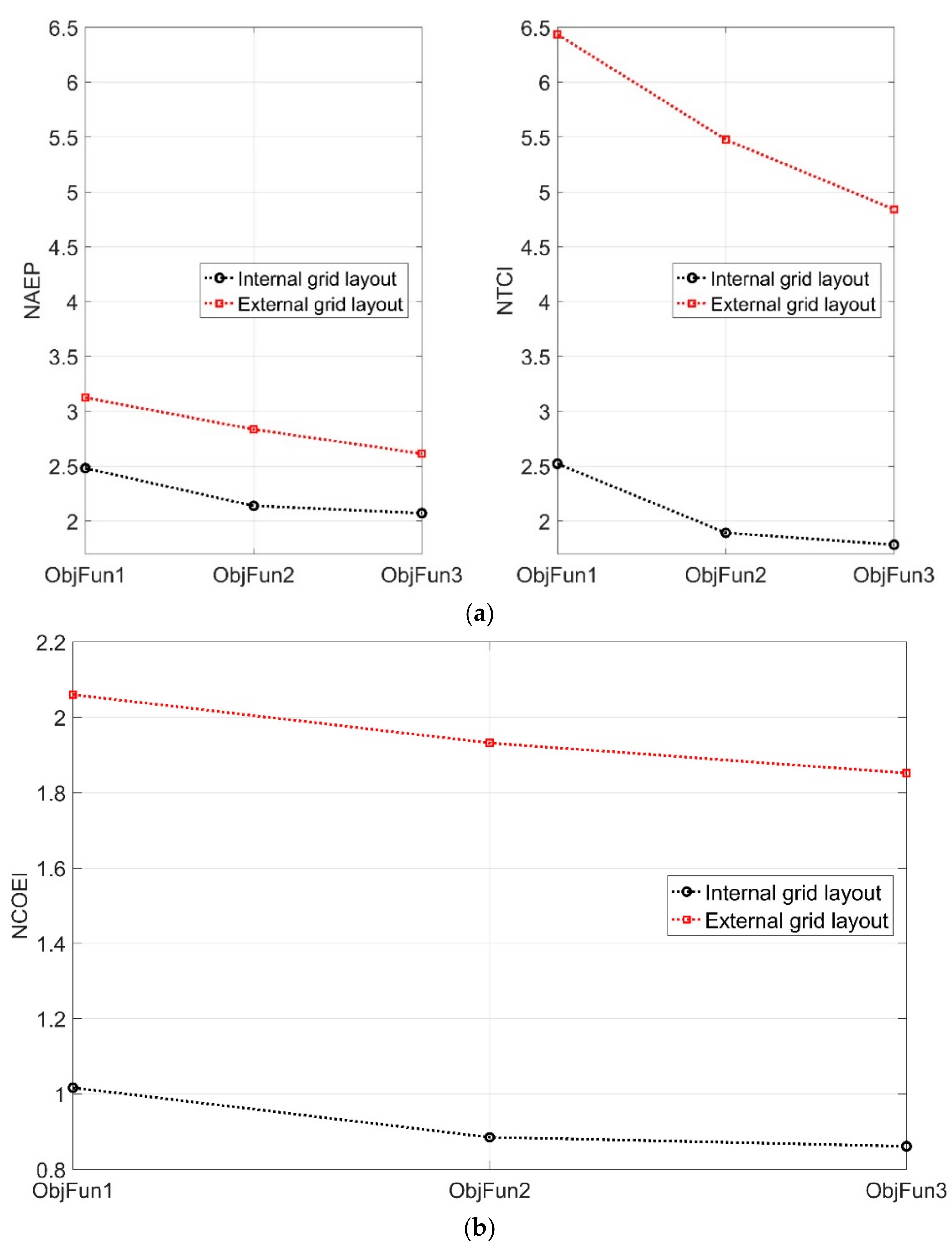
• There is a wide range of feasible optimum upgrades providing a useful trade-off between AEP and COE.
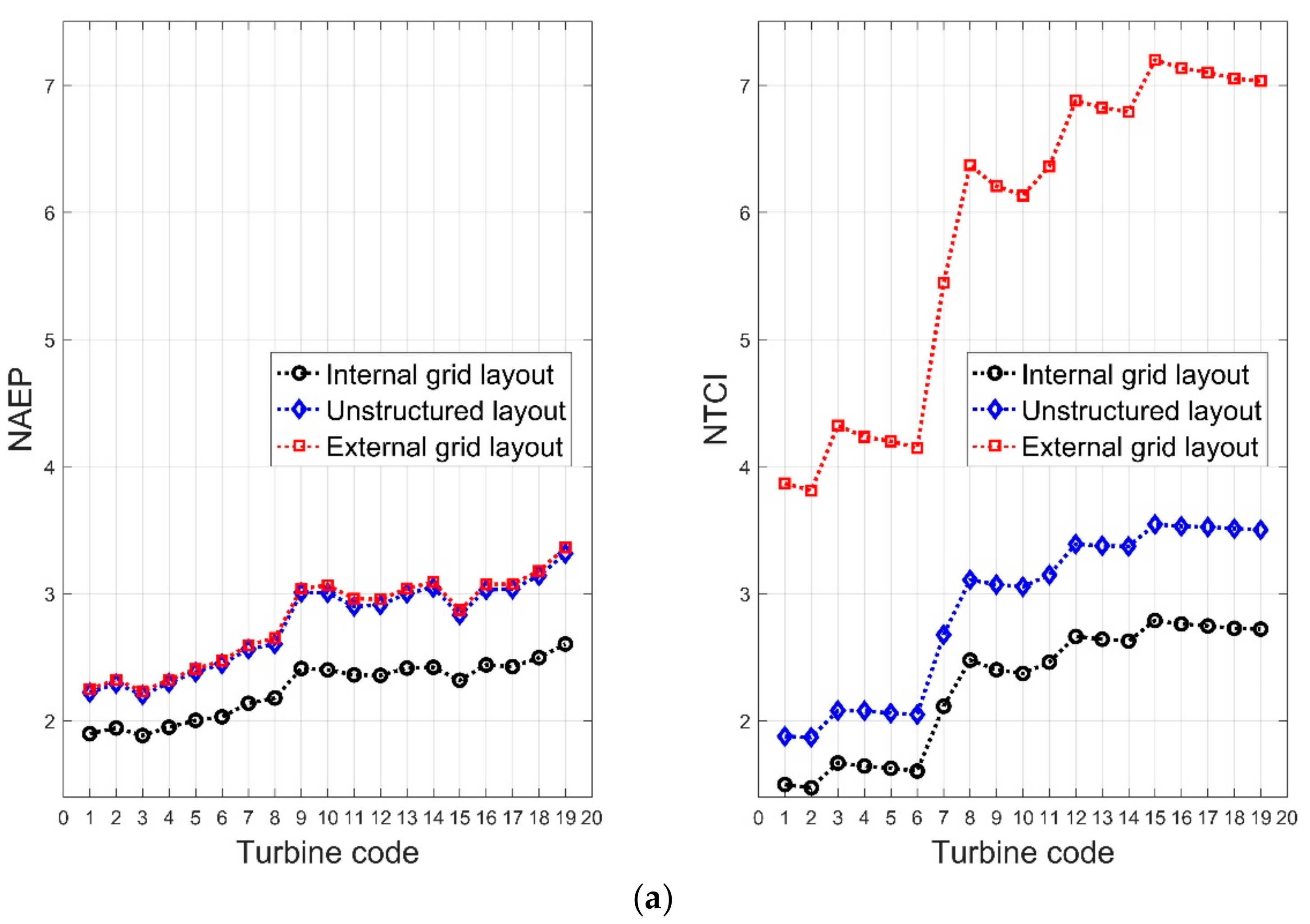
• The single turbine internal layouts produced a range of NAEP from 1.90 to 2.60 with a NTCI from 1.47 to 2.87, depending on the turbine model.
• The single turbine external layouts gave NAEP from 2.23 to 3.36 with a NTCI from 3.81 to 7.20, depending on the turbine model.
• The internal layouts produced cheap additional AEP if small turbines were used. The added AEP increases as the turbine size increases, but at a higher rate in the added cost. The reason is the limited wind resources which causes the increase in AEP to reduce as the turbine size (and hence the cost) increases.
• As expected, the external layouts added more AEP than the internal ones; however, this increase in AEP is accompanied with very high cost as a consequence of adding area to the farm.
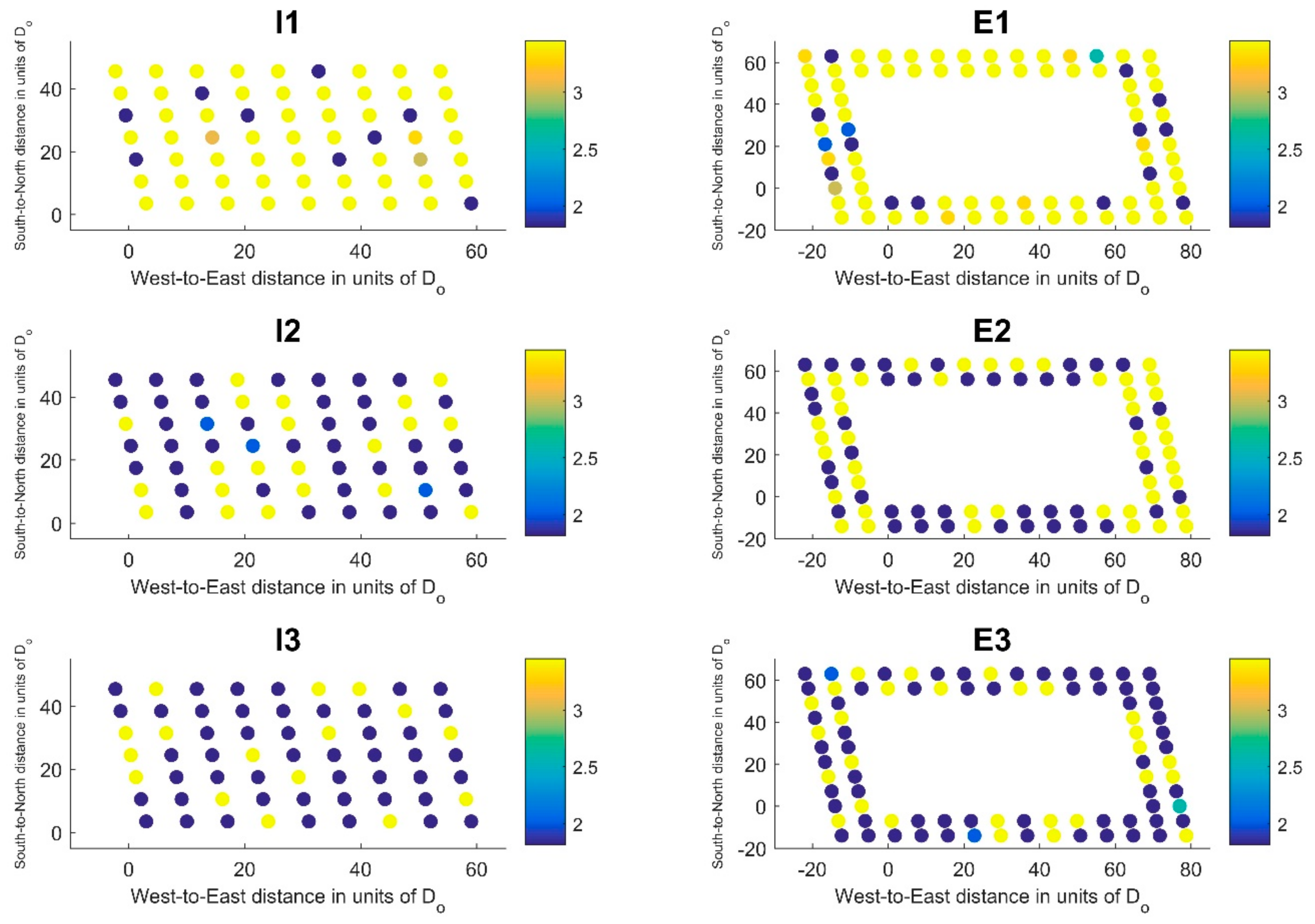
• All layouts have the same trends in AEP and TCI (qualitatively); however, the external grid ones have magnified scales, especially for the cost.
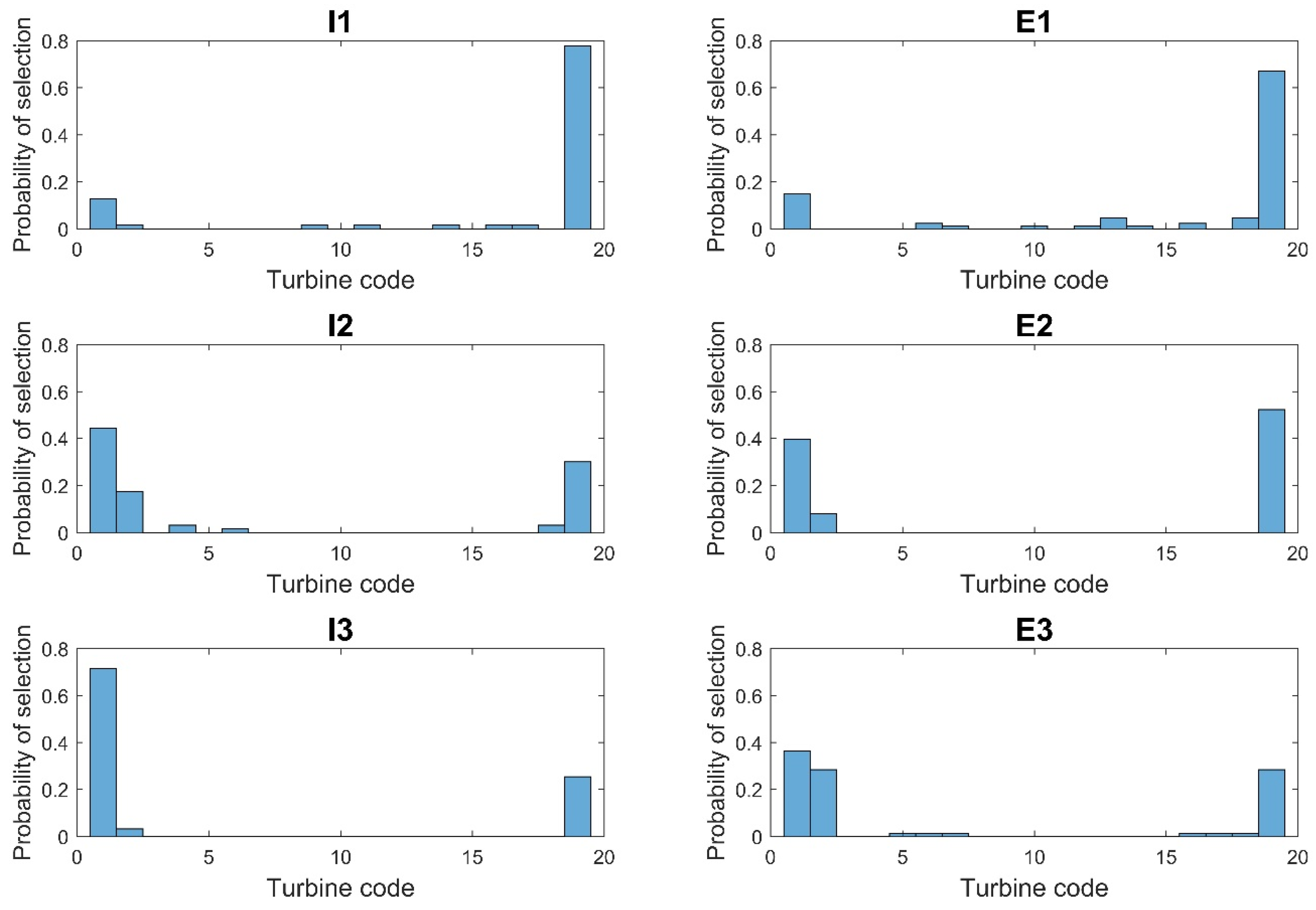
• All layouts confirm the superiority of using turbines with relatively large diameter and relatively low rated speed (turbines number 2, 1, 6, 5, 4, and 3) than the opposite (turbines number 15, 8, 17, 16, and 12). This finding matches that in our previous research [26] and with others in the literature, e.g., [51].
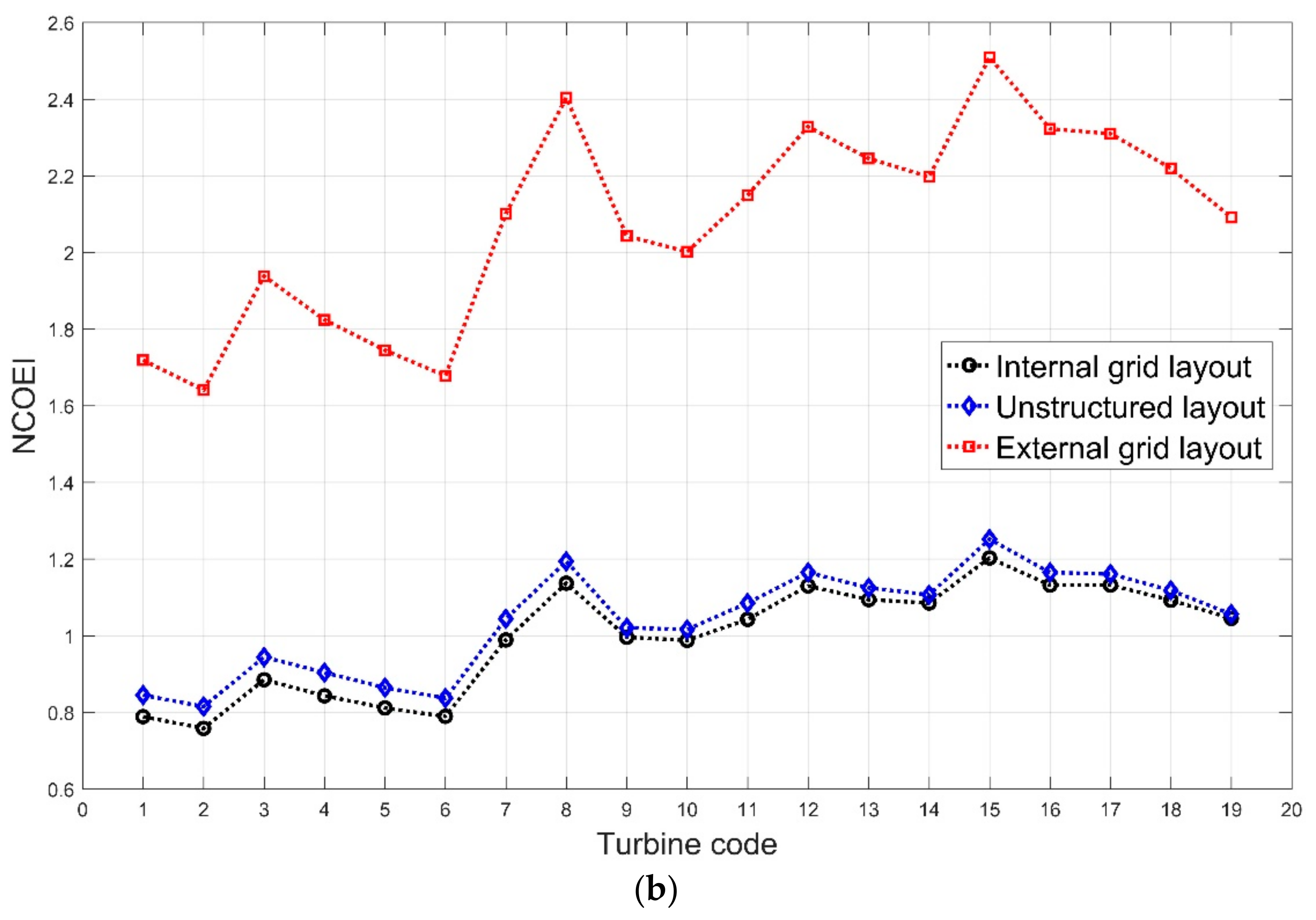
• The NCOEI for the internal layouts are usually close to unity, which means that the added AEP increases comparably to the TCI.
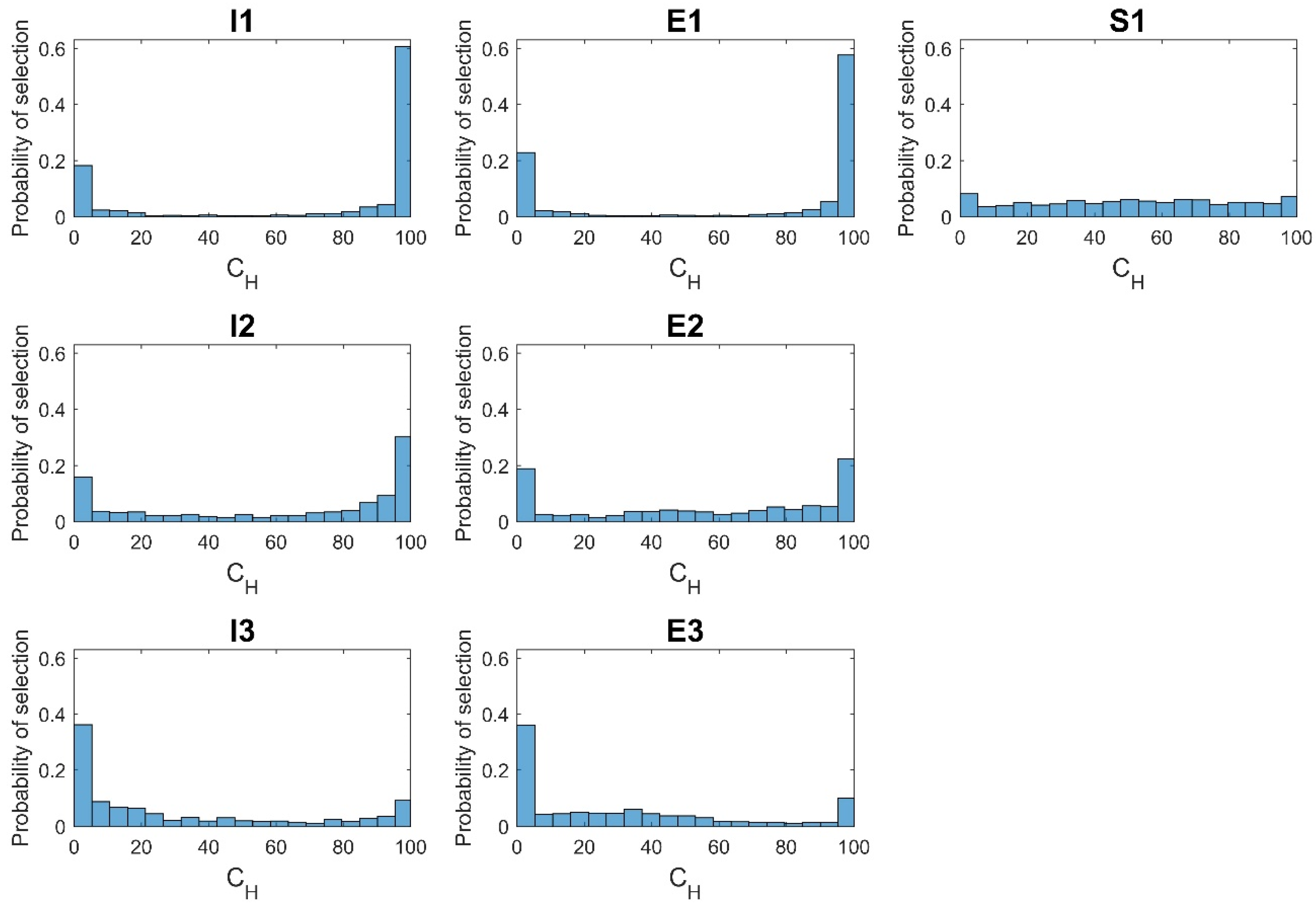
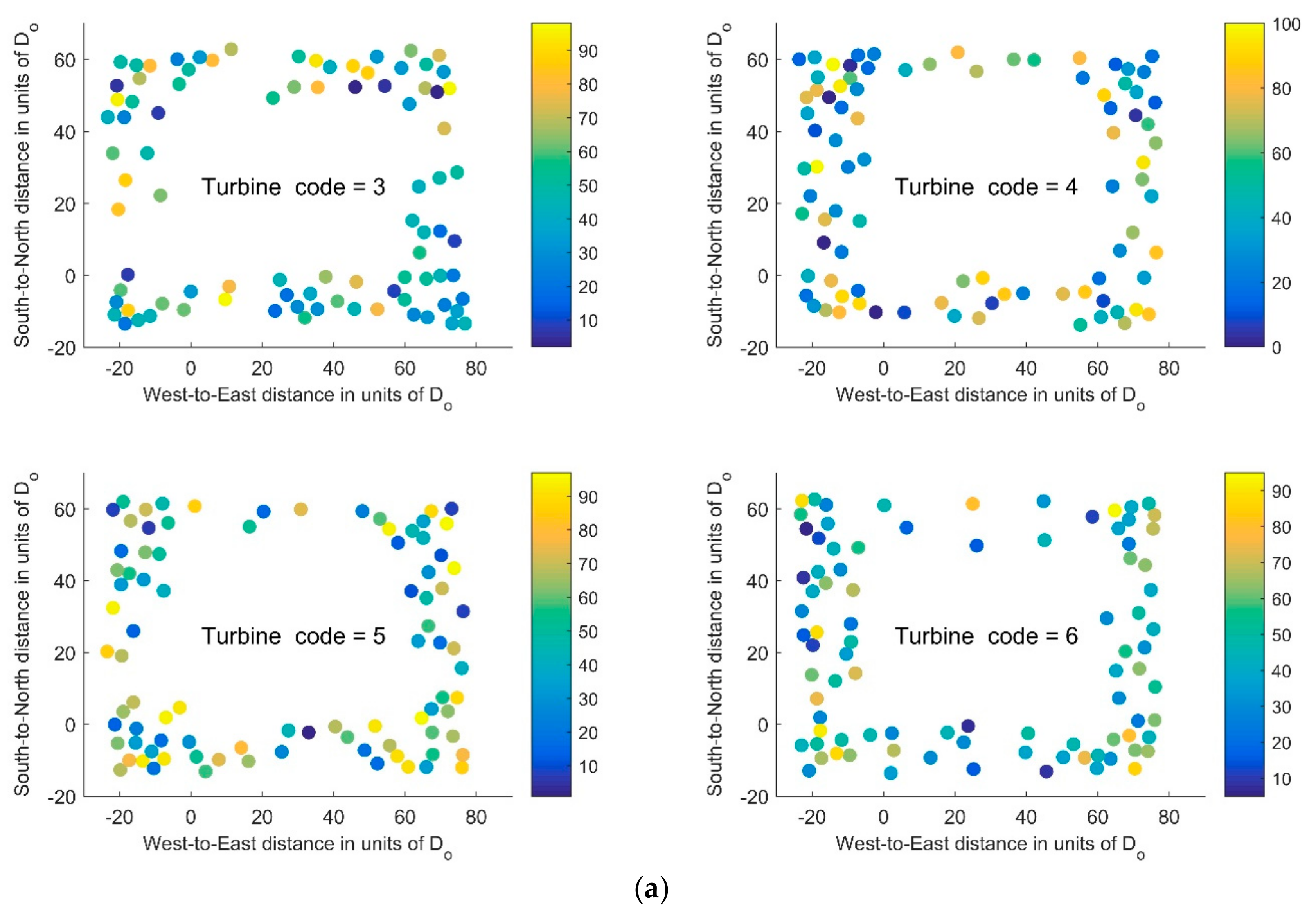
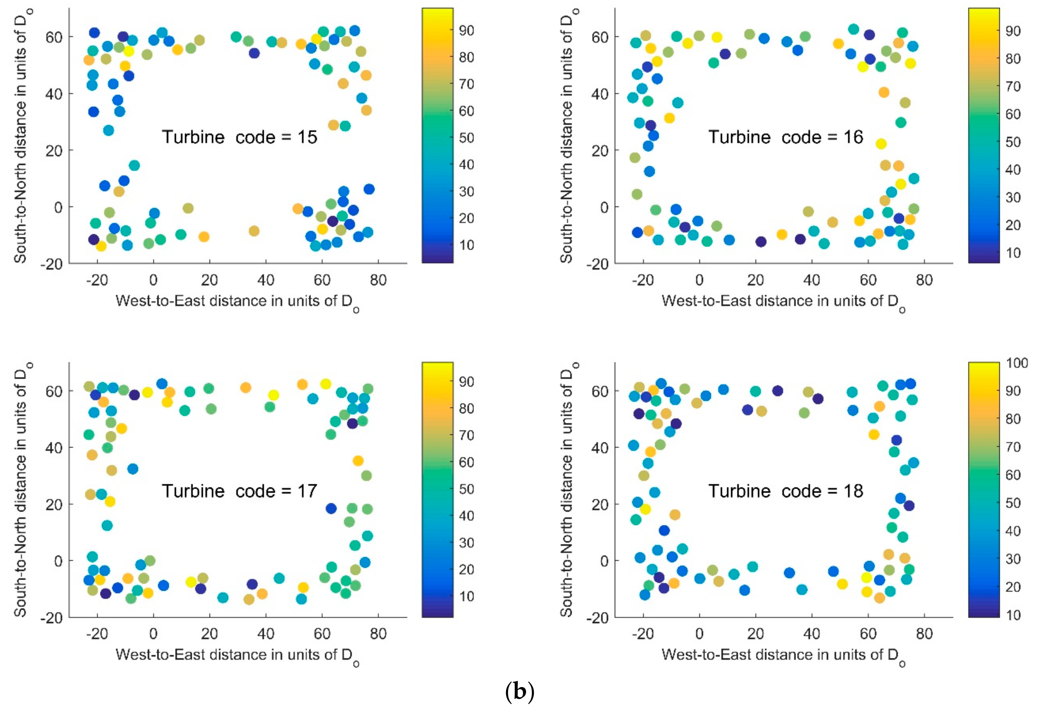
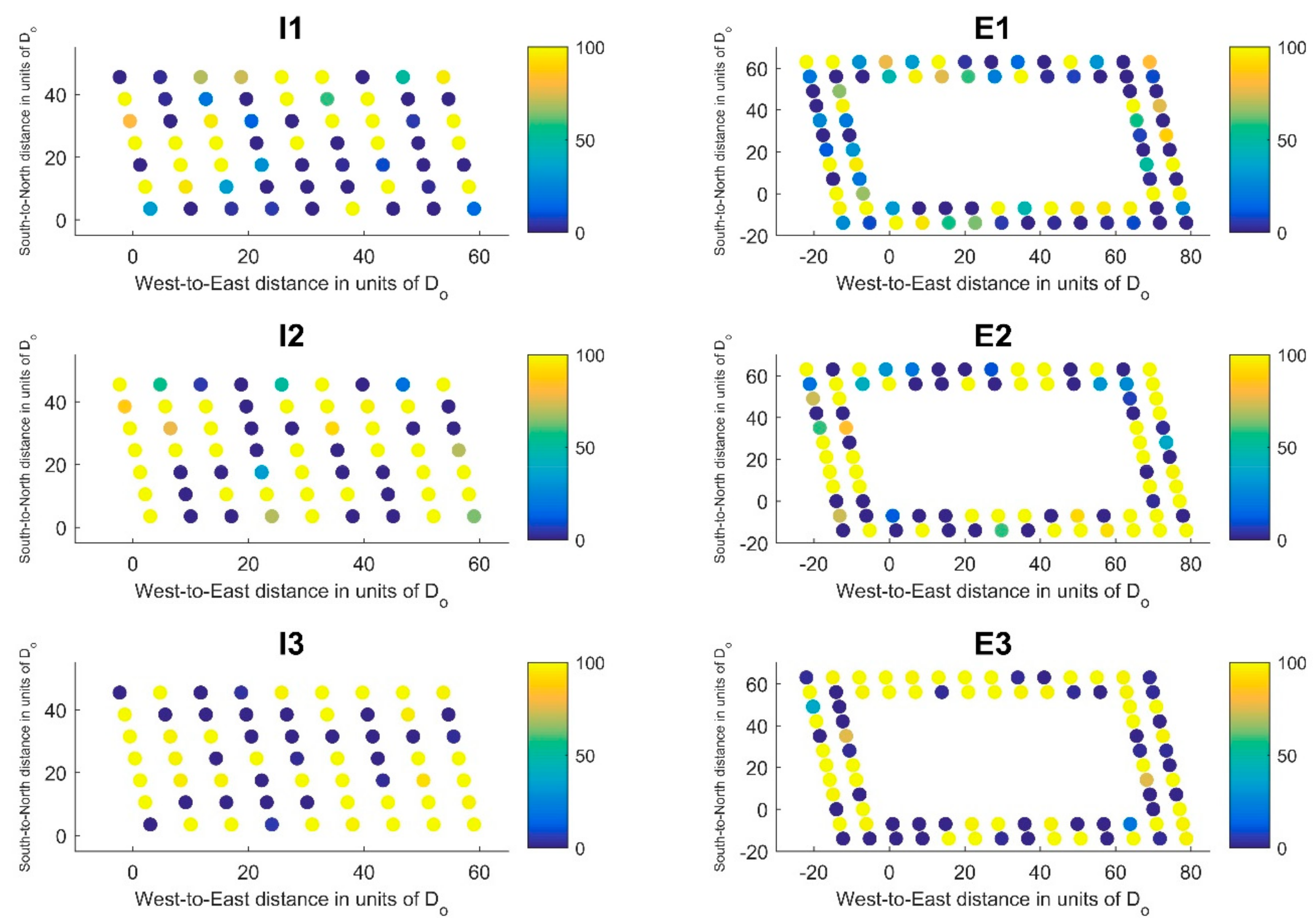
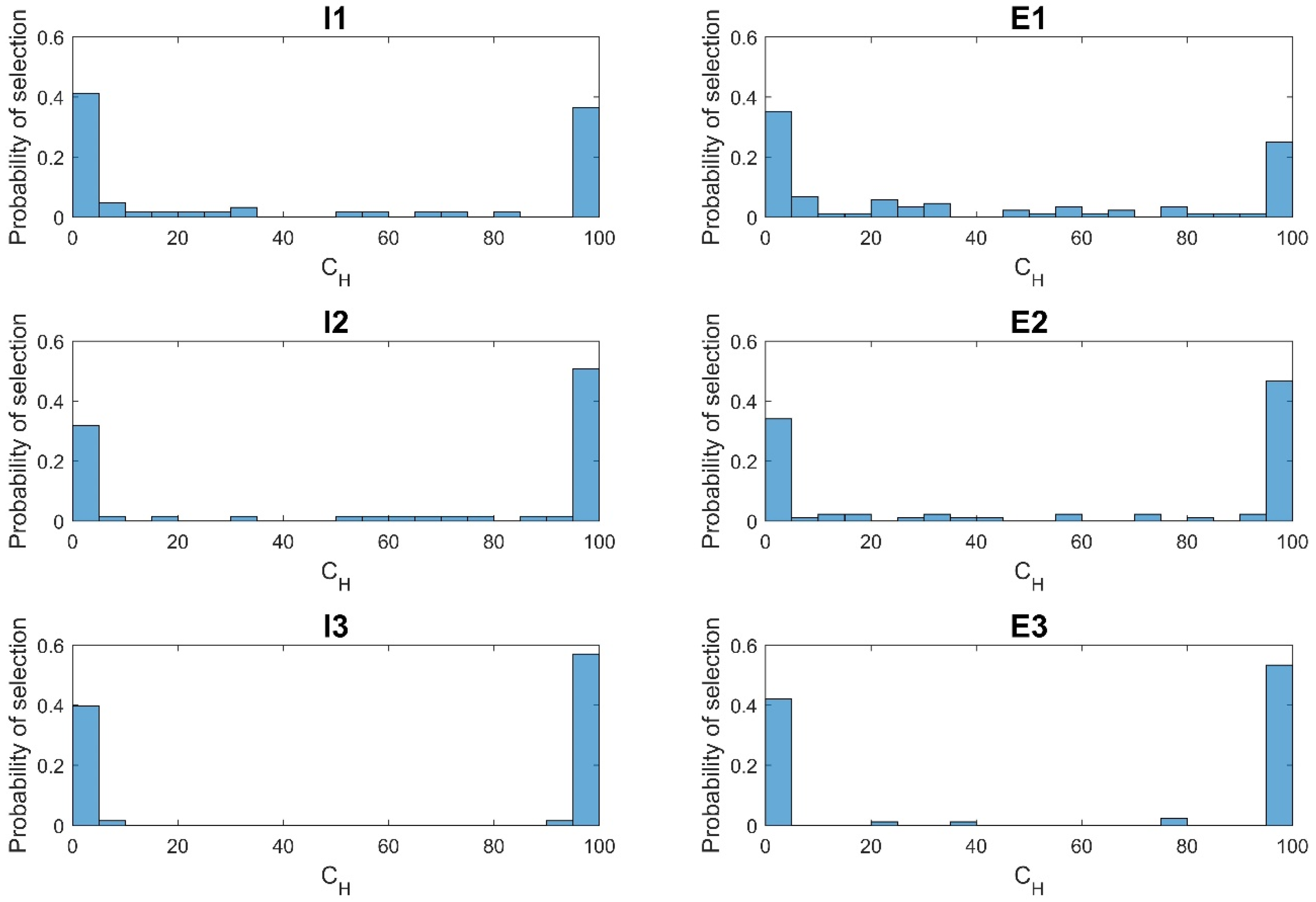
• The unstructured layouts provided almost the same AEP as the external ones with surprisingly much less cost (the NCOEI was close to that of the internal grid layouts). The reason relates to the greater flexibility in locating the turbines which reduces the need for using higher heights to minimize the wake interference. As shown in Figure 9 and Figure 10, a wider range of C_H selections were obtained for unstructured layouts compared with the grid ones. The use of relatively low heights resulted in dramatic decrease in cost.

In Figure 9 and those following, symbols I, E, and S represent the internal grid, external grid, and unstructured layouts, respectively, while the number indicates the ObjFun# as given in Table 2. For example: I2 represents the internal grid layout with ObjFun2. It is clear from Figure 9 that the unstructured layouts have significantly more uniform C_H range compared with the grid ones, which resulted in much less cost, as illustrated in Figure 8. The reason is the flexibility in turbine location which reduces the need for extreme values of H. In the grid layout cases, two clear peaks at C_H = 0 and 100 can be observed. This means that most of the turbines should be installed at the minimum and maximum allowed H in order to reduce the wake interference. It can be also observed that H_max should dominate in maximizing AEP, while this domination should be biased to H_min if the COE minimization is desired.

Figure 10 shows the turbine locations for eight unstructured layouts as a sample of the results, for the sake of brevity. Figure 10a shows the results for turbines 3–6 with P_R = 2 MW, while Figure 10b is for turbines 15–18 with P_R = 3.45 MW. In all cases, the color indicates the C_H values. Two important observations can be drawn:

• The turbines were located more frequently close to the corners. This is understandable because these locations have the least effect on the original turbines.
• In maximizing AEP, more than half the turbines were installed at low and medium heights. This means that properly locating the turbines was much more important than having higher heights in order to maximize the AEP. Accordingly, the cost was reduced dramatically for the unstructured layouts compared with the external grid layouts, Figure 8 and Figure 9.

As the turbine type and turbines locations were fixed in the grid cases, the hub height variation plays the main role in both AEP maximization and COE minimization. For the AEP maximization, the majority of turbines should be installed as high as possible to have the highest possible wind speed. However, the minimum height was required for the rest of turbines, especially in the middle of the farm in the internal layouts, in order to allow wake recovery ahead of the exterior turbines.

For the COE minimizations, heights close to H_min were dominant, and scattered values close to H_max were selected to capture the most power at a few locations and to allow wake recovery for the rest of the turbines at lower heights, which reduced the COE. In general, a wide range of H was used in order to compensate the absence of the turbine selection.

Figure 11 shows the NAEP, NTCI, and NCOEI for the multiple turbine layouts where the M added turbines could be different in both type and height. Again, the dotted lines in Figure 11 were used for visual aid only. The rated power distribution for turbine selection and the corresponding C_H distribution are given in Figure 12 and Figure 13, respectively. The probability of turbine and C_H values selections for all multiple turbines cases are given in Figure 14 and Figure 15, respectively. Again, the external grid layouts give significantly more AEP but with a huge cost (Figure 11) because of the added area (and hence CF&B) compared to the internal layouts. The maximization of AEP (ObjFun1) gave results close to those for the single turbine case of larger size for all layouts. This can be explained by the turbine selection distribution (Figure 12), which shows that maximizing AEP regardless the cost, requires larger turbines as much as possible. The resulting layouts usually have high total cost and COE. Similarly, but at the other extreme, the minimization of COTEI (ObjFun3) gave results close to those for the single turbine case of smaller size for both inside and outside layouts. This can be also explained by the turbine selection distribution (Figure 12) which shows for maximum COE, the selection should be from the smaller turbines in general. Larger turbines should be selected carefully in some places where the increase in power output dominates the corresponding increase in cost. Medium size turbines were rarely used, which means that the proper turbine selection should be, in general, from a few large turbines and a few small ones. The optimization for maximum AEP requires significantly wider range in both turbine size and H. On the other hand, the optimization for minimum COE requires a much smaller range of both turbine size and H.

Finally, a formula was developed to represent NCOEI shown in Figure 8b as function of the turbine’s diameter and rated power. The best fit, was found as:

$$\mathrm{NCOEI}=\frac{ P_R{}^{0.783}}{D^{0.527}}$$

(20)

Equation (20) has a maximum local deviation of 5.5% from the data presented in Figure 8b. This formula could play an important role in comparing two or more turbines from the COE point of view (the smaller the NCOEI the better the turbine to be used). Although the formula represents confirmed trends for P_R and D; however, the specific values are valid only for the case study and the assumptions made throughout the present work. It is clear from Equation (20) that the turbine diameter has an important inverse effect while the rated power is dominant. The effect of the rated speed was found to be negligible, probably because of the relatively high wind speeds considered in the present work. Figure 16 shows the dependence of NCOEI on P_R and D according to Equation (20), within the investigated ranges. Beside the opposite effects of P_R and D on NCOEI, Equation (20), Figure 16 predicts that the use of large diameter is crucial for turbines with high rated power.

5. Conclusions

This paper considers the optimization of wind farm layout upgrade for the first time in the literature as an alternative to repowering a wind farm by replacing the turbines. The proposed upgrade methodology was based on adding new turbines to an existing farm either internal to the farm area or externally. The famous Horns Rev 1 large offshore wind farm was used as a case study. The existing turbines were retained while a similar number of turbines were added in three upgraded layouts: internal grid, external grid, and external unstructured. The selection was from 19 commercial turbines of rated power raged from 1.8 to 3.45 MW. The following are the implications of the findings of this paper:

• Existing middle-aged wind farms can be feasibly upgraded to increase the energy production by adding new turbines, while keeping the cost of energy in reasonable range.
• Wind farm layout upgrade for offshore farms is recommended if it is done within the original farm area and infrastructure. In this case, a significant increase in the energy production can be achieved while keeping the cost of energy in a reasonable range.
• Having a range of commercial turbines for selection as well as allowing variation in height is a powerful tool in the optimization of the wind farm layout upgrade.
• If the added turbines are to be installed outside the original farm area, the unstructured layout has a clear advantage in cost reduction compared to the grid one. It can produce the same output with much less cost.
• By considering more than one objective function, a wide band of feasible optimum layouts is obtained which provide a trade-off between energy production and cost of energy.
• Among commercial turbines having the same rated power, the priority in selection should be biased towards the turbines with larger diameter and lower rated speed.
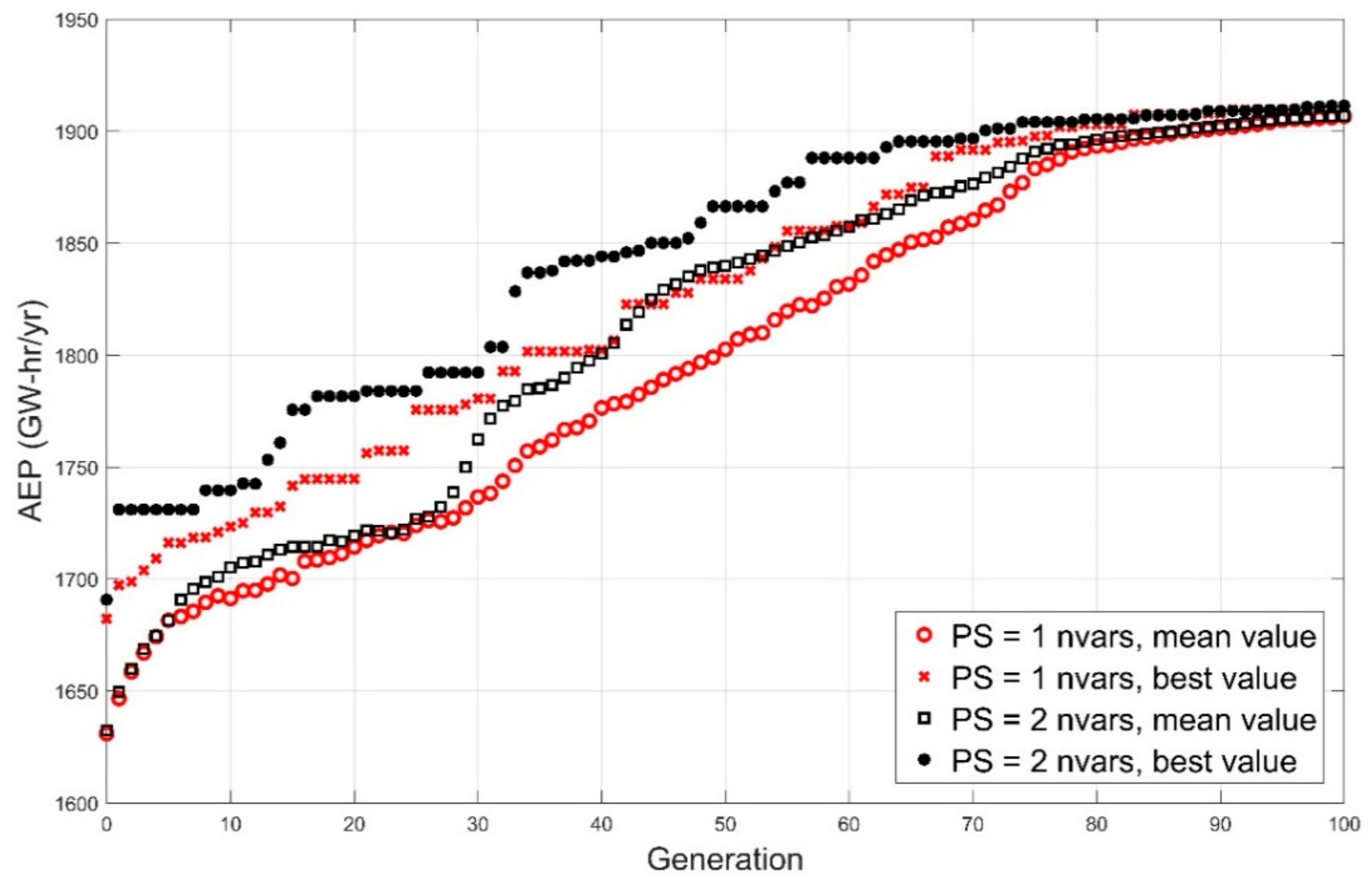
• Using a population size equal to double the number of variables and allowing the evolution over 100 generations is enough to get reasonable results in the present optimization problem.
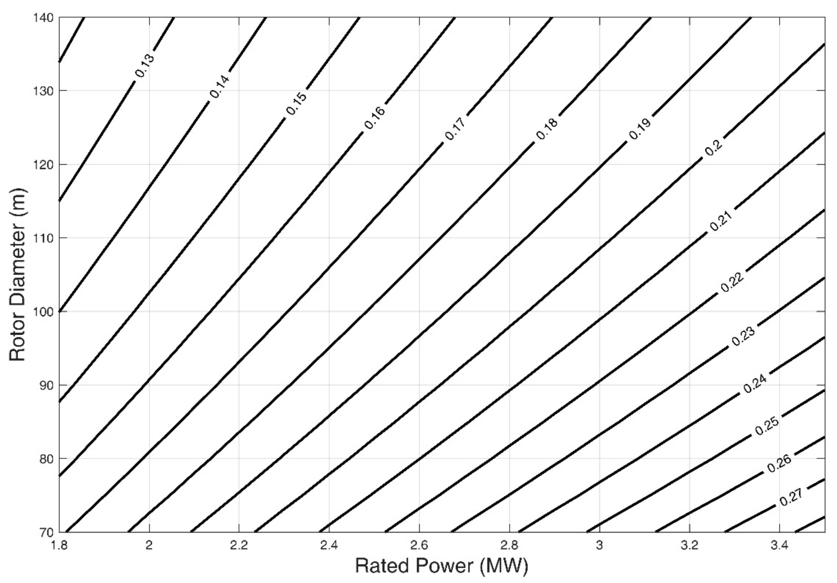
• An approximate formula is given to compare the turbines available for the upgrade, from the cost of energy point of view, based on rated power and diameter.

6. Limitations and Avenues for Future Research

• The cost model was simplified in order to be expressed only in terms of turbines’ rated power and hub height. Consequently, some other factors were not considered, such as: rotor diameter and transportation cost.
• The simple wake models not able to assess the fatigue and other loads associated with multiple turbines, which may well need to be considered in layout optimization.
• The expected effects of wake meandering on wake interference across large farms were not implemented.
• It was assumed that all turbines are available and can be installed at any height within the chosen limits. However, there are associated financial and technical difficulties that were not considered in the selection or in the cost model.

References

1. IRENA. Renewable Power Generation Costs in 2017; International Renewable Energy Agency: Abu Dhabi, UAE, 2018; Available online: https://www.irena.org/-/media/Files/IRENA/Agency/Publication/2018/Jan/IRENA_2017_Power_Costs_2018.pdf (accessed on 3 March 2019).
2. Global Wind Statistics 2017. Global Wind Energy Council (GWEC), February 2018. Available online: http://gwec.net/wp-content/uploads/vip/GWEC_PRstats2017_EN-003_FINAL.pdf (accessed on 3 March 2019).
3. World Energy Perspectives 2016. EXECUTIVE SUMMARY. World Energy Council. Available online: https://www.worldenergy.org/wp-content/uploads/2016/09/Resilience_Managing-cyber-risks_Exec-summary.pdf (accessed on 3 March 2019).
4. The shift Project Data Portal. Available online: http://www.tsp-data-portal.org/all-datasets (accessed on 3 March 2019).
5. BP Statistical Review of World Energy. June 2017. Available online: https://www.bp.com/content/dam/bp-country/de_ch/PDF/bp-statistical-review-of-world-energy-2017-full-report.pdf (accessed on 3 March 2019).
6. Environmental Impacts of Wind Power. Available online: https://www.ucsusa.org/clean-energy/renewable-energy/environmental-impacts-wind-power (accessed on 3 March 2019).
7. Mosetti, G.; Poloni, C.; Diviacco, B. Optimization of wind turbine positioning in large wind farms by means of a genetic algorithm. J. Wind Eng. Ind. Aerodyn. 1994, 51, 105–116. [Google Scholar] [CrossRef]
8. 2014 Wind Technologies Market Report; US Department of Energy, Wind and Water Power Technologies Office: Berkeley, CA, USA, 2015.
9. Lindvig, K. The installation and servicing of offshore wind farms. In European Forum for Renewable Energy Sources; A2SEA A/S: Fredericia, Denmark, 2010. [Google Scholar]
10. Saraswati, N.; Stehly, T.; Dewan, A.; Delmarre, A. Operation and Maintenance Map of U.S. Offshore Wind Farms; ECN-E--17-028. The Netherlands, November 2017. Available online: https://publicaties.ecn.nl/PdfFetch.aspx?nr=ECN-E--17-028 (accessed on 3 March 2019).
11. Wind Farm Lifecycle. Available online: https://canwea.ca/communities/planning-a-wind-farm/ (accessed on 3 March 2019).
12. Hou, P.; Enevoldsen, P.; Hu, W.; Chen, C.; Chen, Z. Offshore wind farm repowering optimization. Appl. Energy 2017, 208, 834–844. [Google Scholar] [CrossRef]
13. Topham, E.; McMillan, D. Sustainable decommissioning of an offshore wind farm. Renew. Energy 2017, 102, 470–480. [Google Scholar] [CrossRef]
14. Sommer, A.; Hansen, K. Wind Resources at Horns Rev; Technical Report, Report No. D-160949; Tech-Wise A/S: Fredericia, Denmark, December 2002; p. 69. [Google Scholar]
15. Jensen, L.; Mørch, C.; Sørensen, P.; Svendsen, K.H. Wake Measurements from the Horns Rev Wind Farm; EWEC: London, UK, 2004; pp. 22–25. [Google Scholar]
16. Overview of the Energy Sector. Available online: https://ens.dk/en/our-services/statistics-data-key-figures-and-energy-maps/overview-energy-sector (accessed on 3 March 2019).
17. Barthelmie, R.; Hansen, K.; Frandsen, S.; Rathmann, O.; Schepers, J.; Schlez, W.; Phillips, J.; Rados, K.; Zervos, A.; Politis, E.; et al. Modelling and measuring flow and wind turbine wakes in large wind farms offshore. Wind Energy 2009, 12, 431–444. [Google Scholar] [CrossRef]
18. Rathmann, O.; Barthelmie, R.; Frandsen, S. Wind turbine wake model for wind farm power production. In Proceedings of the European Wind Energy Conference, Athens, Greece, 27 February–2 March 2006. [Google Scholar]
19. Barthelmie, R.; Pryor, S.; Frandsen, S.; Hansen, K.; Schepers, J.; Rados, K.; Schlez, W.; Neubert, A.; Jensen, L.; Neckelmann, S. Quantifying the impact of wind turbine wakes on power output at offshore wind farms. J. Atmos. Ocean. Technol. 2010, 27, 1302–1317. [Google Scholar] [CrossRef]
20. Frandsen, S.; Barthelmie, R.; Pryor, S.; Rathmann, O.; Larsen, S.; Højstrup, J.; Thøgersen, M. Analytical modelling of wind speed deficit in large offshore wind farms. Wind Energy 2006, 9, 39–53. [Google Scholar] [CrossRef]
21. Frandsen, S.; Rathmann, O.; Barthelmie, R.; Jørgensen, H.; Badger, J.; Hansen, K.; Ott, S.; Rethore, P.; Larsen, S.; Jensen, L. The making of a second-generation wind farm efficiency model complex. Wind Energy 2009, 12, 445–458. [Google Scholar] [CrossRef]
22. Beaucage, P.; Robinson, N.; Brower, M.; Alonge, C. Overview of six commercial and research wake models for large offshore wind farms. In Proceedings of the European Wind Energy Conference & Exhibition; European Wind Energy Association (EWEA 2012), Copenhagen, Denmark, 16–19 April 2012. [Google Scholar]
23. Rivas, R.; Clausen, J.; Hansen, K.; Jensen, L. Solving the turbine positioning problem for large offshore wind farms by simulated annealing. Wind Eng. 2009, 33, 287–297. [Google Scholar] [CrossRef]
24. Vezyris, C. Offshore Wind Farm Optimization Investigation of Unconventional and Random Layouts. Master’s Thesis, TU Delft, Delft, The Netherlands, 2012. [Google Scholar]
25. Park, J.; Law, K. Layout optimization for maximizing wind farm power production using sequential convex programming. Appl. Energy 2015, 151, 320–334. [Google Scholar] [CrossRef]
26. Abdulrahman, M.; Wood, D. Investigating the power-COE trade-off for wind farm layout optimization considering commercial turbine selection and hub height variation. Renew. Energy 2017, 102, 267–516. [Google Scholar] [CrossRef]
27. Feng, J.; Shen, W.Z. Modelling wind for wind farm layout optimization using joint distribution of wind speed and wind direction. Energies 2015, 8, 3075–3092. [Google Scholar] [CrossRef]
28. Herbert-Acero, J.-F.; Franco-Acevedo, J.-R.; Valenzuela-Rendon, M.; Probst-Oleszewski, O. Linear wind farm layout optimization through computational intelligence. In Proceedings of the 8th Mexican International Conference on Artificial Intelligence, Guanajuato, Mexico, 9–13 November 2009; pp. 692–703. [Google Scholar]
29. Tesauro, A.; Réthoré, P.-E.; Larsen, G. State of the art of wind farm optimization. In Proceedings of the European Wind Energy Conference & Exhibition; European Wind Energy Association (EWEA 2012), Copenhagen, Denmark, 16–19 April 2012. [Google Scholar]
30. Chowdhury, S.; Zhang, J.; Messac, A.; Castillo, L. Optimizing the arrangement and the selection of turbines for wind farms subject to varying wind conditions. Renew. Energy 2013, 52, 273–282. [Google Scholar] [CrossRef]
31. Chen, Y.; Li, H.; Jin, K.; Song, Q. Wind farm layout optimization using genetic algorithm with different hub height wind turbines. Energy Convers. Manag. 2013, 70, 56–65. [Google Scholar] [CrossRef]
32. Sørensen, T.; Nielsen, P.; Thøgersen, M.L. Recalibrating Wind Turbine Wake Model Parameters—Validating the Wake Model Performance for Large Offshore Wind Farms; EMD International A/S: Aalborg, Denmark, 2006. [Google Scholar]
33. Sørensen, T.; Thøgersen, M.; Nielsen, P.; Jernesvej, N. Adapting and Calibration of Existing Wake Models to Meet the Conditions Inside Offshore Wind Farms; EMD International A/S: Aalborg, Denmark, 2008. [Google Scholar]
34. Barthelmie, R.; Folkerts, L.; Larsen, G.; Rados, K.; Pryor, S.; Frandsen, S.; Lange, B.; Schepers, G. Comparison of wake model simulations with offshore wind turbine wake profiles measured by SODAR. J. Atmos. Ocean. Technol. 2006, 23, 888–901. [Google Scholar] [CrossRef]
35. Jensen, N. A Note on Wind Generator Interaction. Risø-M-2411; Risø National Laboratory: Roskilde, Denmark, 1983. [Google Scholar]
36. Katic, I.; Hojstrup, J.; Jensen, N. A simple model for cluster efficiency. In Proceedings of the European Wind Energy Association Conference and Exhibition, Rome, Italy, 7–9 October 1986; pp. 407–410. [Google Scholar]
37. Frandsen, S. On the wind speed reduction in the center of large clusters of wind turbines. J. Wind Eng. Ind. Aerodyn. 1992, 39, 251–265. [Google Scholar] [CrossRef]
38. Oke, T.R. Boundary Layer Climates, 2nd ed.; Methuen: London, UK, 1987. [Google Scholar]
39. Wieringa, J. Updating the davenport roughness classification. J. Wind Eng. Ind. Aerodyn. 1992, 41, 357–368. [Google Scholar] [CrossRef]
40. Port-Agel, F.; Wu, Y.; Chen, C. A numerical study of the effects of wind direction on turbine wakes and power losses in a large wind farm. Energies 2013, 6, 5297–5313. [Google Scholar] [CrossRef]
41. Vasel-Be-Hagh, A.; Archer, C. Wind farm hub height optimization. Appl. Energy 2017, 195, 905–921. [Google Scholar] [CrossRef]
42. Chen, K.; Song, M.X.; Zhang, X.; Wang, S.F. Wind turbine layout optimization with multiple hub height wind turbines using greedy algorithm. Renew. Energy 2016, 96, 676–686. [Google Scholar] [CrossRef]
43. Horns Rev 3. Technical Project Description for the Large-Scale Offshore Wind Farm (400 MW) at Horns Rev 3. 43. Document no. 13/93461-2897, 28.04.2014. Energinet/DK: Erritsø, Denmark. Available online: https://ens.dk/sites/ens.dk/files/Vindenergi/horns_rev_3_offshore_technical_project_description_28.04.201.pdf (accessed on 3 March 2019).
44. World’s Tallest Wind Turbines Built in Germany. Available online: https://electrek.co/2017/11/02/worlds-tallest-wind-turbine-built-in-germany/ (accessed on 3 March 2019).
45. Oteri, F. An Overview of Existing Wind Energy Ordinances; National Renewable Energy Laboratory Technical Report, NREL/TP-500-44439; National Renewable Energy Laboratory: Lakewood, CO, USA, 2008. [Google Scholar]
46. Moné, C.; Stehly, T.; Maples, B.; Settle, E. 2014 Cost of Wind Energy Review; National Renewable Energy Laboratory (NREL): Lakewood, CO, USA, 2015. [Google Scholar]
47. Samorani, M. The Wind Farm Layout Optimization Problem; Technical Report; Leeds School of Business, University of Colorado: Boulder, CO, USA, 2010. [Google Scholar]
48. Khan, S.; Rehman, S. Iterative non-deterministic algorithms in on-shore wind farm design: A brief survey. Renew. Sustain. Energy Rev. 2013, 19, 370–384. [Google Scholar] [CrossRef]
49. Roeva, O.; Fidanova, S.; Paprzycki, M. Influence of the population size on the genetic algorithm performance in case of cultivation process modelling. In Proceedings of the 2013 Federated Conference on Computer Science and Information Systems, Kraków, Poland, 8–11 September 2013; pp. 371–376. [Google Scholar]
50. © 1994-2019 The MathWorks, Inc. Available online: https://www.mathworks.com/help/gads/genetic-algorithm.html (accessed on 3 March 2019).
51. Rehman, S.; Khan, S.A. Fuzzy logic based multi-criteria wind turbine selection strategy—A case study of Qassim, Saudi Arabia. Energies 2016, 9, 872. [Google Scholar] [CrossRef]
Figure 1. The percentage global cumulative installed wind capacity, relative to 2017, adapted from Reference [2].
Energies 12 02465 g001
Figure 2. Contours of frequency of occurrence, f, of wind speed and direction at hub height for Horns Rev 1, adapted from [27].
Energies 12 02465 g002
Figure 3. Two proposed upgrade layouts for Horns Rev 1 wind farm. (a) Internal grid; (b) External grid. The vertical coordinate indicates the north.
Energies 12 02465 g003
Figure 4. A front view (parallel to wind direction) illustrates the overlap of an upwind turbine wake (the dashed circle) with a downwind turbine rotor (the solid circle) [26].
Energies 12 02465 g004
Figure 5. Flowchart for genetic algorithm.
Energies 12 02465 g005
Figure 6. Effect of sector angle on the estimated AEP and execution time, t, normalized with respect to the corresponding values for 30° sector.
Energies 12 02465 g006
Figure 7. Convergence history for one of the investigated cases over 100 generations for PS = 1 nvars and PS = 2 nvars.
Energies 12 02465 g007
Figure 8. Results for single turbine cases and ObjFun1 for all layouts. (a) Normalized annual energy production and normalized total cost index; (b) Normalized cost of energy index.
Energies 12 02465 g008aEnergies 12 02465 g008b
Figure 9. Probability of selection for CH values for all single turbine cases.
Energies 12 02465 g009
Figure 10. Turbine locations and CH values for selected unstructured cases. (a) Turbines 3–6 with PR = 2 MW; (b) Turbines 15–18 with PR = 3.45 MW.
Energies 12 02465 g010aEnergies 12 02465 g010b
Figure 11. Results for multiple turbines grid layouts. (a) Normalized annual energy production and normalized total cost index; (b) Normalized cost of energy index.
Energies 12 02465 g011
Figure 12. Rated power distribution in MW for the selected turbines for multiple turbines grid layouts.
Energies 12 02465 g012
Figure 13. Coefficient of height, CH, distribution for multiple turbines grid layouts.
Energies 12 02465 g013
Figure 14. Probability of turbine selection for multiple turbines grid layouts.
Energies 12 02465 g014
Figure 15. Probability of selection for CH values for multiple turbines grid layouts.
Energies 12 02465 g015
Figure 16. NCOE dependence on PR and D.
Energies 12 02465 g016