A Deep-Sea Pipeline Skin Effect Electric Heat Tracing System

Abstract

In order to ensure deep-water flowline safety, this paper combined the axial temperature distribution model of the submarine pipeline and the distributed parameter circuit model of the skin effect electric heat tracing system; such work is conducive to proving that the heating effect of the skin effect electric heat tracing system depends on the distributed circuit parameters and power frequency of the system. Due to the complexity of the power supply device, the frequency cannot be increased indefinitely. Therefore, for the case that the input of the skin electric heat tracing system is constrained, a generalized predictive control algorithm introducing the input softening factor is proposed, and the constrained generalized predictive control strategy is applied to the electric heating temperature control system of the submarine oil pipeline. Simulation results demonstrated that the control quantity of the skin effect electric heat tracing system is effectively controlled within a constraint range, and also the values of heating power and power frequency are obtained by theoretical calculations rather than empirical estimations. Moreover, compared with the conventional control algorithm, the proposed constrained generalized predictive algorithm unfolds more significant dynamic response and better adaptive adjustment ability, which verifies the feasibility of the proposed control strategy.

1. Introduction

In order to prevent crude oil from solidifying and waxing in submarine pipelines, active heating of submarine pipelines, reducing heat loss of pipelines and reducing temperature drop along the way have become the key to efficient and safe transportation of offshore crude oil pipelines. The electric heat tracing technology has been considered to be one of the active heating methods for the deep-water submarine pipeline with the highest heating efficiency [1,2,3]. The skin effect electric heat tracing for metal pipe heating can be favored for providing heat tracing for long-distance pipelines [4]. In 2009, the first skin-effect electric heat tracing system submarine pipeline was put into use in the Bohai Sea area, China, with a heating length of up to 11 km [5]. To ensure the efficient transportation of crude oil in the pipeline, it is necessary to determine the heating power of the skin effect electric heat tracing system according to factors such as the nature of the crude oil, the ambient temperature and the characteristics of the pipeline [6]. However, there is currently no quantitative study on the calculation of system equivalent impedance with frequency in the skin effect electric heat tracing system. Therefore, the heating power and frequency of the skin electric heating system can only be estimated according to the actual engineering experience, and the existing thermal management strategies have the disadvantages of low heating energy efficiency, slow adjustment speed, and single-temperature control algorithm.

In view of the shortcomings in the above research, many scholars have carried out a series of studies on electric heating systems. One of the most important parameters for the circuit theory is the impedance, which is frequency dependent and can be found from the general equations [7]. For design and rating of the DEH system, Lervik et al. proposed the supply current, the power loss (heat generation) in the pipeline and the total system impedance are the governing parameters [8]. Ahlen and Torkildsen [9] proposed the induction through thermal insulation (ITTI) system, and analyzed the influencing factors of heating power for the system. Based on this, an equivalent circuit model for heating cables was established. However, the exact expression for solving the equivalent impedance is not given in the text, which leads to the lack of clear heating power. Reference [10] analyzed the temperature distribution law of heavy oil wells, established a circuit model for electric heating special cable and gave the calculation formula of heating power of each cable. Unfortunately, for a given cable, the distribution parameters are not considered to change with frequency, so there is a bias in the calculation of the heating power. Fang et al. also analyzed the vertical temperature distribution of heavy oil wells and established a circuit model for special heating cables; the relationship between the equivalent impedance and frequency of the heat-resistant cable under certain structure and material is obtained by fitting, so that the cable heating power is more accurate [11]. In [12], the heat generation in the pipeline depends on several parameters, like the magnetic properties of the pipeline and the pipeline resistivity. These parameters are greatly affected by the power frequency of the supply current. A higher power frequency increases the heat efficiency of the pipeline current. In addition, the key to the research of electric heating technology of oil pipeline is the calculation of pipeline temperature field and heating power.

For this reason, this paper starts with the axial temperature distribution model of the submarine pipeline and the equivalent circuit model of the distribution parameter of the skin effect electric heat tracing system. Using the combination of circuit principle and electromagnetic theory, the impedance value of the distributed parameter model with frequency is obtained, and the influence of frequency on heating efficiency is discussed. Then combined with the axial temperature distribution model of the submarine pipeline and the power distribution of the heating element, the actual temperature distribution of the submarine pipeline is obtained, which indicates that the heating effect of the skin effect electric heat tracing system depends on the distributed circuit parameters and current frequency of the system. However, the current frequency is not fixed as high as possible, but should be adjusted according to change in load temperature. So far, there is very little research about establishing an effective mathematical model for the skin effect electric heat tracing system and applying advanced control strategies to it. This is because the skin effect electric heating system is not easy to measure accurate data in an industrial environment and establish an accurate mathematical model. Even if a mathematical model of the system is established, the optimal control obtained cannot achieve the optimal control effect because the parameters are slowly time-varying during the running process. Researchers have constructed a first-order inertia delay link model for the load model of the skin effect electric tracing system [13]. However, the skin effect electric tracing system is a typical system of thermal system. It is only characterized by a single first-order model and controlled by traditional control algorithms. It is difficult to meet the needs of multi-variable conditions. In Reference [14], the mechanism of the skin effect electric heat tracing system is introduced, and the intermediate variable is also introduced to establish the Hammerstein model. Therefore, the relationship between the power frequency and the heating temperature of the skin effect electric heat tracing system is established, and the power frequency is optimized by the generalized predictive control theory. Unfortunately, the physical constraint problem was neglected. Once the input signal of the actuator exceeds the limit, the control effect will not be implemented, and the meaning of optimization will be lost [15]; the system heating efficiency increases significantly with increasing current frequency, but the complexity of the power supply design limits the unlimited increase in frequency. Considering input constraints in generalized predictive control complicates the problem of rolling optimization for solving control quantities, usually requiring a constrained quadratic programming or non-convex programming problem. A lot of studies have been done on this problem. Demircioglu [16] transformed the constrained optimization problem into a quadratic programming problem, but the iterative solution to the quadratic programming requires a large amount of computation, the objective function constraint is negligible, and the general solution is a locally optimal solution. The genetic algorithm can deal with the constrained optimization problem and obtain the global optimal solution. Some researchers have used the genetic algorithm to solve the objective function of generalized predictive control under the constraint condition, but the genetic algorithm requires binary coding, the programming is complex and the computational cost is large [17,18]. To improve the performance and application range of generalized predictive control, it is necessary to find an effective method to solve the optimization problem. The particle swarm optimization algorithm is easy to understand, easy to implement, and the objective function constraint does not require differentiability. The particle swarm optimization algorithm to solve the constraint problem of generalized predictive control was introduced in References [19,20]. It can be seen that the generalized predictive control with constraints by nonlinear search has become more and more mature in theory. However, with the increase of the number of constraints, the calculation amount increases exponentially. Therefore, it is difficult to popularize and apply the nonlinear programming optimization algorithm in actual control. In Reference [21], the author proposed a new generalized predictive control algorithm with input constraints, adding the concept of input gentle factor, unifying the input constraints and incremental constraints, and simplifying the performance indicators to solve the problem of single-variable system input constraints. Su also introduced the input gentle factor and retained the integrity of the performance indicators, solving the problem of input constraints of multivariable nonlinear systems [22]. All of the above methods avoid the nonlinear programming problem of nonlinear programming, and do not have to solve the Diophantine equation, which greatly reduces the amount of calculation. Therefore, the author proposes a generalized predictive control based on constraints on this basis to achieve temperature control of the skin effect electric tracing system.

In this paper, the heat transfer tube and heating cable of the skin effect electric heat tracing system are regarded as a whole, and the distributed parameter circuit model is established. Furthermore, the equivalent impedance value of the frequency change is analyzed to obtain the heating power of the system, which avoids the blindness of the design of the intermediate frequency heating power supply. In addition, the generalized predictive control of the skin electric heat tracing system based on the Hammerstein model is further optimized, so that the designed controller can meet the production requirements under certain limits and work properly under conditions closer to the actual production conditions.

2. System Model

2.1. Axial Temperature Distribution Model

At a water depth of about 350 m, there is a constant temperature layer [23]. As the depth increases, the water temperature slowly decreases, and the water temperature drops by 1 K to 2 K for every 1000 m of water. According to Reference [24], when the water depth in the South China Sea is increased from 350 m to 500 m, the temperature change is not too large. Assuming that the submarine pipeline is laid in the deep water, the temperature gradient can be ignored. For the convenience of analysis, a section of finite element dl can be taken from a pipeline. The temperature of the oil changes to dT through the dl section, and the heat balance equation on the dl section is established during steady-state heat transfer:

$$\mathrm{d}{Q}_1+\mathrm{d}{Q}_2=\mathrm{d}{Q}_3$$

(1)

Among them, dQ₁ is the heat radiated from the wall of the finite-element pipeline per unit time, dQ₂ is the heat generated by the skin effect electric heat tracing system per unit time over dl, and dQ₃ is the heat required to maintain the temperature difference of the heavy oil over dl per unit time, i.e.,

$$\mathrm{d}{Q}_1=-K_w\mathsf{\pi }D(T-T_A)\mathrm{d}l$$

(2)

$$\mathrm{d}{Q}_2=P\mathrm{d}l$$

(3)

$$\mathrm{d}{Q}_3=Gc\mathrm{d}T$$

(4)

where T is the temperature of the heavy oil in the pipeline, T_A is the ambient temperature, K_w is the heat transfer coefficient of the crude oil and the surrounding medium, D is the cross-sectional diameter of the oil pipeline, P is the electric heating power of the skin heat tracing system per unit length, the mass of heavy oil is represented by G, and the specific heat capacity of the heavy oil is represented by c.

From Equations (1)–(4) the resulting total energy balance is:

$$P\mathrm{d}l=Gc\mathrm{d}T+K_w\mathsf{\pi }D(T-T_A)\mathrm{d}l$$

(5)

By solving the differential equation and substituting the boundary conditions l = 0, T = T₁ (T₁ is the outlet temperature of the crude oil from the drilling platform), we can obtain:

$$T=(T_1-(T_A+\frac{P}{K_w\mathsf{\pi }D}))e^{-\frac{K_w\mathsf{\pi }D}{Gc}l}+T_A+\frac{P}{K_w\mathsf{\pi }D}$$

(6)

In fact, the temperature distribution of the oil pipeline is greatly affected by the parameters of the pipeline type, the depth of the pipeline, the initial temperature of the pipeline, the oil volume per unit time, the viscosity of the crude oil, the seabed temperature, and the pressure environment. Therefore, it is difficult to accurately represent the temperature distribution of the pipeline with a set of data and a curve. What is studied in this paper is not the exact value of the temperature distribution of the heavy oil pipeline in the seabed, but the general law of the temperature distribution. Therefore, some representative parameters of the heavy oil pipeline in the seabed can be analyzed. For Ø219 × 7 mm pipelines, three inlet flow rates are considered: 0.1 m/s, 0.3 m/s and 0.5 m/s, and the density of the oil is 855 kg/m³, so the flow corresponding to the above three flow rates are 2.82 kg/s, 8.46 kg/s, and 14.1 kg/s, respectively. Assume that the initial temperature of the pipeline is T₁ = 333 K, the ambient temperature is T_A = 277 K, the specific heat capacity of oil is c = 2100 J·(K·kg)⁻¹, and the skin effect electric tracing system is operated normally, its total heating power is 200W. The submarine pipeline temperature distribution curve with different inlet flow rates can be obtained from Equation (6), as shown in Figure 1.

In the case of heating of the skin effect electric heat tracing system, the temperature of the heavy oil gradually rises along the pipeline, and when the inlet flow rate is 0.1m/s, the fluid temperature reaches about 353 K. Although increasing the flow rate helps to reduce the temperature loss of the heavy oil, it also reduces the heat conduction time of the heavy oil in the pipe, so that the temperature rises slowly as the inlet flow rate increases. It can be seen that when designing the skin effect electric heat tracing system, it is necessary to consider the influence of the oil delivery quantity, reduce its sensitivity to the flow of the pipeline system, and control the transportation temperature of the external transportation pipeline, and finally ensure the safety of deep-water flow.

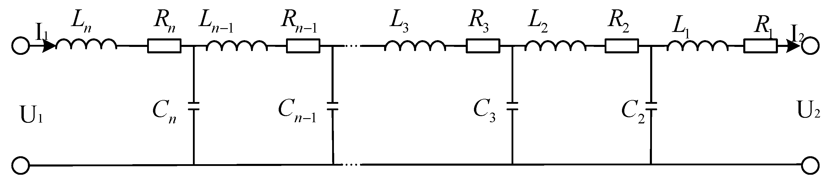
2.2. Circuit Model of Skin Effect Electric Heat Tracing System

To reduce the sensitivity of the skin effect electric heat tracing system in the flow of the oil pipeline, the heat conduction of the oil pipeline is fully realized. According to the tube diameter and the temperature of the heating temperature, the skin effect electric heat tracing system is divided into single tube heating, 120° and 180° double tube heating and three tube heating. To design the circuit parameters of the skin effect electric heating system, such as operating frequency, output voltage, current and power, it is necessary to determine the load impedance circuit of the whole skin effect electric heat tracing system, and the impedance circuit is composed of the heat tracing tube and the heating cable. Because the distance between the heating cable and the heat tracing tube is relatively close, the charge will change on the respective surfaces, there will be stray capacitance, and the length of the whole skin electric heating system can be up to km. According to the circuit principle, when the circuit line length is close to the working wavelength, it is impossible to calculate the characteristics of the circuit by using the centralized parameter circuit model, and it is easy to use the distributed parameter circuit [25]. To facilitate the analysis, assuming that the length of the heat tracing tube is 1000 m and dividing the load into n equal parts, the equivalent circuit is shown in Figure 2.

In Figure 2, the left end is connected to the boosted output of the transformer. I₁ and U₁ are the current and phase voltage at the inlet of the heavy oil. The position at the right end corresponds to the end of the line, and I₂ is the current at the end of the heating cable at the outlet of the heavy oil. With the length of the pipeline, the current amplitude increases steadily, and the maximum value occurs at the end of the pipeline. The currents I₁ and I₂ have the following relationship:

$${\mathrm{I}}_1={\mathrm{I}}_2/\sqrt{2(ch(2\alpha x)+\cos (2\beta x))}$$

(7)

where x is the length of the heat tracing tube and the heating cable, α and β are the real and imaginary parts of the propagation constant γ [26], respectively, i.e.,

$$\gamma =\alpha +\mathrm{j}\beta =\sqrt{(R+\mathrm{j}\omega L)(G+\mathrm{j}\omega C)}$$

(8)

As can be seen from Equation (7), the system current will vary along the pipeline, thereby affecting the generation of heat along the pipeline and the system impedance. In the case of electric heating, the system impedance is mainly the impedance and inductive reactance caused by the skin effect, the eddy current effect, the hysteresis effect of the heat tracing tube, and the impedance and inductive reactance of the heating cable. For the heat tracing tube and the heating cable made of a uniform material, the resistance values, the inductance values, and the respective capacitances are equal, and R, L, and C are respectively set as follows.

$$\begin{array}{c}{R}_1=R_2=\cdots R_n=R\\ L_1=L_2=\cdots L_n=L\\ C_1=C_2=\cdots C_n=C\end{array}$$

(9)

Among the above three variables, C depends only on the material and structure of the conductor, and the size of C will be determined in the case where the material and structure of the heat tracing tube and the heating cable are fixed [27].

$$C=\frac{2\mathsf{\pi }{\epsilon }_0{\epsilon }_{r}l}{\ln (r_2/r_1)}$$

(10)

where r₁ is the radius of the copper core of the cable, r₂ is the inner radius of the heat pipe, l is the length of the pipeline, ε₀ is the vacuum dielectric constant, and ε_r is the dielectric constant of the insulating material.

Under the action of alternating current, eddy current effect, skin effect and hysteresis effect in the heat tracing tube and the heating cable make R and L change. Therefore, the impedance is not only related to length, but also related to material composition, current waveform, current frequency and other factors [11]. For long straight tubular conductors, the magnetic field strength is only the circumferential component, the electric field strength and current density are only axial components, and the field quantity only varies with the radius r due to the symmetry, so the Maxwell equations are in the cylindrical coordinate system.

$$\begin{array}{l}\frac{\mathrm{d}{H}_Q}{\mathrm{d}r}+\frac{H_Q}{r}=\sigma E_Z\\ \frac{\mathrm{d}{E}_Z}{\mathrm{d}r}=j\omega \mu H_Q\end{array}$$

(11)

Among them, H_Q is the circumferential component of the magnetic field strength, E_Z is the electric field strength in the axial direction, σ is the electrical conductivity, and μ is the magnetic permeability. Let $K=\sqrt{\mathrm{j}\omega \sigma \mu }$, which is available

$$\frac{{\mathrm{d}}^2{E}_Z}{\mathrm{d}{(Kr)}^2}+\frac{1}{Kr}\frac{\mathrm{d}{E}_Z}{\mathrm{d}(Kr)}-E_Z=0$$

(12)

Equation (12) is a modified Bessel function, and its general solution is

$$E_Z=A{\mathrm{I}}_0(Kr)+B{\mathrm{K}}_0(Kr)$$

(13)

where I₀ (Kr) is a modified zero-order first-order Bessel function, and K₀ (Kr) is a modified zero-order second-order Bessel function. The values of A and B are obtained from the boundary conditions presented by the full current law.

From Complex Poynting’s Theorem [28], the complex power of the heat pipe is known. The equivalent impedance of the heat pipe is Z = R + jX, so the complex power consumed by the heat pipe can also be expressed as P_c = I²Z. Then its AC (alternating current) impedance is

$$\begin{array}{l}Z=\frac{P_c}{I^2}=\frac{Kl}{2\mathsf{\pi }{r}_2\sigma }·\frac{I_0(K{r}_2)K_1(K{r}_3)+K_0(K{r}_2)I_1(K{r}_3)}{I_1(K{r}_3)K_1(K{r}_2)-K_1(K{r}_3)I_1(K{r}_2)}\\ =R_{0pipe}\frac{K(r_3^2-r_2^2)}{2r_2}·\frac{I_0(K{r}_2)K_1(K{r}_3)+K_0(K{r}_2)I_1(K{r}_3)}{I_1(K{r}_3)K_1(K{r}_2)-K_1(K{r}_3)I_1(K{r}_2)}\end{array}$$

(14)

Among them, R_0pipe = l/(πσ(r₃² − r₂²)) is the DC resistance of the heat tracing tube, r₂ and r₃ are the radii and outer radius of the heat tracing tube, and the real part and imaginary part of (14) are the AC resistance and inductance of the heat tracing tube, respectively. For the heating cable of the cylindrical conductor, the AC impedance of the heating cable can be obtained by the above derivation process.

$$Z=R_{0cable}·\frac{K{r}_1}{2}·\frac{I_0(K{r}_1)}{I_1(K{r}_1)}$$

(15)

where R_0cable = l/(πσ_cabler₁²) is the DC resistance of the heating cable, r₁ is the copper core radius of the cable, and the real and imaginary parts of (15) are the AC resistance and the inductive reactance of the heating cable, respectively. When a heating cable with a cross-sectional area of 25 mm² is selected, the inner radius of the heating cable is r₁ = 2.82 mm, and σ_cable = 59 × 10⁶ S/m. In Reference [29], the heat tracing pipe is a 20# seamless low carbon steel pipe with a specification of Ø27 × 3, σ = 6.29 × 10⁶ S/m, and the distributed circuit parameters of the system can be obtained through the above analysis. The specific circuit parameters and calculation results are shown in

Table 1. Specific measurement parameters and calculation results.

f (kHz)	R(mΩ·m−1)	L(μH·m−1)	α × 10−5	β × 10−5
0.2	5.8	4.365	1.17	2.74
0.5	8.9	2.765	2.30	5.43
1	12.5	1.956	3.83	9.12

.

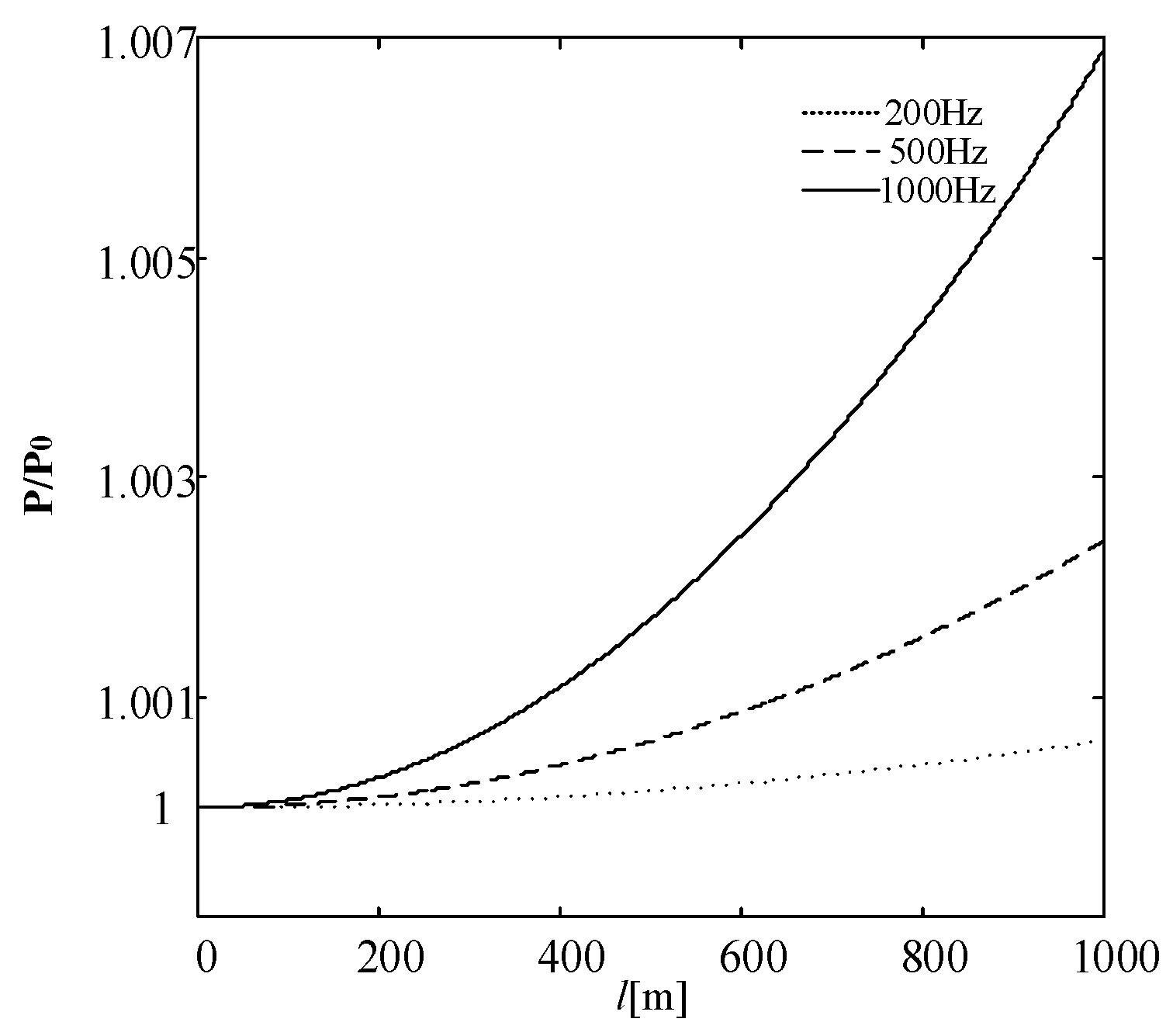
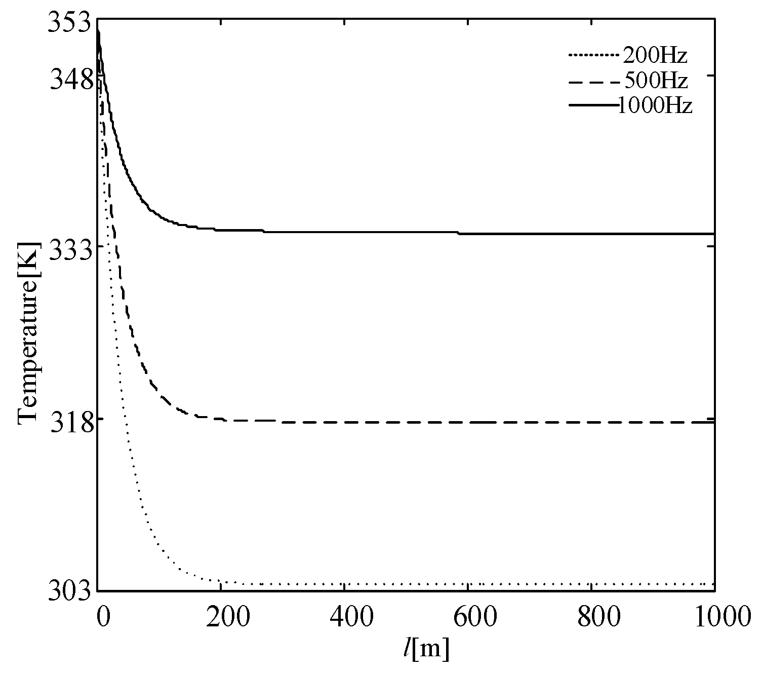
2.3. Effect of Frequency on Electric Heating Efficiency

The heating effect of the skin effect electric tracing system depends on the distributed circuit parameters and current frequency of the system. The circuit parameters calculated in Table 1 are substituted into Equations (7) and (8), and the power calculation formula is utilized. The variation of the power of the heating effect tube and the heating cable with the distance of the pipeline at different current frequencies can be obtained. The simulation curves realized by MATLAB programming are shown in Figure 3.

The variable P is the heating power of each segment of the skin effect electric heat tracing system, and P₀ is the heating power of the heating cable and the heat tracing pipe section at the heavy oil outlet. It can be seen from Figure 3 that when the current frequency is low (200 Hz), the capacitance and inductance are less, and the heat generation of the skin effect electric heating system is improved. In the case of a high current frequency (1000 Hz), the effects of capacitive reactance and inductive reactance are more and more significant, and the power of the skin effect electric heat tracing system exhibits an upward change. At this time, combined with the axial temperature distribution model of the deep-water subsea flowline and the power distribution model of the heating system, the inlet flow rate of the heavy oil is 0.5 m/s, the inlet temperature of the heavy oil is 353 K, and the ambient temperature is 277 K. When being heated by the electric heating, the actual temperature distribution curve of the deep-water submarine pipeline is shown in Figure 4.

It can be seen from the temperature distribution curve of Figure 4 that in the case where the heavy oil inlet temperature, the inlet flow velocity, and the current amplitude is the same, and only the power source frequency is changed, the skin effect electric heat tracing system keeps the temperature of the heavy oil at 303 K or higher. Deep-water flow safety is guaranteed, and it is not difficult to find that the higher the frequency, the slower the oil temperature drop; this indicates that the higher the frequency, the more obvious the skin effect, the greater the equivalent impedance of the distributed circuit parameters of the system, the better the heating efficiency. However, if the frequency is increased without limit, on the one hand, it is limited by the complexity of the power supply device. On the other hand, due to the skin effect, the eddy current heat is limited to the surface layer of the pipe, and then the surface layer is conducted to the heavy oil, and the heating time is elongated. More importantly, when the frequency is increased to a certain value, the electric heating efficiency is in the near-saturation phase, that is, there is a critical frequency. Therefore, the current frequency is not fixed to the maximum, but it should be adjusted according to the change of the load temperature. For this reason, it is necessary to further analyze how to accurately determine the current frequency of the skin effect electric heat tracing system to achieve the optimal heating temperature of the pipeline.

3. Controller Design

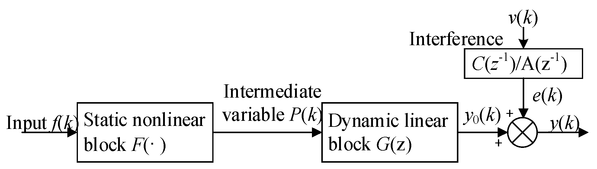
3.1. Predictive Control Based on Hammerstein Model

Because the skin effect electric heat tracing system is a large-lag nonlinear system, and it is difficult to establish its precise mathematical model due to the environment and the composition, flow rate, temperature and other factors of the fluid inside the tube. The traditional controller design method is no longer applicable to the skin effect electric heat tracing system. In Reference [30], the author analyzed the mechanism of the skin effect electric heat tracing system, the magnetic field distribution and equivalent circuit. The heating power is introduced as the intermediate variable to establish the relationship between the power frequency and the fluid temperature. Therefore, the skin effect electric heat tracing system is derived from the Hammerstein model, which consists of a static nonlinear link plus a dynamic linear link [31]. The important derivation process of its Hammerstein model is as follows.

Assuming that the frequency of the current loaded in the heat tracing tube is f, $\overline{B}$ is represented by the average value of the magnetic induction intensity, and the skin effect of the heat tracing tube depends on the characteristics of the material and the power frequency, heating power of the skin effect electric heat tracing system can be obtained [32].

$$P=UI\cos \phi =\frac{1}{4}{\mathsf{\pi }}^3{f}^2\sigma {\overline{B}}^2{\mathrm{r}}_2{}^{4}L=k_0{f}^2$$

(16)

Since the heating efficiency of the skin effect electric heat tracing system is as high as 80% to 90%, it can be assumed that 90% of the system’s heating power is the amount of heat generated. The heat balance equation can be obtained by the law of conservation of energy.

$$0.9P=Gc\frac{\Delta T}{\Delta t}+K_w\mathsf{\pi }Dl\Delta T$$

(17)

The system transfer function can be obtained by applying the Laplace transform on both sides of Equation (17) and adding a purely lagging link.

$$\frac{T(s)}{P(s)}=\frac{k_1}{\tau s+1}{e}^{-t_{0}s}$$

(18)

where k₁ = 0.9/(K_wπDl), τ = Gc/(K_wπDl).

In summary, the nonlinear relationship between the power P and the power frequency is obtained from the perspective of the electromagnetic field, as shown in Equation (16), and is represented by F(·), which can be used as the nonlinear link in the Hammerstein model. The linear relationship between the power P and the fluid temperature is obtained from the perspective of energy conservation, as shown in Equation (18), which can be used as the linear link in the Hammerstein model. Therefore, the structure diagram of the Hammerstein model is shown in Figure 5.

As can be seen from Figure 5, the output of the skin effect electric heat tracing system can be expressed as

$$y(k)=y_0(k)+e(k)$$

(19)

$$y_0(k)=G(z)P(k)$$

(20)

$$P(k)=\{\begin{array}{c}{k}_{0}f{(k)}^2,f(k)\in (0,f_{\max })\\ 0\hspace{1em}\hspace{1em}\hspace{1em},f(k)\in (-\infty ,0)\end{array}$$

(21)

$$e(k)=\frac{C(z^{-1})}{A(z^{-1})}v(k)$$

(22)

where y(k) and e(k) are the output and noise perturbations of the system, y₀(k) and P(k) are unmeasured intermediate variables, and k₀ is the undetermined constant. f(k) is the current frequency of the system. G(z) = z^-dB(z⁻¹)/A(z⁻¹), d is the system delay, v(k) is independent random white noise sequence, and A(z⁻¹), B(z⁻¹), C(z⁻¹) are unit back shift operators z⁻¹ Polynomial. It comes down to the classical Controlled Auto-Regressive Integrated Moving Average (CARIMA).

The skin effect electric heat tracing system is an engineering application system in the field of industrial process control. Because the structure of industrial objects, parameters and environment have great uncertainty, we should not only simply pursue the ideal optimality, but also consider that the control system can still maintain good robustness under the external disturbances. At the same time, it is also necessary to consider the input cost of implementing the control strategy, that is, under the dual requirements of robustness and economy in actual production, predictive control comes into being. The generalized predictive control method can be repeatedly optimized on the basis of actual feedback information; it can take into account the impact of uncertainty, and can be constantly corrected, which is more suitable for the actual process. It can be seen that the generalized predictive control method can be applied to the skin effect electric heat tracing system. The predictive control problem based on Hammerstein model is decomposed into the dynamic optimization problem of the linear model and the static root finding problem of the nonlinear model. The skin effect electric heat tracing system based on the Hammerstein model is obtained by using the generalized predictive control of the linear model to obtain the intermediate variable, and then the control effect in the actual project is inversely calculated by the nonlinear link. Unfortunately, the generalized predictive control needs to set its input and output to be linear and unconstrained, and use gradient optimization to obtain the input of the control increment. However, in the actual industrial process, both the control quantity and the output quantity are bound to be subjected to certain physical constraints. The control quantity and output quantity constraints must be introduced into the optimization algorithm based on the actual situations [33]. It can be seen that it is important to formulate this optimization problem as constrained optimization problem when designing the controller. Based on the Hammerstein model considering the characteristics of the actual physical constraints and the two-step method, the constraints of the input are mapped to the constraints of the intermediate variables, so that the intermediate variables are obtained by the linear predictive control with constraints. Hence, the next step is to study the generalized predictive control method based on the input constraint of the linear part of the Hammerstein model.

3.2. Constrained Generalized Predictive Control

The dynamic linear link (20) and (21) of the Hammerstein model using the skin effect electric heat tracing system are used as prediction models, that is, the CARIMA model can be expressed as.

$$y(k+1)={\displaystyle \sum _{i=1}^n{a}_{1,i}y(k+1-i)+{\displaystyle \sum _{i=0}^m{b}_{1,i}\Delta P(k-d-i)}}+{\displaystyle \sum _{i=0}^r{c}_{1,i}}e(k+1)$$

(23)

The recursion of Equation (23) can determine the minimum variance output prediction value.

$$y=y_m+\mathit{G}\Delta P$$

(24)

where G is the system unit step response coefficient matrix, which is solved by the model coefficients. Therefore, constructing the matrix as follows

$$\mathit{G}=\left[\begin{array}{cccc}{b}_{1,0}& 0& \cdots & 0\\ b_{2,0}& b_{1,0}& \cdots & 0\\ ⋮& ⋮& \cdots & ⋮\\ b_{N-d,0}& b_{N-d-1,0}& \cdots & b_{1,0}\end{array}\right]$$

(25)

$$b_{j,0}=b_{1,j-1}+{\displaystyle \sum _{i=1}^{j_1}{a}_{1,i}{b}_{j-i,0}}\begin{array}{cc}& j=2,3,\cdots ,N-d\end{array}$$

(26)

where j₁ = min{j − 1, n}, and when j − 1 > m, b_1,j−1 = 0, N is the predicted length, and n and m are the highest numbers of A(z⁻¹) and B(z⁻¹) polynomials, respectively. The j-th output prediction sequence y_m(k + j) is completely determined by the past intermediate variables and outputs, and can be derived from

$$y_m\left(k+j\right)={\displaystyle \sum _{i=1}^n{a}_{1,i}{y}_m(k+j-i)+{\displaystyle \sum _{i=0}^m{b}_{1,i}\Delta P(k+j-1-d-i|k)}}+{\displaystyle \sum _{i=0}^r{c}_{1,i}}e(k+j-i|k),j=1,2,\cdots ,N$$

(27)

where,

$$y_m={\left[\begin{array}{cccc}{y}_m(k+d+1)& y_m(k+d+2)& \cdots & y_m(k+N)\end{array}\right]}^T$$

(28)

$$\Delta P={\left[\begin{array}{cccc}\Delta P(k)& \Delta P(k+1)& \cdots & \Delta P(k+N-d-1)\end{array}\right]}^T$$

(29)

$$\Delta P(k+i)=P(k+i)-P(k-1),i=0,1,\cdots ,N-d-1$$

(30)

The reference input trajectory can be calculated in following manner. Let

$$y_r(k+d)=y_m(k+d)$$

(31)

$$y_r(k+d+i)=\alpha y_r(k+d+i-1)+(1-\alpha )W,i=1,2,\cdots ,N-d$$

(32)

$$y_r={\left[\begin{array}{cccc}{y}_r(k+d+1)& y_r(k+d+2)& \cdots & y_r(k+N)\end{array}\right]}^T$$

(33)

where W is the set point and 0 ≤ α ˂ 1, and y_r is the reference trajectory column vector.

Considering input limitation, the input gentle factor β (β ≥ 0) is introduced, and the following relationship exists in one prediction period.

$$\Delta P(k+j)=\left(1+{\displaystyle \sum _{i=1}^j{\beta }^i}\right)\Delta P(k),j=1,2,\cdots N-d-1$$

(34)

Available from Equations (24), (29), and (34)

$$y=y_m+\mathit{G}\mathit{H}\Delta P(k)=y_m+\mathit{g}\Delta P(k)$$

(35)

where, g = GH, $\mathit{H}={\left[\begin{array}{cccc}1& 1+\beta & \cdots & {\displaystyle \sum _{i=0}^{N-d-1}{\beta }^i}\end{array}\right]}^T$

Minimizing the performance index yields the control increment of the current moment without considering the input constraint.

$$\Delta P(k)={\mathit{g}}^T(y_r-y_m)/{\mathit{g}}^T\mathit{g}$$

(36)

Since g^Tg is a scalar, matrix inversion is avoided, which greatly reduces the amount of calculation.

Suppose intermediate variable and its incremental have the following constraints:

$$\begin{array}{l}{P}_{\min }\le P(k+j)\le P_{\max },\\ \Delta P_{\min }\le \Delta P(k+j)\le \Delta P_{\max },j=0,1,\cdots N-d-1\end{array}$$

(37)

The intermediate variables and its incremental constraints can be reduced to a formula based on Equations (34) and (37).

$${\Delta }_{\min }\le \Delta P(k)\le {\Delta }_{\max }$$

(38)

where

$$\begin{array}{l}{\Delta }_{\min }=\max \left\{\begin{array}{cc}\left[P_{\min }-P(k-1)\right]/{\displaystyle \sum _{i=0}^{N-d-1}{\beta }^i},& \Delta P_{\min }/{\displaystyle \sum _{i=0}^{N-d-1}{\beta }^i}\end{array}\right\}\\ {\Delta }_{\max }=\min \left\{\begin{array}{cc}\left[P_{\max }-P(k-1)\right]/{\displaystyle \sum _{i=0}^{N-d-1}{\beta }^i},& \Delta P_{\max }/{\displaystyle \sum _{i=0}^{N-d-1}{\beta }^i}\end{array}\right\}\end{array}$$

(39)

It can be seen that after the input softening factor is introduced, no matter how the prediction length changes, the number of constraints is only one, and the variable is ΔP(k). Therefore, it is not necessary to use nonlinear search to solve the nonlinear programming problem.

Therefore, when implementing the input-constrained generalized predictive control algorithm, the intermediate increment ΔP(k) under the unconstrained condition is first calculated according to Equation (36), and then it is judged whether the control increment satisfies the constraint condition. When ΔP(k)∊[Δ_min, Δ_max], the increment of the constrained intermediate variable is consistent with the solution under unconstrained conditions; when ΔP(k)∉[Δ_min, Δ_max] the increment of the constrained intermediate variable is taken as the nearest critical value, i.e.,

$$\Delta P(k)=\{\begin{array}{ll}{\Delta }_{mim},\hfill & \Delta P(k)<{\Delta }_{mim}\hfill \\ {\Delta }_{\max },\hfill & \Delta P(k)>{\Delta }_{\max }\hfill \\ \Delta P(k),\hfill & \mathrm{other}\hfill \end{array}$$

(40)

Thereby, the control law at time k can be determined

$$P(k)=P(k-1)+\Delta P(k)$$

(41)

The control algorithm proposed above can be summarized as follows.

• Step 1. The unknown parameter in Equation (23) is required for parameter identification. If the model parameters are known, this step is omitted.
• Step 2. Under the unconstrained condition, the optimal control increment ΔP(k) at the current moment is obtained by Equation (36).
• Step 3. Determine whether the set value satisfies the constraint condition (38), if ΔP(k) ∊ [Δ_min, Δ_max], go to Step 5.
• Step 4. If ΔP(k) ∉ [Δ_min, Δ_max], the corresponding processing is performed according to Equation (40).
• Step 5. Calculate and implement the current control variable P(k) by Equation (41).
• Step 6. At the next sampling moment, return to Step 1.

Through the above analysis, the intermediate variable P(k) can be obtained, and then the control quantity f(k) is solved inversely according to the nonlinear link of the Hammerstein model. For the characteristics of Hammerstein model, and the power frequency and the heating power of the pipeline are both positive, and there must be a unique inverse function F⁻¹(·) of F(·). Therefore, the control quantity f(k) can be directly solved by solving the equation, and the control quantity is within the constraint range, so that the control action can be implemented.

3.3. System Stability Analysis

Considering the dynamic linear link of the Hammerstein model, since the white noise disturbance does not affect the closed-loop stability of the system, the noise term is set to zero, and the linear link discrete process is described.

$$(1+a_1{z}^{-1}+\cdots +a_n{z}^{-n})y(k)=z^{-d}(b_1+b_2{z}^{-1}+\cdots +b_m{z}^{-(m-1)})\Delta P(k-1)$$

(42)

The state space expression of Equation (41) is described as Equation (43).

$$\{\begin{array}{ccc}\hfill x(k+1)& =& \mathit{A}x(k)+\mathit{B}\Delta P(k-d)\hfill \\ \hfill y(k)& =& \mathit{C}x(k)\hfill \end{array}$$

(43)

Among them

$$\mathit{A}=\left[\begin{array}{cccc}-a_1& \cdots & -a_{n-1}& -a_n\\ 1& \cdots & 0& 0\\ ⋮& \ddots & ⋮& ⋮\\ 0& \cdots & 1& 0\end{array}\right],\mathit{B}=\left[\begin{array}{c}1\\ 0\\ ⋮\\ 0\end{array}\right],{\mathit{C}}^T=\left[\begin{array}{c}{b}_1\\ b_2\\ ⋮\\ b_n\end{array}\right]$$

(44)

The state and output value of the d step after the current time k are described by Equation (45).

$$\{\begin{array}{l}x(k+d+j)={\mathit{A}}^{d}x(k+j)+[{\mathit{A}}^{j-1}\mathit{B},\cdots ,\mathit{B}]{[\Delta P(k),\cdots ,\Delta P(k+j-1)]}^T\\ y(k+d+j)=\mathit{C}x(k+d+j)\end{array}$$

(45)

When j varies between 1 and N, its vector form can be described as follows.

$$Y=Y_m+\mathit{G}\Delta P$$

(46)

Among them

$$\begin{array}{l}Y={[y(k+d+1),y(k+d+2),\cdots ,y(k+d+N)]}^T\hfill \\ Y_m={\mathit{K}}_{\mathit{m}}x(k+d)\hfill \\ \Delta P=[\Delta P(k),\Delta P(k+1),\cdots ,\Delta P(k+N-1)]\hfill \\ {\mathit{K}}_m=\left[\begin{array}{c}\mathit{CA}\\ {\mathit{CA}}^2\\ ⋮\\ {\mathit{CA}}^N\end{array}\right],\mathit{G}=\left[\begin{array}{cccc}\mathit{CB}& 0& 0& 0\\ \mathit{CAB}& \mathit{CB}& 0& 0\\ ⋮& \ddots & \ddots & 0\\ {\mathit{CA}}^{N-1}\mathit{B}& \cdots & \mathit{CAB}& \mathit{CB}\end{array}\right]\hfill \end{array}$$

(47)

where, Y_m is the predicted output of the system at a future time, and N is the predicted length. At the same time, the input softening coefficient β is defined to constrain the intermediate variables.

$$\Delta P(k+j)=(1+{\displaystyle \sum _{i=1}^j{\beta }^i})\Delta P(k),j=1,2,\cdots ,N-d-1$$

(48)

The expression of the output is obtained by Equations (46), (47) and (48).

$$Y=Y_m+\mathit{GH}\Delta P=Y_m+\mathit{g}\Delta P$$

(49)

where

$$\begin{array}{ccc}\hfill \mathit{H}& =& {\left[1,1+\beta ,\cdots ,1+\beta +\cdots +{\beta }^{N-d-1}\right]}^T,\beta \ge 0\hfill \\ \hfill \mathit{g}& =& \mathit{GH}={\left[g_1,g_2,\cdots ,g_{N-d}\right]}^T\hfill \end{array}$$

(50)

The conventional predictive control performance index is J =‖e(k)‖²+r‖∆P(k)‖², and the input softening coefficient β is more intuitive than the input weighting matrix r of the conventional predictive control performance index. Therefore, the objective function is shown as follows.

$$J={(Y-Y_r)}^T(Y-Y_r)$$

(51)

where, Y_r is the reference trajectory, which is defined as follows.

$$\begin{array}{l}{Y}_r={[y_r(k+d+1),y_r(k+d+2),\cdots ,y_r(k+d+N)]}^T\hfill \\ y_r(k+d)=y(k+d)\hfill \\ \begin{array}{c}{y}_r(k+d+j)=\alpha y_r(k+d+j-1)+(1-\alpha )s,\\ j=1,2,\cdots ,N\end{array}\hfill \end{array}$$

(52)

where, α (0 < α < 1) is the output softening coefficient and s is the set value of the desired output of the system.

$$\begin{array}{l}{Y}_r={\mathit{K}}_{\mathit{r}}x(k+d)+{\mathit{T}}_{\mathit{r}}s\hfill \\ {\mathit{K}}_{\mathit{r}}={[\alpha ,{\alpha }^2,\cdots ,{\alpha }^N]}^{T}C\hfill \\ {\mathit{T}}_{\mathit{r}}=[1-\alpha ,1-{\alpha }^2,\cdots ,1-{\alpha }^N]\hfill \end{array}$$

(53)

Let $\partial J(\Delta P(k))/\partial (\Delta P(k))=0$, and the ΔP(k) can be obtained, the objective function is minimized.

$$\Delta P(k)={({\mathit{g}}^T\mathit{g})}^{-1}{\mathit{g}}^T(Y_r-Y_m)$$

(54)

Substituting Equation (47) and Equation (53) into Equation (54), the increment of the intermediate variable is obtained.

$$\Delta P(k)={({\mathit{g}}^T\mathit{g})}^{-1}{\mathit{g}}^T[({\mathit{K}}_{\mathit{r}}-{\mathit{K}}_{\mathit{m}})x(k+d)+{\mathit{T}}_{\mathit{r}}s]=\mathit{K}x(k+d)+\mathit{T}s$$

(55)

where, K = (g^Tg)⁻¹g^T(K_r − K_m), T = (g^Tg)⁻¹g^TT_r, and K_r, K_m are both N × n dimensional matrix. K is n-dimension row vector, let K = [k₁, k₂, …k_n], and T is scalar.

By substituting Equation (55) into the state space model described by Equation (43), the closed-loop equation of the generalized predictive control system can be obtained.

$$\{\begin{array}{ccc}\hfill x(k+1)& =& (\mathit{A}+\mathit{BK})x(k)+\mathit{BT}s\hfill \\ \hfill y(k)& =& \mathit{C}x(k)\hfill \end{array}$$

(56)

The closed-loop transfer function from the set value to the output is obtained from Equation (56).

$$G_c(z)=\mathit{C}{(z\mathit{I}-\mathit{A}-\mathit{BK})}^{-1}\mathit{BT}=\frac{(b_1+b_2{z}^{-1}+\cdots +b_m{z}^{-(m-1)})\mathit{T}}{1+(a_1-k_1)z^{-1}+\cdots +(a_n-k_n)z^{-n}}$$

(57)

The closed-loop characteristic equation of the system is obtained.

$$1+(a_1-k_1)z^{-1}+\cdots +)a_n-k_n)z^{-n}=0$$

(58)

Therefore, the necessary and sufficient condition for the closed-loop stability of the generalized predictive control system is that the closed-loop characteristic roots are uniformly distributed in the unit circle of the z-plane, and the system makes the characteristic roots within the unit circle of the z-plane by reasonably selecting the softening coefficients α and β. It can be seen from Equation (55) that generalized predictive control is a state feedback control, and the closed-loop system is stabilized by state feedback.

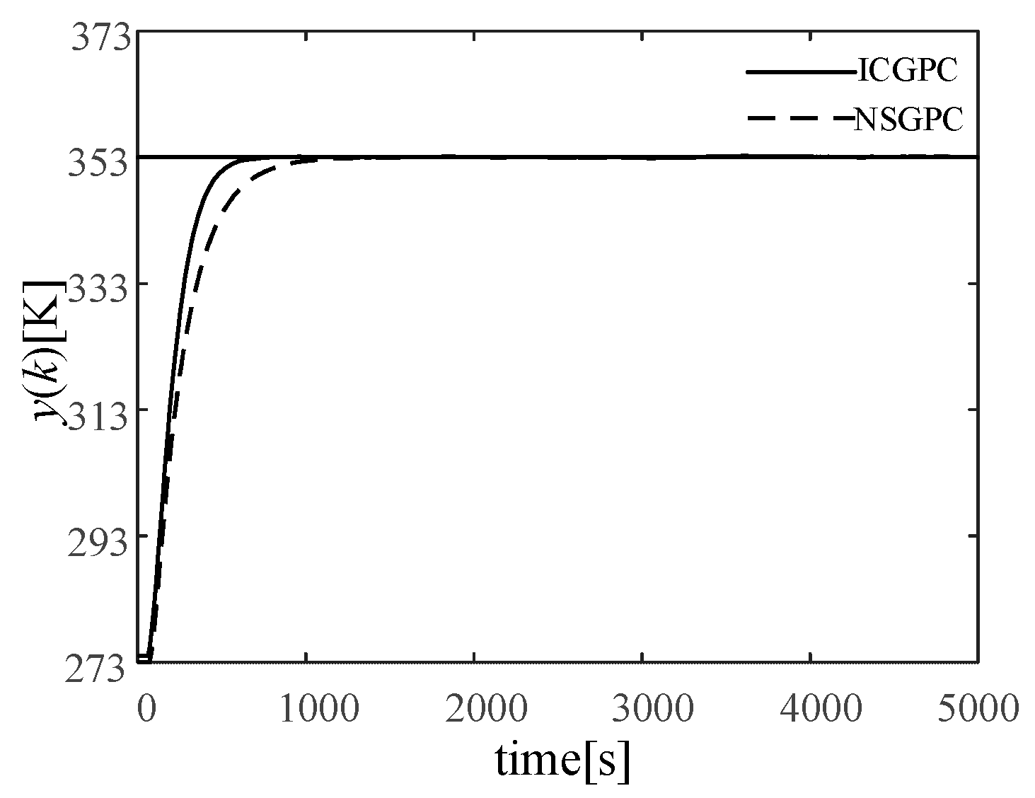
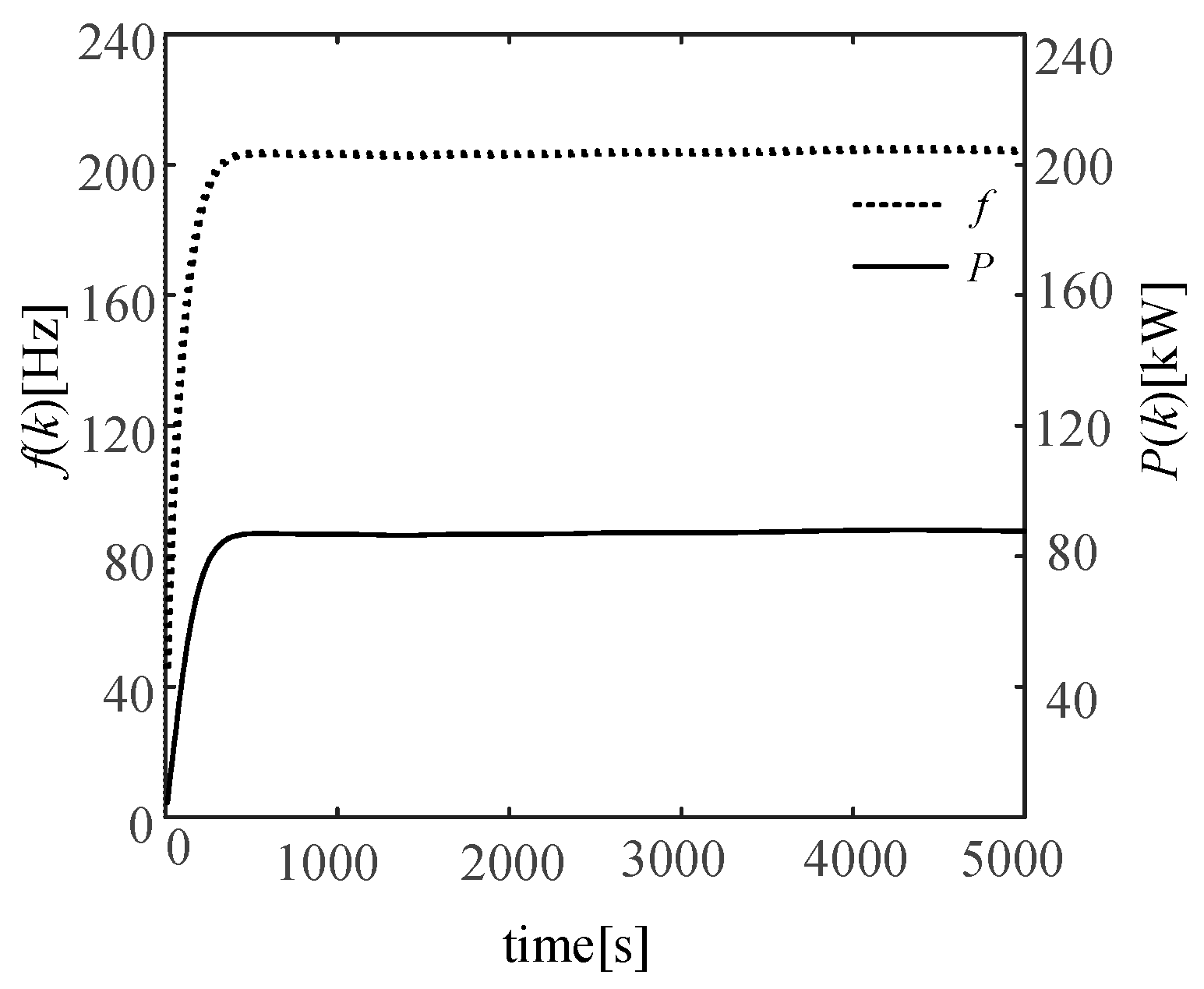
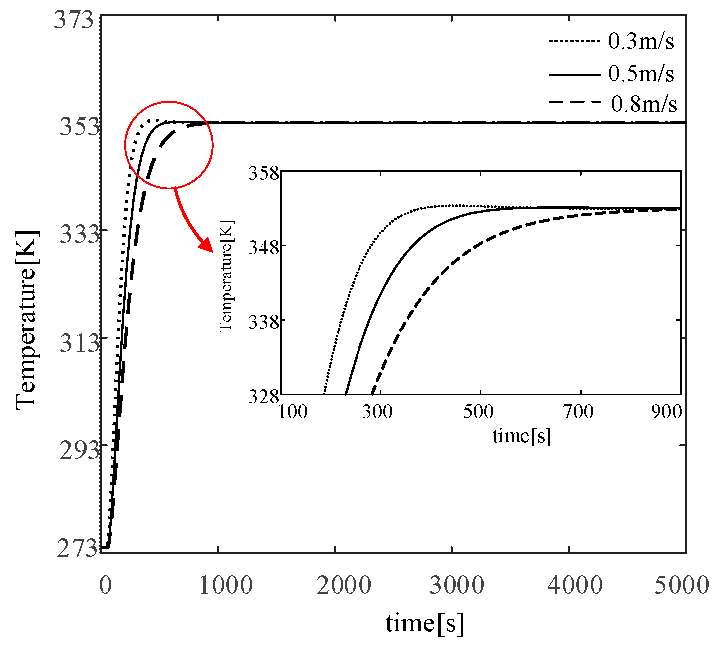
4. Simulation Verification

This study used the parameters values in a pipeline project [34]: the pipe size is Ø219 × 7 mm, the length is 1000 m, the thickness of the insulation layer is 20 mm, and its thermal conductivity is 0.04 W/(m·K), the inlet flow rate of the oil is 0.5m/s, the inlet temperature of the oil is 353 K, and the ambient temperature is 277 K. The total heat transfer coefficient between crude oil and seawater is calculated as K_w = 1.81 W/(m²·K), and the mass flow rate of crude oil is G = 14.1 kg/s. The collected sample data was selected and optimized by the Hammerstein model using the standard particle swarm optimization algorithm to determine the Hammerstein model of the skin effect electric heat tracing system. The identification parameters are set to window width L_w = 100, particle number N = 20, inertia weight w (t) = 0.9 − 0.5t/MaxNumber, learning factor parameter initial value c₁ = c₂ = 0.15, search precision to 0.01, and maximum evolution algebra to be 1000 generations; parameters after multiple simulations are shown in

Table 2. Various identification results against interference of noise.

Parameters	Actual Value	Estimates for Different Disturbances
		0.1	0.2	0.3	0.4
k0	2.1	2.1003	2.0984	2.1007	2.1004
a1	−0.670	−0.669	−0.672	−0.669	−0.668
b1	0.0003	0.0002	0.0003	0.0004	0.0002
d	6	6.0021	6.0021	5.9947	6.0000

.

Therefore, the Hammerstein model of the skin effect electric heat tracing system is determined.

$$F(f(k))=\{\begin{array}{c}2.1f{(k)}^2,f(k)\in (0,f_{\max })\\ 0\hspace{1em}\hspace{1em}\hspace{1em},f(k)\in (-\infty ,0)\end{array}$$

(59)

$$G(z)=\frac{0.0003}{z-0.6703}{z}^{-6}$$

(60)

The skin effect electric heating system test shows that when the current frequency is 500 Hz, the penetration depth is 0.3 mm, and the wall thickness of the conventional heat tracing tube is 3 mm, and the skin effect phenomenon is very significant. At this time, increasing the frequency does not greatly improve the heat generation of the heat tracing tube, and has reached its critical value. Therefore, the current frequency takes the range of 50 Hz ≤ f(k) ≤ 500 Hz, and the current frequency change rate fluctuates at ±0.5 Hz, thereby determining the constraint of the heating power P(k), that is, 5.25 kW ≤ P(k) ≤ 525 kW, −1.05 ≤ ΔP(k) ≤ 1.05.

To compare the control effects, the nonlinear separation method generalized predictive control (NSGPC) for selecting nonlinear quadratic programming optimization is compared with the generalized predictive control designed by introducing the input softening factor method (ICGPC). The difference between the two is that ICGPC calculates the intermediate increment ΔP(k) under unconstrained condition by Equation (36), and then judges whether the control increment satisfies the constraint condition, and after obtaining the intermediate variable constraint, NSGPC solves the intermediate variable by establishing the following performance index.

$$\begin{array}{c}\underset{\Delta P(k|k),\cdots \Delta P(k+N_u-1|k)}{\min }J(k)={\displaystyle \sum _{i=N_1}^{N_2}{[y(k+i|k)-y_s(k+i)]}^2}+{\displaystyle \sum _{j=1}^{N_u}\lambda \Delta P^2(k+j-1|k)}\\ s.t.\Delta P(k+l|k)=0,l\ge N_u\\ P_{\min }\le \Delta P(k+j-1|k)\le P_{\max },j\in \left\{1,\cdots ,N_u\right\}\end{array}$$

(61)

where y_s(k + j) is the reference value for future output, N₁ and N₂ are the start and end times of the prediction time domain, N_u is the control time domain, and λ is the control weighting coefficient, which makes it easy to see the difference between ICGPC and NSGPC. The dynamic linear link of the Hammerstein model is controlled by using the ICGPC method, where the controller parameter is taken as: N = 12, d = 6, α = 0.7, β = 2.1. The simulation duration is 500 sampling moments, the sampling time is 10s. To further investigate the anti-interference ability of the control strategy, the interference signal is white noise driven linear filter C(z⁻¹)/A(z⁻¹) = (1 + 0.5z⁻¹)/(1 − 0.6703z⁻¹), which is added to obtain the curve of output over time as shown in Figure 6.

It can be seen from Figure 6 that the constrained generalized predictive control (GPC) controller designed by introducing the input softening factor method can make the system reach the set temperature of 353 K in about 500 s, the dynamic response is fast, and the system static error is reduced to almost zero after 600 s. The nonlinear generalized predictive control NSGPC using quadratic programming optimization needs to calculate the inversion of the Diophantine equation and the matrix, leading to high computation cost. Therefore, the steady state is reached in about 1000 s. It can be seen that the comparison of ICGPC and NSGPC shows that the method that relies on the input softening factor is more advantageous.

Under the action of the ICGPC, the simulation results are shown in Figure 7. The system power frequency f is represented by the dashed line, and the system intermediate variable heating power P is represented by the solid line. At the same time, it can be seen from the simulation that the system frequency is 200 Hz when the system’s heating temperature is maintained at 353 K, and the heating power required by the system is maintained at about 85 kW. Therefore, it is possible to design an intermediate frequency heating power source with a maximum heating power of 100 kW which provides a certain theoretical guidance for the design of the heating power supply for the skin effect electric heating system, thereby avoiding the drawbacks of the above parameters can only be estimated according to engineering experiments.

To fully demonstrate that the ICGPC gets rid of the previous control based on strict mathematical model requirements, the object parameters are changed to examine adaptive adjustment capabilities of the system. Since the inlet velocity of heavy oil is closely related to the system model parameters. According to the analysis, when the flow rate increases, the model parameter a₁ increases, and b₁ decreases, which will cause the linear part of the Hammerstein model to change, thus changing the object model as a whole. Therefore, three inlet flow rates were selected, which were 0.3 m/s, 0.5 m/s and 0.8 m/s, respectively. The only changed parameter is the flow rate during the simulation, and other control parameters remain unchanged. The temperature curves of different flow rates are shown in Figure 8.

As can be seen from Figure 8, as the flow rate increases, it takes longer for the system to reach the target heating temperature. This is due to the lack of the heat conduction time of the heavy oil in the pipe, so that the temperature rises slowly. When the values of N, d, α and β in the ICGPC are kept the same, and the outlet temperature can still maintain at 353K. Therefore, the system can still maintain the steady state under the changes of the model parameters, indicating that the system has strong adaptive ability. According to the analysis, ICGPC can tolerate the unknown dynamic changes of the system to a large extent.

5. Conclusions

The analysis of the axial temperature distribution model of submarine pipelines shows that the sensitivity of the skin effect electric heat tracing system to the oil delivery is reduced, and the delivery temperature of the external pipeline can be controlled, so that the deep-water flow safety can be guaranteed. The distribution parameter model of the skin effect electric heat tracing system is established, and the impedance values of the heat pipe and the heating cable at different frequencies are calculated, and the influence of the frequency on the heating efficiency of the heat pipe is analyzed. The actual temperature distribution of the submarine pipeline is obtained by combining the submarine pipeline temperature field and the skin effect electric heat tracing system power distribution, indicating that the heating effect of the skin effect electric tracing system depends on the distributed circuit parameters and current frequency of the system. Temperature control of skin effect electric tracing system is based on Hammerstein model. The model relies on the change of load temperature to adjust the current frequency change, the generalized predictive control of the input softening factor can be applied to obtain the theoretical values of heating power and current frequency, which avoids the disadvantage that the above parameters are only estimated according to engineering experiments. Moreover, the generalized predictive control of the input softening factor can make the system reach the target temperature, the dynamic response is fast, and the system static error is reduced to almost zero. Therefore, the pipeline heating is efficient and stable, and can quickly respond to the disturbance of the system by overcoming the change of working conditions, thereby realizing the scientific operation and management.

References

1. Wang, D. Comparison and analysis of active heating technology in deep-water subsea flow line. Petro- Chem. Equip. 2016, 45, 64–68. Available online: http://www.cnki.com.cn/Article/CJFDTotal-SYSB201603015.htm (accessed on 26 June 2019).
2. Havre, K.; Stornes, K.O.; Stray, H. Taming slug flow in pipelines. ABB Rev. 2000, 4, 55–63. [Google Scholar]
3. Malekzadeh, R.; Henkes, R.; Mudde, R.F. Severe slugging in a long pipeline–riser system: Experiments and predictions. Int. J. Multiph. Flow 2012, 46, 9–21. [Google Scholar] [CrossRef]
4. Zhou, X.; Shi, Y. Study of Subsea Pipeline Heat Tracing Technology. Pipeline Tech. Equip. 2017, 5, 53–56. [Google Scholar]
5. Guo, X.; Wu, Z.; Shi, Z. Research and application of skin-effect current tracing in submarine pipeline. In Proceedings of the Fifteenth China Ocean (Ashore) Engineering Symposium (Part II), Taiyuan, China, 3–6 August 2011; pp. 1488–1490. [Google Scholar]
6. Li, P.; Zhou, X.; Zhou, X.; Wang, D.; Li, H. Design discussion on the flow assurance for transportation pipelines of high pour point crude oil. Oil-Gas Field Surface Eng. 2018, 37, 52–55. Available online: http://www.cnki.com.cn/Article/CJFDTotal-YQTD201802018.htm (accessed on 26 June 2019).
7. Trichtchenko, L. Modeling electromagnetic induction in pipelines. In Proceedings of the CORROSION 2004, New Orleans, LA, USA, 28 March–1 April 2004; pp. 1–13. [Google Scholar]
8. Lervik, J.K.; Børnes, A.H.; Nysveen, A.; Høyer-Hansen, M. Electromagnetic modelling of steel pipelines for DEH applications. In Proceedings of the Seventeenth International Offshore and Polar Engineering Conference, Lisbon, Portugal, 1–6 July 2007; pp. 1014–1018. [Google Scholar]
9. Ahlen, C.H.; Torkildsen, B.; Klevjer, G.; Lauvdal, T.; Lervik, J.K.; Ronningen, K. Electrical Induction Heating System of Subsea Pipelines. In Proceedings of the Second International Offshore and Polar Engineering Conference, San Francisco, CA, USA, 14–19 June 1992; pp. 78–85. [Google Scholar]
10. Sun, M.; Fang, X.; Zheng, N.; Kang, Q. Research on electric heating special frequency converter for heavy oil exploitation. J. Univ. Pet. 2003, 27, 116–118. [Google Scholar]
11. Fang, X.; Sun, M.; Xu, W.; Yang, G.; Chang, F.; Cheng, J. Theoretical analysis and practice of an energy-saving method in heavy oil thermal recovery. J. Tsinghua Univ. 2003, 43, 891–894. Available online: http://www.cnki.com.cn/Article/CJFDTotal-QHXB200307008.htm (accessed on 26 June 2019).
12. Lervik, J.K.; Iversen, Ø.; Solheim, K.T. Optimizing electrical heating system of subsea oil production pipelines. In Proceedings of the 28th International Ocean and Polar Engineering Conference, Sapporo, Japan, 10–15 June 2018; pp. 108–113. [Google Scholar]
13. Yin, Z.; Wang, X.; Wu, J. Study of large skin effect power tracing system. J. Zhejiang Univ. 2004, 38, 636–639. [Google Scholar]
14. Ding, L.; Zhang, J.; Lin, A. Modeling and control strategy of skin effect electric tracing system. Acta Petrolei Sinica 2018, 39, 837–844. [Google Scholar] [CrossRef]
15. Xu, X. Adaption Control and Model Predictive Control; Tsinghua University Press: Beijing, China, 2017; pp. 216–218. ISBN 978-7-302-44922-5. [Google Scholar]
16. Demircloglu, H. Constrained continuous-time generalised predictive control. IEE Proc.: Control Theory Appl. 1999, 146, 470–476. [Google Scholar] [CrossRef]
17. Zhang, Q.; Li, S. Constrained generalized predictive control using genetic algorithm. J. Shanghai Jiaotong Univ. 2004, 38, 1562–1566. [Google Scholar]
18. Tong, C.; Xiao, L.; Peng, K.; Li, J. Constrained generalized predictive control of mould level based on genetic algorithm. Control Decis. 2009, 24, 1735–1739. Available online: http://www.cnki.com.cn/Article/CJFDTotal-KZYC200911026.htm (accessed on 26 June 2019).
19. Smoczek, J.; Szpytko, J. Constrained generalized predictive control with particle swarm optimizer for an overhead crane. In Proceedings of the International Conference on Methods & Models in Automation & Robotics (MMAR), Miedzyzdroje, Poland, 28–31 August 2017; pp. 756–761. [Google Scholar]
20. Smoczek, J.; Szpytko, J. Particle Swarm Optimization-Based Multivariable Generalized Predictive Control for an Overhead Crane. IEEE/ASME Trans. Mechatron. 2017, 22, 258–268. [Google Scholar] [CrossRef]
21. Jin, Y. New generalized predictive control with input constraints. Control Decis. 2002, 17, 506–508. Available online: http://www.cnki.com.cn/Article/CJFDTotal-KZYC200204032.htm (accessed on 26 June 2019).
22. Su, B. Constrained Fuzzy Predictive Control for the Nonlinear System. Ph.D. Thesis, Nankai University, Tianjin, China, 2006. [Google Scholar]
23. Archer, R.A.; Osullivan, M. Models for heat transfer from a buried pipe. SPE 1997, 2, 186–193. [Google Scholar] [CrossRef]
24. Yang, X.; Chen, L.; Wang, F.; Liu, J. Characteristics of Salinity Distribution in Surface Seawater of the Oceans. J. Oceanogr. Taiwan Strait 1990, 9, 88–91. [Google Scholar]
25. Sun, M.; Zheng, N.; Fang, X.; Kang, Q.; Li, Z.; Wang, L.; Sun, Y.; Yao, C. Research on high-efficiency methods of electrical heating in gathering heavy oil. Acta Phys. Sin. 2002, 51, 2906–2910. [Google Scholar]
26. Qiu, G. Circuit Principle, 5th ed.; Higher Education Press: Beijing, China, 2006; pp. 480–484. ISBN 978-7-04-019671-9. [Google Scholar]
27. Paul, C.R. Analysis of Multi Conductor Transmission Lines, 2nd ed.; John Wiley & Sons, Inc.: Hoboken, NJ, USA, 2008; pp. 110–158. ISBN 978-0-470-13154-1(cloth). [Google Scholar]
28. Guo, L. Study on Characteristic Mode Theory for Composite Electromagnetic Structures and its Applications. Ph.D. Thesis, University of Electronic Science & Technology of China, Chengdu, China, 2018. [Google Scholar]
29. Tang, X. Research of Skin Effect Current Tracing Controlling System on Oil Pipelines. Master’s Thesis, China Jiliang University, Hangzhou, China, 2014. [Google Scholar]
30. Ding, L.; Zhang, J.; Sun, H. Modeling and control strategy of built-in skin effect electric tracing system. CMES 2018, 117, 213–229. [Google Scholar] [CrossRef]
31. Ding, B. Theory and Method of Predictive Control, 2nd ed.; China Machine Press: Beijing, China, 2017; pp. 61–63. ISBN 978-7-111-56002-9. [Google Scholar]
32. Liao, S. Ferromagnetics, 2nd ed.; Science Press: Beijing, China, 1988; pp. 6–21. ISBN 703-0-002-318. [Google Scholar]
33. Muthukumar, N.; Srinivasan, S.; Ramkumar, K.; Kavitha, P.; Balas, V.E. Supervisory GPC and evolutionary PI controller for web transport systems. Acta Polytech. Hung. 2015, 12, 135–153. [Google Scholar]
34. Chen, Z.; Huang, J.; He, Y.; Wang, Z.; Liu, H. Non-uniform temperature fields of a deep-sea pipeline in steady flow. J. Harbin Eng. Univ. 2017, 38, 189–194. [Google Scholar] [CrossRef]
Figure 1. Temperature distribution curve of heavy oil pipeline.
Energies 12 02466 g001
Figure 2. Equivalent model of distributed parameter circuit.
Energies 12 02466 g002
Figure 3. Power curve at different frequencies.
Energies 12 02466 g003
Figure 4. Temperature distribution curve.
Energies 12 02466 g004
Figure 5. The structure diagram of Hammerstein model.
Energies 12 02466 g005
Figure 6. Output curve of constrained generalized predictive control. ICGPC: input softening factor to design constrained generalized predictive control; NSGPC: the nonlinear separation method generalized predictive control.
Energies 12 02466 g006
Figure 7. Response curve of system control variable f(k) and intermediate variable P(k).
Energies 12 02466 g007
Figure 8. Temperature curves with different flow rates.
Energies 12 02466 g008