Viscosity–Temperature–Pressure Relationship of Extra-Heavy Oil (Bitumen): Empirical Modelling versus Artificial Neural Network (ANN)

Abstract

The viscosity data of two heavy oil samples X and Y, with asphaltene contents 24.8% w/w and 18.5% w/w, respectively, were correlated with temperature and pressure using empirical models and the artificial neural network (ANN) approach. The viscosities of the samples were measured over a range of temperatures between 70 °C and 150 °C; and from atmospheric pressure to 7 MPa. It was found that the viscosity of sample X, at 85 °C and atmospheric pressure (0.1 MPa), was 1894 cP and that it increased to 2787 cP at 7 MPa. At 150 °C, the viscosity increased from 28 cP (at 0.1 MPa) to 33 cP at 7 MPa. For sample Y, the viscosity at 70 °C and 0.1 MPa increased from 2260 cP to 3022 cP at 7 MPa. At 120 °C, the viscosity increased from 65 cP (0.1 MPa) to 71 cP at 7 MPa. Notably, using the three-parameter empirical models (Mehrotra and Svrcek, 1986 and 1987), the correlation constants obtained in this study are very close to those that were previously obtained for the Canadian heavy oil samples. Moreover, compared to other empirical models, statistical analysis shows that the ANN model has a better predictive accuracy (R² ≈ 1) for the viscosity data of the heavy oil samples used in this study.

1. Introduction

Viscosity is a crucial parameter in engineering design and simulation, which is useful in the recovery, production, and transportation operations of heavy and extra-heavy oils including bitumen [1,2,3,4,5,6,7]. In addition, extra-heavy oil (bitumen) exists under pressure in the reservoir [8], and viscosity affects its mobility and production flow [9,10]. Thus, several efforts have been directed toward the prediction of the viscosity of bitumen (and of mixtures with solvents) at various temperatures and pressures [2,3,4,6,7,8,11,12,13,14,15,16].

The three-parameter empirical correlations for the viscosity–temperature–pressure relationship originally developed for Athabasca and Cold Lake extra-heavy oil (bitumen), which was proposed by Mehrotra and Svrcek [6,7], are probably the most popular functions that have been applied for the prediction of the viscosity of compressed bitumen [12,16]. In an extension of the above, Puttagunta et al. [8] proposed a modification of these correlations for the prediction of a new set of viscosity data for various bitumen samples obtained from Canadian heavy oil deposits over a range of temperatures between 20 °C and 120 °C and pressures between 0.1 MPa and 18 MPa. Other reported functions for the prediction of viscosity of extra-heavy oil at different temperatures and pressures include those that were used by Appeldorn [17], Alade et al. [14], Farobie et al. [18], and Barus [19] that have been reviewed elsewhere in the literature [12,16].

In recent times, artificial neural networks (ANNs) have been widely used in various physical sciences and engineering applications as a tool for estimating the nonlinear relationship between the input and output data due to their ability to approximate arbitrary nonlinear functions [20,21,22]. As illustrated in Figure 1, the operating mechanism and/or information processing methodology of ANNs are believed to be inspired by the working process of the human brain; thus, they are capable of learning from complex interrelationships between dependent and independent variables [18,21,22,23,24].

In addition, an ANN represents a quick and efficient method to modeling the mathematical relationships between the independent and dependent variables of a process [25,26,27]. Moreover, using an ANN tool offers a number of advantages over the mechanistic models including the non-requirement of the mathematical description of the phenomena involved. The technique has also been found useful in solving various problems in different aspects of the petroleum industry [28,29,30,31,32,33,34,35,36].

The present effort aims at the viscosity modeling of extra-heavy oil using selected empirical functions and an ANN tool with the main interest in validating the models and establishing their accuracy for predicting viscosity at different temperatures and pressures compared to the ANN prediction tool.

2. Materials and Methods

2.1. Materials

The bitumen samples used in this study were obtained from two different locations within the bitumen belt in Ondo State, Southwest Nigeria, namely, Agbabu (sample X) at latitudes of 6° 39′ and 40’ N and longitudes of 4° 53′ and 25′ E and Loda (sample Y) at latitudes of 5° 45′ and 5° 50′ N and longitudes of 4° 00′ and 4° 20′ East. The Agbabu bitumen sample was a semi-solid extra heavy oil which was scooped from an uncapped borehole. The sample to be used for the experiment was dewatered by heating briefly in an environment-controlled oven (OFW-300B, Ettas, AS-ONE, Tokyo, Japan) to liberate the free water content. Drying was done at 60 °C for 10 min in a container purged with nitrogen gas. In the case of the Loda sample, bitumen was extracted from the outcrop using toluene. The toluene was then removed by evaporation in the OFW-300B oven at 50 °C and continuously weighed until the weight loss was negligible. As detailed in

Table 1. Properties of Nigerian oil sands and bitumen. API.

Properties	X	Y
Bitumen content (% w/w)	83.42	45.75
Water content (% w/w)	15.14	33.48
Mineral matter (% w/w)	1.44	20.76
Asphaltene (% w/w)	24.83	18.50
Molecular mass (kg/mol)	748	-
Specific gravity (S.G. 25 °C/25 °C)	1.02	1.01
API gravity	7.2	8.6

Source: Adebiyi and Omode [37].

, the physico-chemical properties of the samples are available elsewhere in the literature [37].

2.2. Methodology

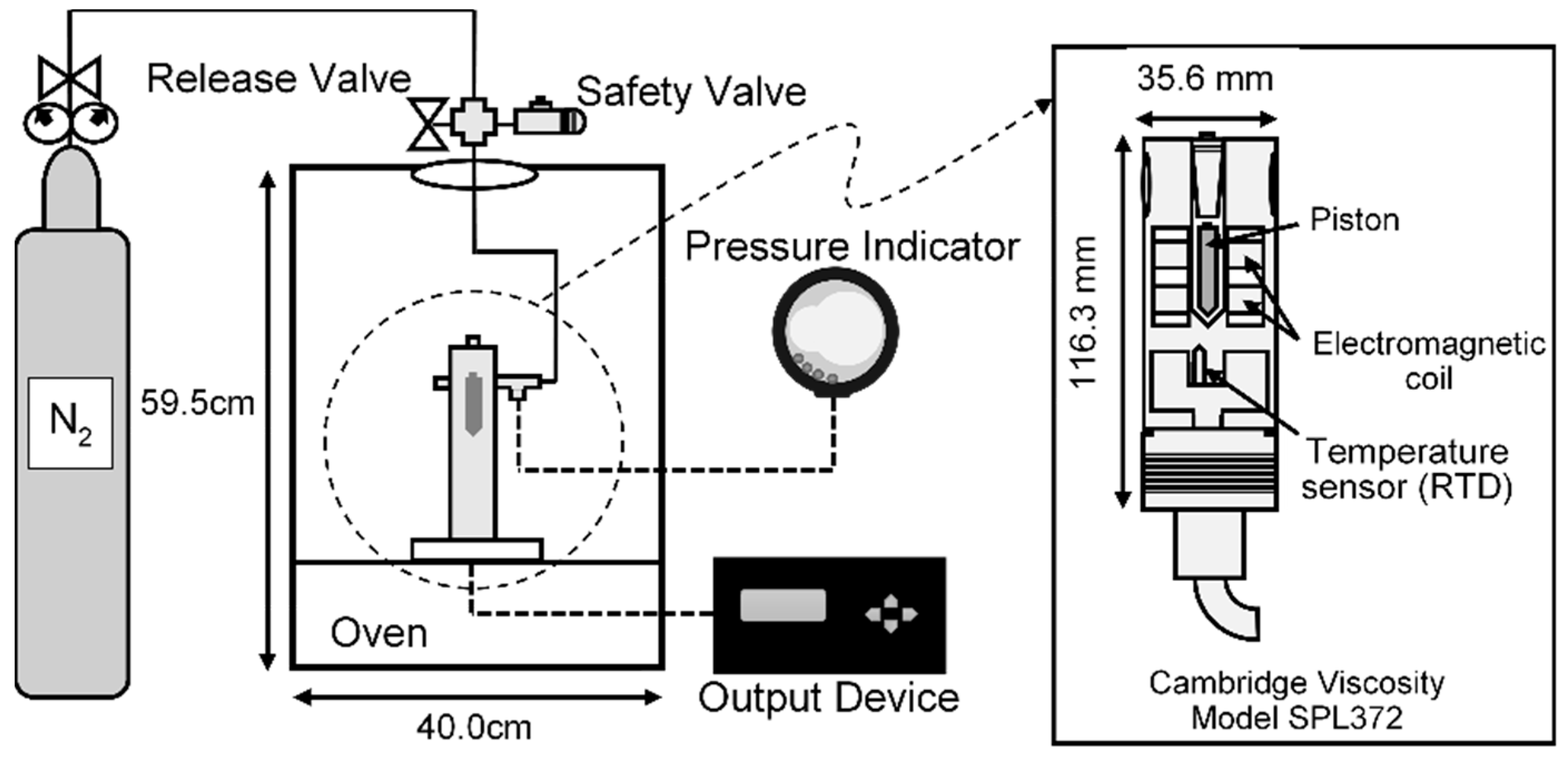
2.2.1. Measurement of Viscosity

The viscosity of the samples was measured at different temperatures and pressures using a high pressure and temperature Viscopro2000 Cambridge viscometer (Model SPL372, PAC, Houston, TX, USA) which is capable of measuring viscosity in the range of 0.2 mPas to 20,000 cP and at a maximum temperature and pressure of 190 °C and 7 MPa, respectively (see Figure 2). The operating principle is simply such that the instrument expresses the dynamic viscosity as a function of distance and time taken by the piston to move through the chamber. Temperature was measured with a platinum resistance temperature detector (RTD) mounted at the base of the chamber. About 10 mL of heavy oil sample was fed into the sample container and was pushed to the sensor. The system was heated to increase the temperature at intervals of 5 °C using the environment-controlled oven, and pressure was increased using nitrogen gas. The viscosity of sample X with 24% w/w asphaltene content was measured over a range of temperatures between 85 °C and 150 °C and a range of pressures between atmospheric pressure and 7 MPa. Similarly, sample Y (18.5% w/w asphaltene) was measured over the same range of pressure at temperatures between 70 °C and 120 °C and a range of pressures between atmospheric pressure and 7 MPa.

2.2.2. Viscosity Modeling

The viscosity data of the samples were fitted to the selected viscosity correlations. These include the following:

Power law function, Alade et al. [14]:

$$\mu =\nu T^{\theta }{P}^{\varnothing }$$

(1)

where $\mu$ (cP) is the viscosity at temperature T (°C) and pressure P (mPa). The constants v, θ, and ∅ are the system-specific empirical parameters.

Exponential function, Barus model [15,19]:

$$\frac{{\mu }_p}{{\mu }_{pr}}=\exp \left(\beta \Delta P\right)$$

(2)

where ${\mu }_{pr}$ is the viscosity of compressed bitumen at reference or atmospheric pressure ($P_r$) and ${\mu }_p$ is the viscosity of compressed bitumen at a particular pressure (P). The pressure difference $\Delta P=P-P_r$.

The pressure effectivity constant, $\beta$ (piezoviscous coefficient), is related to the temperature using an exponential Equation:

$$\beta =\exp \left(x_1+x_{2}T+x_3{T}^2\right)$$

where x₁, x₂, and x₃ are the constants.

Empirical correlations previously developed for the Cold Lake and Athabasca bitumen, Mehrotra and Svrcek [6,7]:

$$ln\left(\mu \right)=\exp \left(a_1+a_{2}lnT\right)+a_{3}P$$

(3)

$$lnln\left(\mu \right)=\left(a_1+a_{2}lnT\right)+a_{3}P$$

(4)

where $\mu$ (cP) is the viscosity at temperature T (°C) and pressure P (mPa). The constants a₁, a₂, and a₃ are the system-specific empirical parameters.

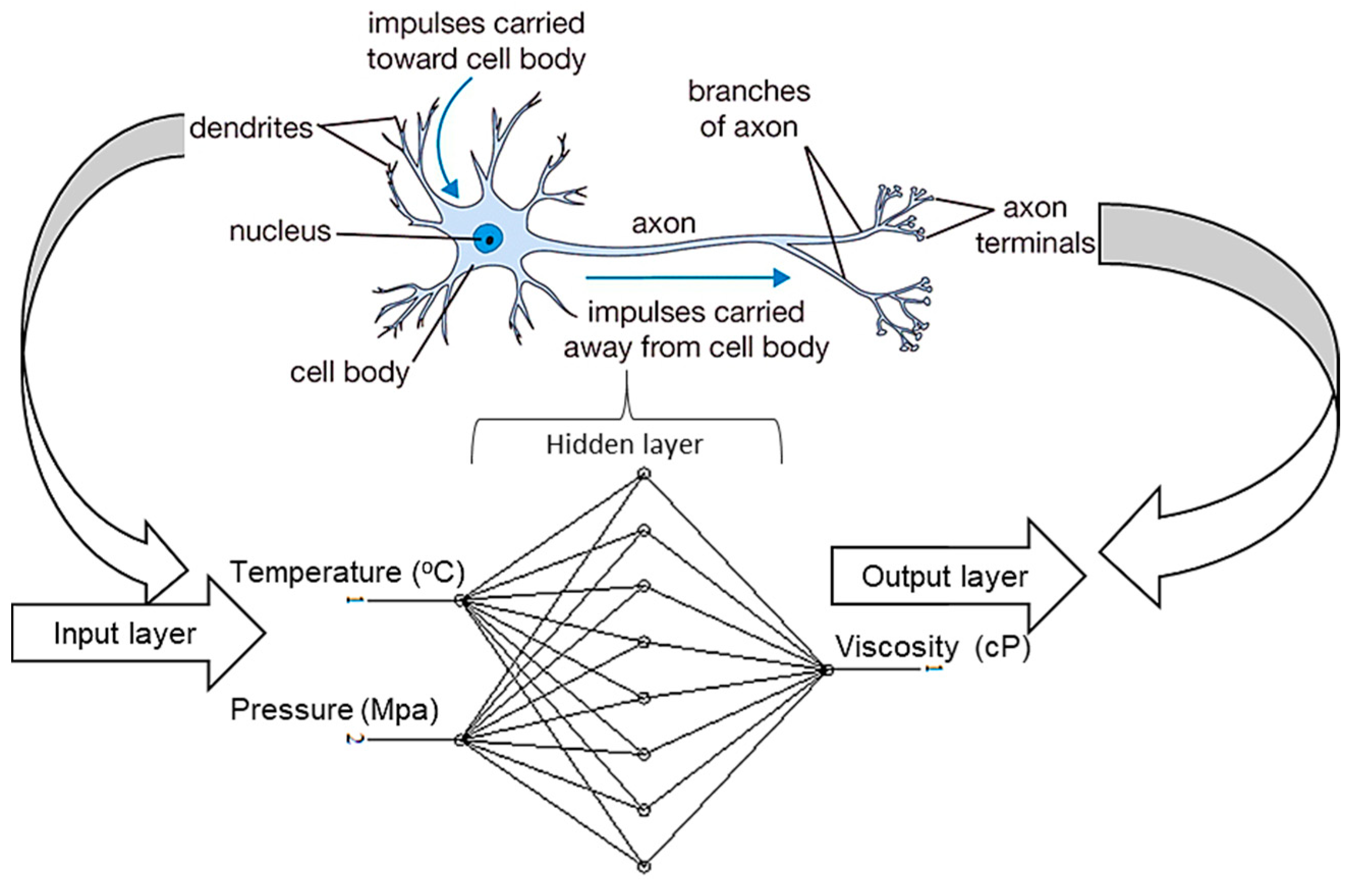
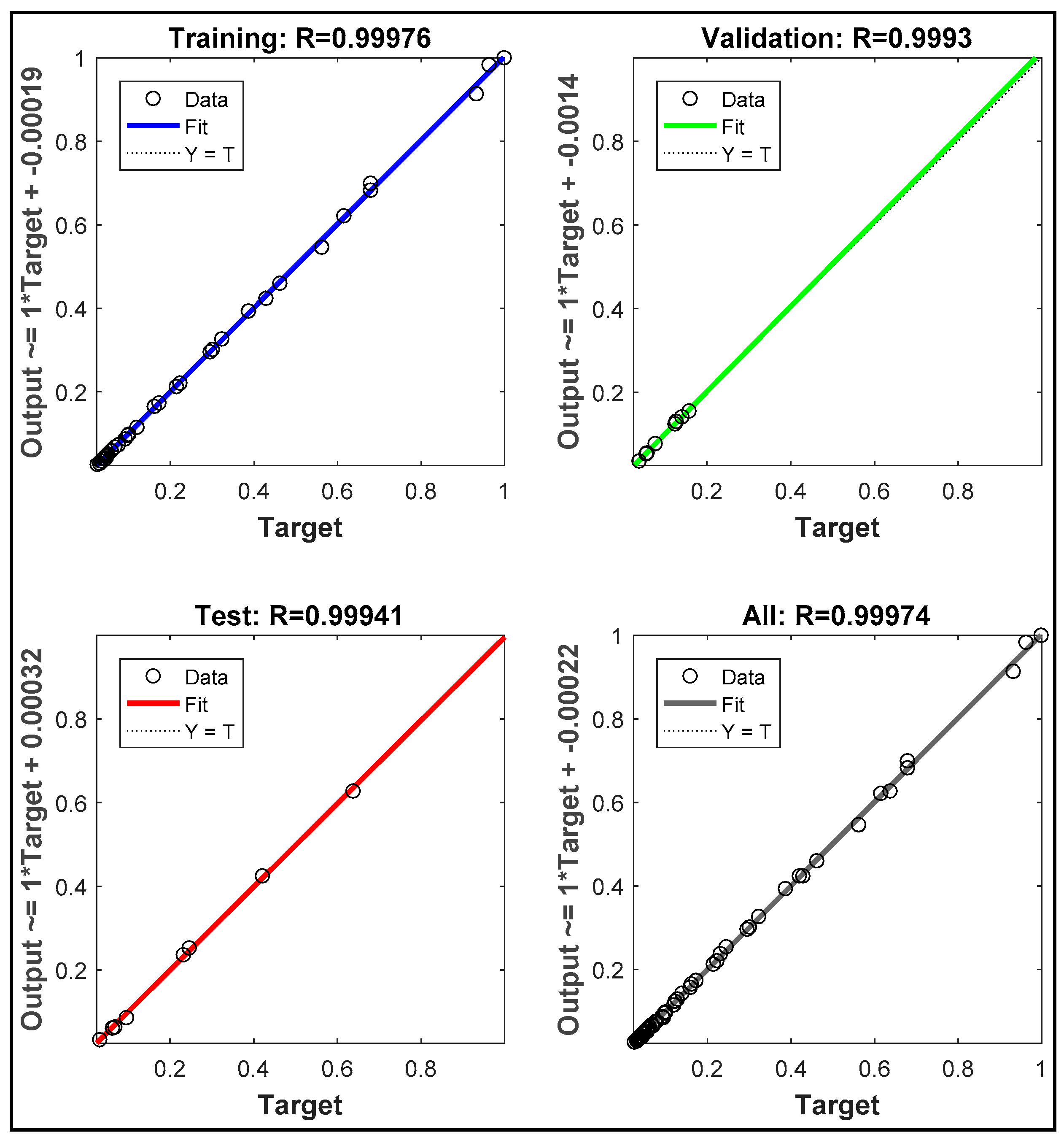
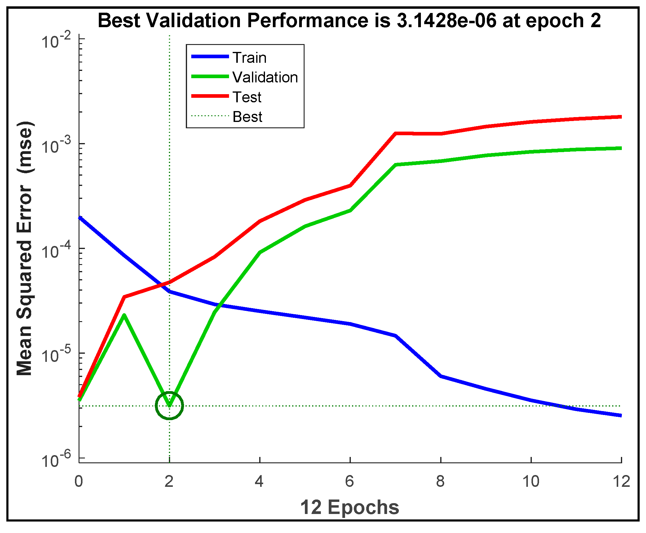
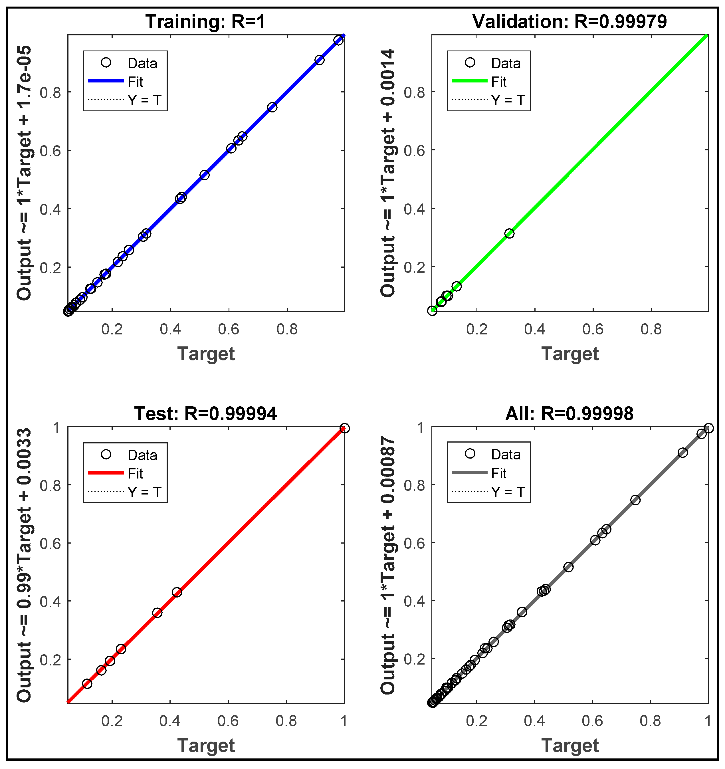
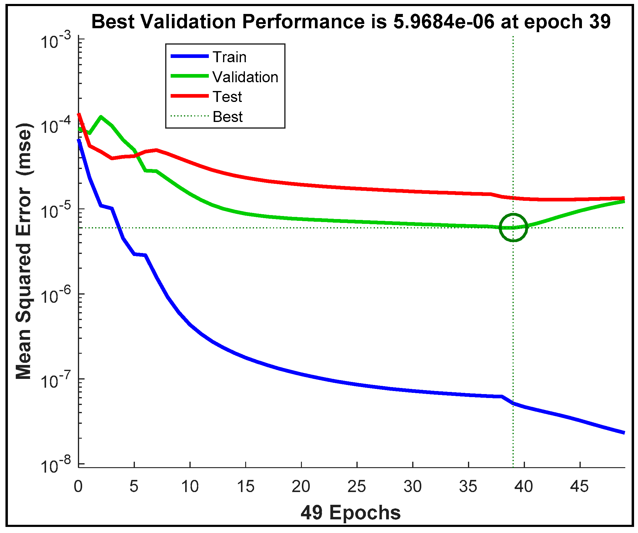
2.2.3. Development of the ANN Model

Essentially, in the ANN modeling, the neurons are connected via a connection link with an individual link having a weight that is multiplied with a transmitted signal in the network. The output of the network is determined by an activation function such as the hyperbolic tangent sigmoid function (tansig—Equation (5)), which is used for a nonlinear approximation.

$$tansig\left(n\right)=\frac{2}{1+e^{\left(-2n\right)}}-1$$

(5)

For n number of nodes, a simplified expression relating the input x_r to the output n_j is given in Equation (6).

$$n_j=f\left({\sum }_{r=1}^n{w}_{jr}{x}_r+b_j\right)$$

(6)

In the above expression, the weighting coefficient (w_jr) is applied to weaken or strengthen the input signals into each neuron. The biases (b_j) are activation thresholds added to the production of inputs and their particular weight coefficients. The transfer or activation function shows the net output of each neuron.

In this study, a multilayer feedforward neural network having temperature and pressure as the input variables and viscosity as the output variable was implemented using the Neural Network Toolbox in MATLAB (MATLAB 2016b, The Mathworks, Inc., Natick, MA‎, USA). The feedforward neural network utilizes the Levenberg–Marquardt (LM) back propagation-learning algorithm. This learning rule is an error minimization technique with backward error propagation (see Figure S1, Supplementary Materials). The architecture of the ANN model is presented in Figure S2, (see Supplementary Materials). For better performance, the input and output data were normalized between 0 and 1 using Equation (7). The primary application of the LM algorithm is in the least-squares curve-fitting problem where it has been primarily adopted as a standard technique. The Levenberg–Marquardt algorithm combines two minimization methods: the gradient descent method and the Gauss–Newton method. It has therefore been widely adopted as a training algorithm in the MATLAB ANN modeling due to its better performance in terms of accuracy and speed compared to other training algorithms:

$${\mu }_{norm}=\frac{{\mu }_{ac}}{{\mu }_{max}}$$

(7)

where µ_norm is the normalized value of viscosity, µ_ac is any value of the viscosity, and µ_max is the maximum value of the viscosity.

2.2.4. Statistical Error Analysis

The accuracy of the empirical models as well as the ANN was evaluated using the statistical parameters including the percentage deviation of error (%AAD), the root mean square error (RMSE), and the coefficient of determination (R²), Equations (8)–(10), respectively. The arithmetic average of the absolute values of the relative errors (%AAD) is an indication of the accuracy of the model. A low value of %AAD shows better correlation and lower error for the predicted values of viscosity. The RMSE is a measure of similar performance as indicated by the %AAD. The coefficient of determination (R²) is a measure of the precision of fit of the data. The maximum value of the R² is unity, and a high value indicates a high degree of agreement between the experimental and predicted viscosities.

$$\%AAD=\frac{100}{N_d}{\sum }_{i=1}^{N_d}\left|\frac{{\mu }_{exp}-{\mu }_{cal}}{{\mu }_{exp}}\right|$$

(8)

$$RMSE=\sqrt{\frac{1}{N_d}{\sum }_{i=1}{\left({\mu }_{exp}-{\mu }_{cal}\right)}^2}$$

(9)

$$R^2=1-\frac{{\sum }_{i=1}^{N_d}{\left({\mu }_{exp}-{\mu }_{cal}\right)}^2}{{\sum }_{i=1}^{N_d}{\left({\mu }_{mean}-{\mu }_{cal}\right)}^2}$$

(10)

3. Results and Discussion

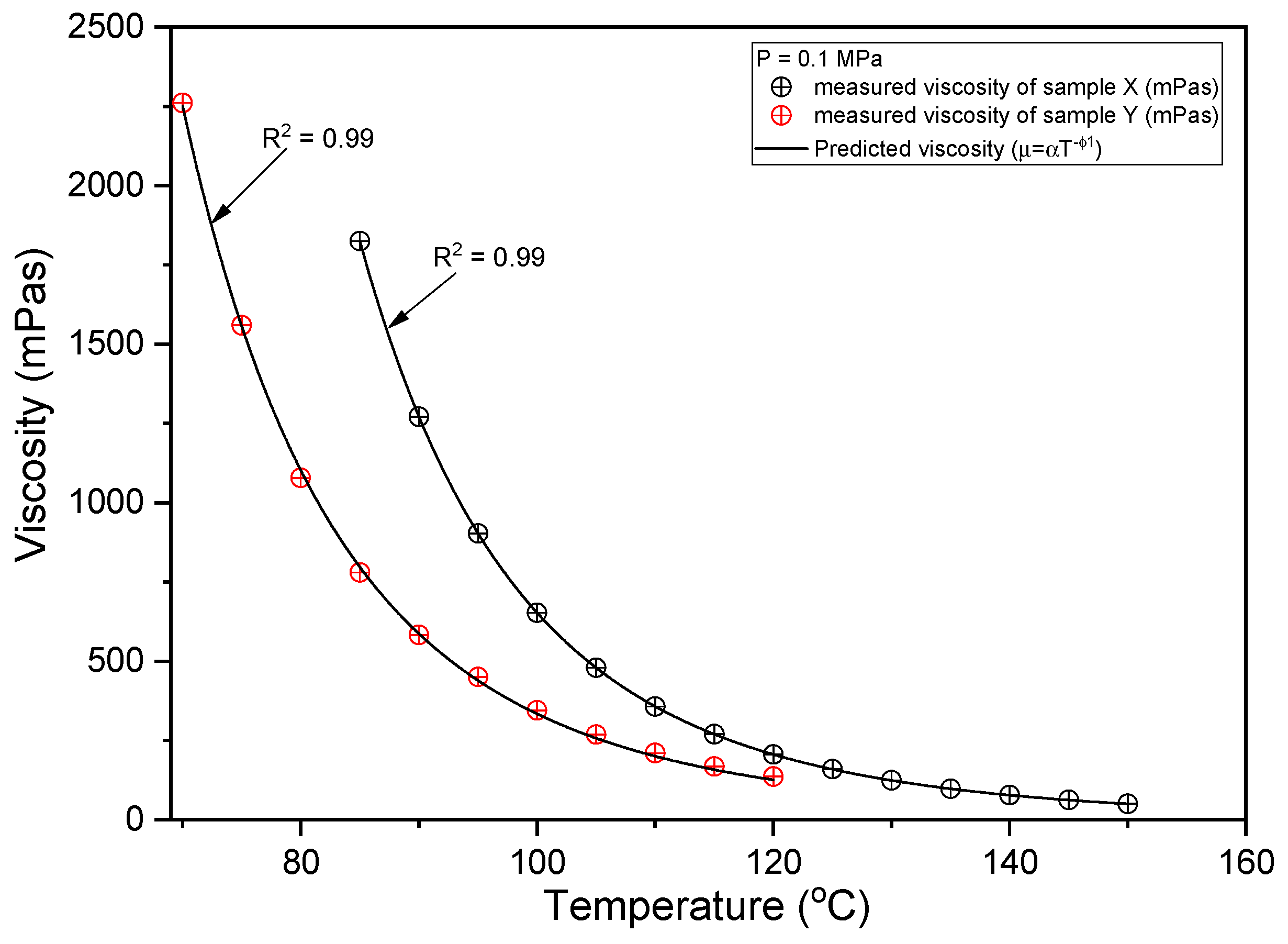
3.1. Viscosity Data of the Oil Samples

The viscosity data for the X and Y samples measured at different temperatures and pressures are presented in

Table 2. Correlation constants for the calculated viscosities of the oil samples.

Bitumen Samples	X			Y
	a1	a2	a3	a1	a2	a3
Mehrotra and Svrcek I	24.359	−3.797	0.047	22.074	−3.430	0.025
Mehrotra and Svrcek II	23.651	−3.678	0.008	21.759	−3.376	0.004
	v	θ	∅	v	θ	∅
Power law	3.47 × 1015	−6.326	0.074	2.3942 × 1013	−5.404	0.039
	x1	x2	x3	x1	x2	x3
Barus (1893)	−33.7638	0.55163	−0.00242	−0.72303	−0.04151	0.000116

. They show clearly that the viscosity decreases with increasing temperature at constant pressure, as expected. In other words, the viscosity increases with increasing pressure at constant temperature. However, the magnitude of increase in viscosity with pressure decreases slightly as the temperature increases. In addition, from the susceptibly due to the higher asphaltene content of sample X (see Table 1), it can be observed that the viscosity is higher than that of sample Y. Specifically, the viscosity of sample X, at 85 °C and atmospheric pressure (0.1 MPa), was observed as 1894 cP, and it increased to 2787 cP at 7 MPa. At 150 °C, the viscosity increased from 28 cP (at 0.1 MPa) to 33 cP at 7 MPa.

For sample Y, the viscosity at 70 °C and 0.1 MPa increased from 2260 cP to 3022 cP at 7 MPa. At 120 °C, the viscosity increased from 65 cP (0.1 MPa) to 71 mPas at 7 MPa. Furthermore, the viscosity temperature profiles (at atmospheric pressure) of the samples are compared in Figure 3. The figure ultimately shows that the data can be perfectly fitted (R² ≈ 1) using the power law function (μ = αT^β), where α and β are the empirical constants (sample X: α = 2.93 × 10¹⁵ and β = −6.33; sample Y: α = 1.68 × 10¹³ and β = −5.35).

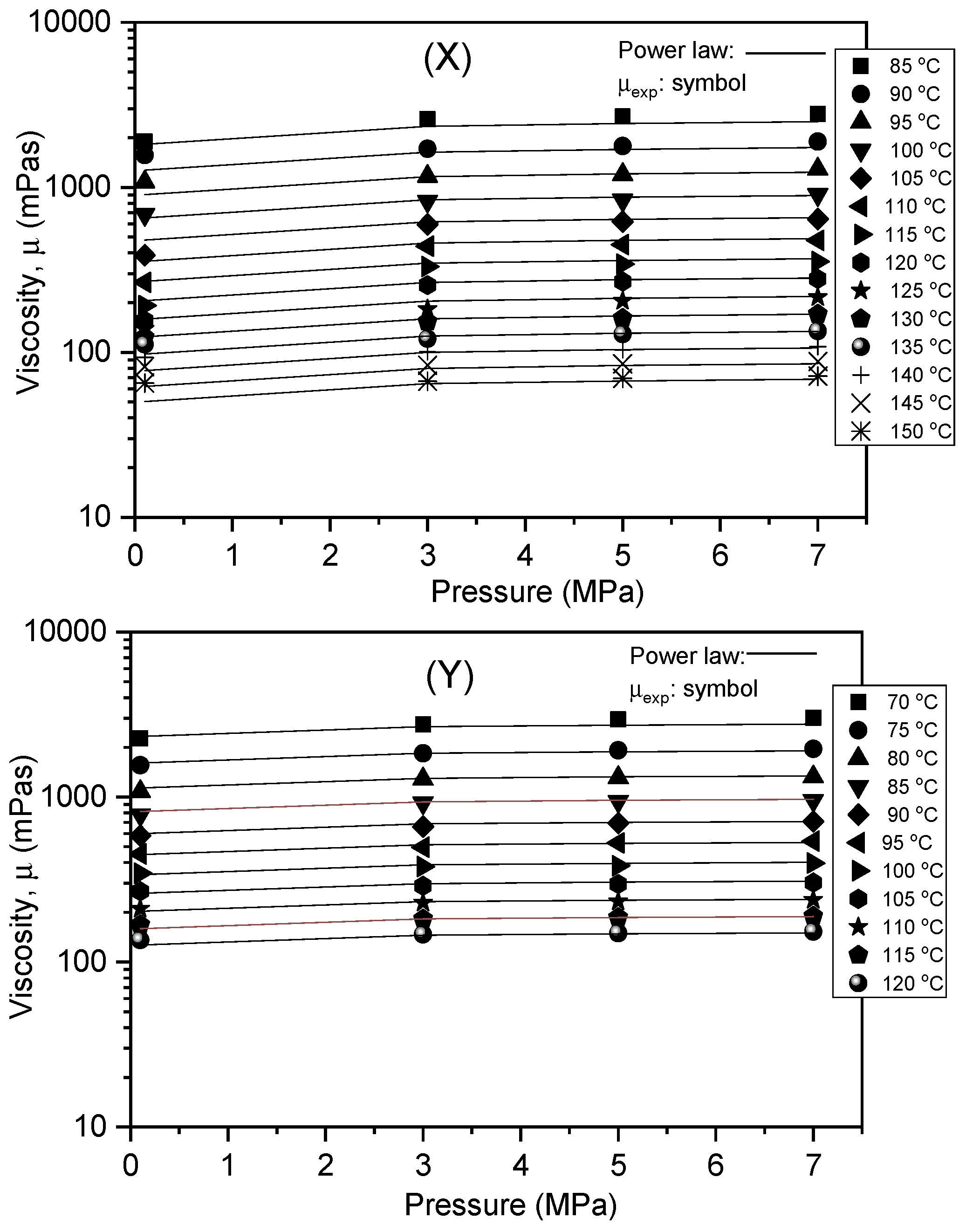
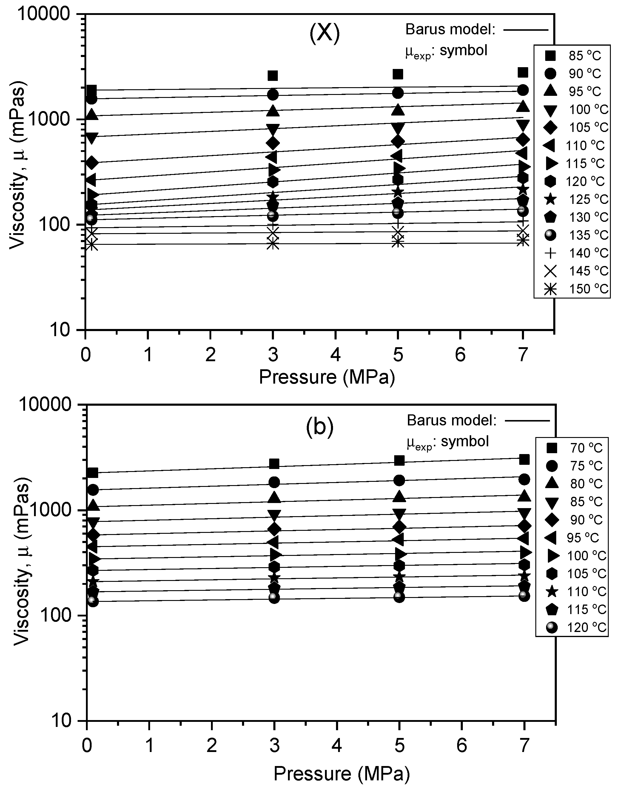
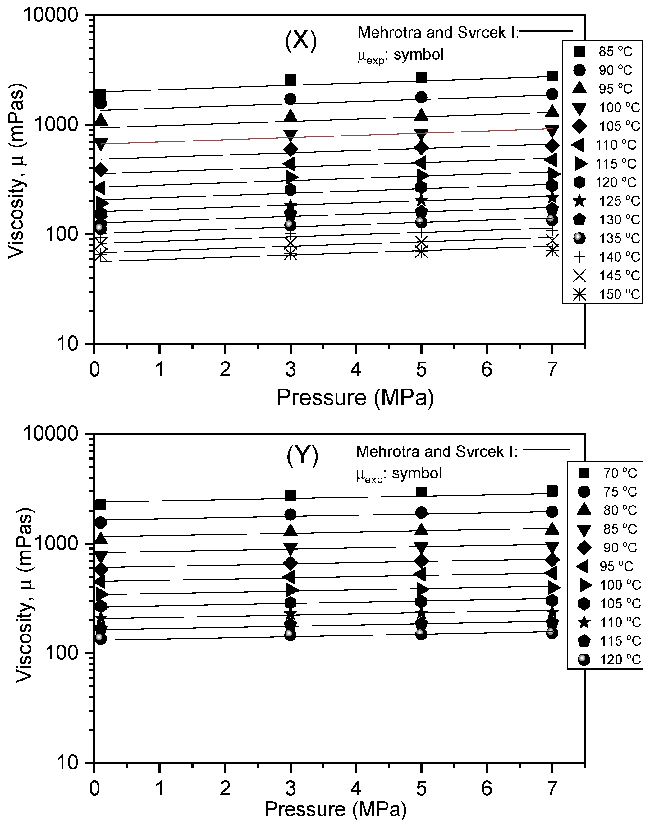
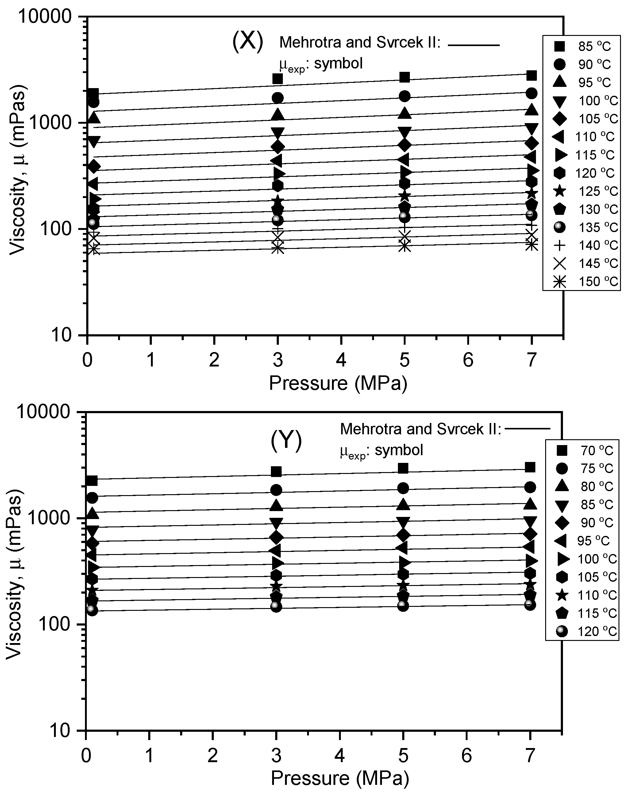
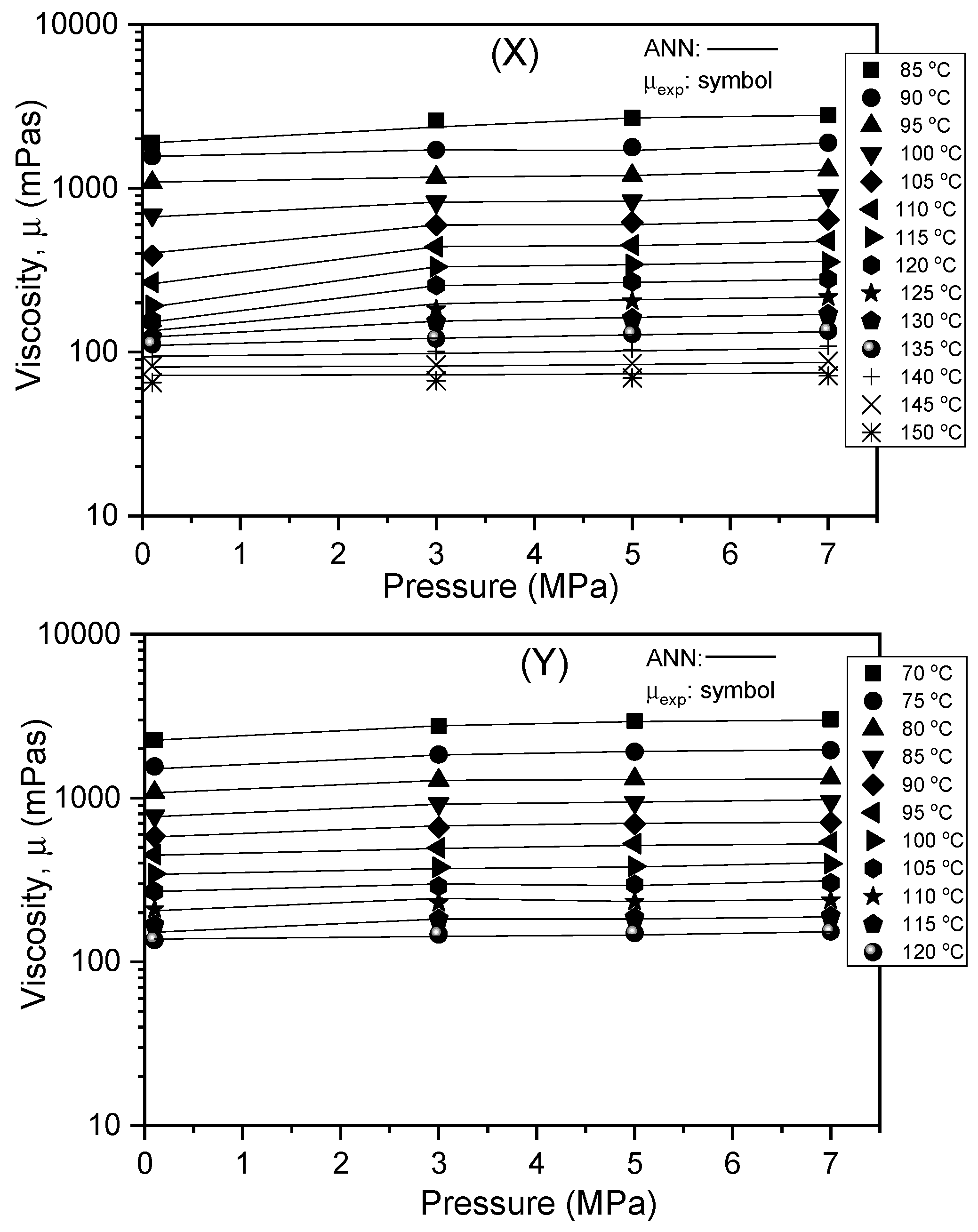
3.2. Viscosity–Temperature–Pressure (V-T-P) Modelling

The major objective of this study is to investigate the efficiency of available empirical models, namely, the power law (Equation (1)), the Barus exponential function (Equation (2)), and the three-parameter empirical functions (Equations (3) and (4)) compared to the artificial neural network (ANN) model in predicting viscosity of the samples.

The experimental and calculated viscosity data using Equations (1)–(4) and the ANN are presented in Figure 4, Figure 5, Figure 6, Figure 7 and Figure 8, respectively (the plotted viscosity values and the error values are available in the supplementary information: see Table S1a,b, Supplementary Materials, for the plotted viscosity values and Table S2a,b, Supplementary Materials, for the error values). The correlation constants for the models are presented in Table 2. The most popularly reported correlations for the viscosity–temperature–pressure relationships of bitumen are the three-parameter empirical Equations [6,7] developed for Canadian bitumen. Thus, the correlation constants for the three parameter models obtained in this work are compared with those that have been reported for Canadian bitumen.

From Table 2, for sample X (24.8% w/w asphaltene), the parameters a₁, a₂, and a₃ are 24.359, −3.797, and 0.047, respectively, using Equation (3) (Mehrotra and Svrcek, 1986). Then, using Equation (4), the values are 23.651, 3.678, and 0.008, respectively. The average absolute percent deviation (%AAD) absolute is 7.1712 and 7.078, for Equations (3) and (4), respectively. In the case of sample Y (18.5% w/w asphaltene), the values are relatively lower compared to sample X. These are 22.074, −3.430, and 0.025, respectively, using Equation (3); and from Equation (4), the values are 21.759, −3.376, and 0.004, respectively. The average absolute percent deviation (%AAD) = is 2.7183 and 1.8713, for Equations (3) and (4), respectively. As mentioned above, lower values of correlation constants were obtained for sample Y (which has lower viscosity) compared to sample X. With these observations, we can agree with the previous reports by Mehrotra and Svrcek [7] that the compression of lighter extra-heavy oil or bitumen yielded a slightly smaller increase in viscosity compared to the heavier one.

Moreover, the correlation constants reported above closely compared with the previous values reported for the Canadian bitumen samples [2,3,6,7]. Mehrotra and Svrcek [6], on the correlation of compressed Athabasca bitumen over a range of temperatures between 40 and 120 °C and pressures 0.1 MPa and 10 MPa, reported the parameters a₁, a₂, and a₃ as 23.4292, −3.6772, and 0.0345755, respectively, using Equation (3) (%AAD = 2.8). From Equation (4), the values were reported as 22.8515, −3.5784, and 0.005119, respectively, (%AAD = 2.8). Similarly, Mehrotra and Svrcek [7], on the correlation of compressed Cold Lake bitumen over the same ranges of temperatures and pressures, reported that the parameters a₁, a₂, and a₃ were 22.6437, −3.56121, and 0.028779, respectively, using Equation (3) (%AAD = 2.2). From Equation (4), the values were reported as 22.13520, −3.47381, and 0.004288, respectively, (%AAD = 2.1). In addition, the duo of Nourozieh et al. [2] and Kariznovi et al. [3] reported similar correlation constants obtained from their works on the viscosity of compressed Athabasca bitumen measured over a range of temperatures up to 200 °C and pressures up to 10 MPa. Using Equation (3), for three different bitumen samples, the parameters a₁ ranged between 23.94318 and 25.65193, a₂ ranged between −4.04208 and −3.76445, while a₃ ranged between 0.031101 and 0.040273 (%AAD = 8.4). From Equation (4), the values were between 22.92858 and 24.84525, −3.90450 and −3.59230, and 0.004704 and 0.007243, for a₁, a₂, and a₃, respectively (%AAD = 3.4–9.2).

Furthermore, the correlation constants obtained from the other models including the ANN are available in

Table 3. Comparison of statistical parameters for the correlations.

Model	Mehrotra and Svrcek I		Mehrotra and Svrcek II		Power Function		Barus Function		ANN Model
Bitumen Sample	X	Y	X	Y	X	Y	X	Y	X	Y
R2	0.9886	0.9937	0.9855	0.9942	0.9830	0.9943	0.9331	0.9968	0.9995	0.9999
RMSE	71.6074	60.1350	81.2810	57.7763	84.3289	57.3053	161.3737	44.5842	16.4611	5.3377
%AAD	7.1712	2.7183	7.0783	1.8713	7.5396	1.8898	7.6811	2.5827	2.4385	0.6609

. The statistical parameter to compare the accuracy of the correlations to predict the viscosity of the bitumen samples within the conditions of pressure and temperature operated are presented in Table 3. Most notably, compared to the other models, the ANN model gives the least error values calculated as %AAD of 2.4385 and 0.6609 for samples X and Y, respectively. From the other models, the values of %AAD range between 1.8713 and 7.1712. In addition, using the ANN, the values of RMSE were calculated as 16.4611 and 5.3377 for X and Y, respectively, while the values of RMSE calculated from other models range between 44.584 and 161.374. Similarly, the highest coefficient of determination, R² = 0.9995, was calculated for X and R² = 0.9999 for Y using the ANN compared to the other models.

For reference purposes, the ANN regression plots for sample X is presented in Figure 9; and as shown in Figure 10, the best validation performance is 3.1428 × 10⁻⁶. Similarly, for sample Y, the ANN regression plot is presented in Figure 11; and Figure 12 is the best validation performance (5.9684 × 10⁻⁶).

4. Conclusions

The viscosity data of two bitumen samples X and Y, with asphaltene contents 24.8% w/w and 18.6% w/w, respectively, were measured over a range of temperatures between 70 °C and 150 °C and a range of pressures between atmospheric pressure and 7 MPa. The viscosity data were fitted to empirical models including the three-parameter models developed for Canadian bitumen (Mehrotra and Svrcek, 1986 and 1987). The data were found to fit adequately to these models at acceptable levels of statistical indications. Moreover, compared to the empirical models, statistical analysis confirmed the superiority of the ANN approach for a better prediction of the viscosity data within the limit of conditions operated in this study.

References

1. Alade, O.S.; Sasaki, K.; Sugai, Y.; Ademodi, B.; Nakano, M. Bitumen emulsification using a hydrophilic polymeric surfactant: Performance evaluation in the presence of salinity. J. Pet. Sci. Eng. 2016, 138, 66–76. [Google Scholar] [CrossRef]
2. Nourozieh, H.; Kariznovi, M.; Abedi, J. Density and viscosity of Athabasca bitumen samples at temperatures up to 200 °C and pressures up to 10 MPa. SPE Reserv. Eval. Eng. 2015, 18, 375–386. [Google Scholar] [CrossRef]
3. Kariznovi, M.; Nourozieh, H.; Guan, J.G.; Abedi, J. Measurement and modelling of density and viscosity for mixtures of Athabasca bitumen and heavy n-alkane. Fuel 2013, 112, 83–95. [Google Scholar] [CrossRef]
4. Zirrahi, M.; Hassanzadeh, H.; Abedi, J. Prediction of bitumen and solvent mixture viscosity using thermodynamic perturbation theory. J. Can. Pet. Technol. 2014, 53, 48–54. [Google Scholar] [CrossRef]
5. Bryan, J.; Mirotchnik, K.; Kantzas, A. Viscosity Determination of Heavy Oil and Bitumen Using NMR Relaxometry. J. Can. Pet. Technol. 2003, 42, 29–34. [Google Scholar] [CrossRef]
6. Mehrotra, A.K.; Svrcek, W.Y. Viscosity of compressed Athabasca bitumen. Can. J. Chem. Eng. 1986, 64, 844–847. [Google Scholar] [CrossRef]
7. Mehrotra, A.K.; Svrcek, W.Y. Viscosity of compressed Cold Lake bitumen. Can. J. Chem. Eng. 1987, 65, 672–675. [Google Scholar] [CrossRef]
8. Puttagunta, V.R.; Singh, B.; Miadonye, A. Correlation of bitumen viscosity with temperature and pressure. Can. J. Chem. Eng. 1993, 71, 447–450. [Google Scholar] [CrossRef]
9. Xin, X.; Li, Y.; Yu, G.; Wang, W.; Zhang, Z.; Zhang, M.; Ke, W.; Kong, D.; Wu, K.; Chen, Z. Non-Newtonian Flow Characteristics of Heavy Oil in the Bohai Bay Oilfield: Experimental and Simulation Studies. Energies 2017, 10, 1698. [Google Scholar] [CrossRef]
10. Abukhalifeh, H.; Lohi, A.; Upreti, S.R. A Novel Technique to Determine Concentration-Dependent Solvent Dispersion in Vapex. Energies 2009, 2, 851–872. [Google Scholar] [CrossRef] [Green Version]
11. Chen, Z.; Li, X.; Yang, D. Quantification of Viscosity for Solvents−Heavy Oil/Bitumen Systems in the Presence of Water at High Pressures and Elevated Temperatures. Ind. Eng. Chem. Res. 2019, 58, 1044–1054. [Google Scholar] [CrossRef]
12. Eleyedath, A.; Swamy, K.A. Prediction of density and viscosity of bitumen. Pet. Sci. Technol. 2018, 36, 1779–1786. [Google Scholar] [CrossRef]
13. Radhakrishnan, V.; Chowdari, S.G.; Reddy, K.S.; Chattaraj, R. A predictive model for estimating the viscosity of short-term-aged bitumen. Road Mater. Pavement Des. 2018, 19, 605–623. [Google Scholar] [CrossRef]
14. Alade, O.S.; Ademodi, B.; Sasaki, K.; Sugai, Y.; Kumasaka, J.; Ogunlaja, A.S. Development of models to predict the viscosity of a compressed Nigerian bitumen and rheological property of its emulsions. J. Pet. Sci. Eng. 2016, 145, 711–722. [Google Scholar] [CrossRef]
15. Behzadfar, E.; Hatzikiriakos, S.G. Rheology of bitumen: Effects of temperature, pressure, CO2 concentration and shear rate. Fuel 2014, 116, 578–587. [Google Scholar] [CrossRef]
16. Martın-Alfonso, M.J.; Martinez-Boza, F.J.; Navarro, F.J.; Fernandez, M.; Crispulo, G. Pressure–temperature–viscosity relationship for heavy petroleum fractions. Fuel 2007, 86, 227–233. [Google Scholar] [CrossRef]
17. Appeldorn, J.K. A simplified viscosity-pressure-temperature equation. SAE Tech. Pap. 1963. [Google Scholar] [CrossRef]
18. Farobie, O.; Hasanah, N.; Matsumura, Y. Artificial neural network modelling to predict biodiesel production in supercritical methanol and ethanol using spiral reactor. Procedia Environ. Sci. 2015, 28, 214–223. [Google Scholar] [CrossRef]
19. Barus, S. Isothermals, isopiestics, and isometrics relatives to viscosity. Am. J. Sci. 1963, 45, 87–96. [Google Scholar] [CrossRef]
20. Sunphorka, S.; Chalermsinsuwan, B.; Piumsomboon, P. Artificial neural network model for the prediction of kinetic parameters of biomass pyrolysis from its constituents. Fuel 2017, 193, 142–158. [Google Scholar] [CrossRef]
21. Meng, X.; Jia, M.; Wang, T. Neural network prediction of biodiesel kinematic viscosity at 313 K. Fuel 2014, 121, 133–140. [Google Scholar] [CrossRef]
22. Deosarkar, M.P.; Sathe, V.S. Predicting effective viscosity of magnetite ore slurries by using artificial neural network. Powder Technol. 2012, 219, 264–270. [Google Scholar] [CrossRef]
23. Ramadhas, A.S.; Jayaraj, S.; Muraleedharan, C.; Padmakumari, K. Artificial neural networks used for the prediction of the cetane number of biodiesel. Renew. Energy 2006, 31, 2524–2533. [Google Scholar] [CrossRef]
24. Kalogirou, S.A. Artificial neural networks in renewable energy systems applications: A review. Renew. Sustain. Energy Rev. 2001, 5, 373–401. [Google Scholar] [CrossRef]
25. Hosseini, S.M.; Pierantozzi, M.; Moghadasi, J. Viscosities of some fatty acid esters and biodiesel fuels from a rough hardsphere-chain model and artificial neural network. Fuel 2019, 235, 1083–1091. [Google Scholar] [CrossRef]
26. Li, F.; Zhang, J.; Oko, E.; Wang, M. Modelling of a post-combustion CO2 capture process using neural networks. Fuel 2015, 151, 156–163. [Google Scholar] [CrossRef]
27. Betiku, E.; Omilakin, R.O.; Ajala, O.S.; Okeleye, A.A.; Taiwo, A.E.; Solomon, B.O. Mathematical modeling and process parameters optimization studies by artificial neural network and response surface methodology: A case of non-edible neem (Azadirachta indica) seed oil biodiesel synthesis. Energy 2014, 72, 266–273. [Google Scholar] [CrossRef]
28. Agwu, O.E.; Akpabio, J.U.; Alabi, S.B.; Dosunmu, A. Artificial Intelligence Techniques and their Applications in Drilling Fluid Engineering: A Review. J. Pet. Sci. Eng. 2018. [Google Scholar] [CrossRef]
29. Kiss, A.; Fruhwirth, K.R.; Leoben, M.; Pongratz, R.; Maier, R. Formation breakdown pressure prediction with artificial neural networks. In Proceedings of the SPE International Hydraulic Fracturing Technology Conference and Exhibition, Muscat, Oman, 16–18 October 2018. SPE-191391-18IHFT-MS. [Google Scholar]
30. Adeeyo, Y.A.; Saaid, M.I. Artificial Neural Network modeling of viscosity at bubblepoint pressure and dead oil viscosity of Nigerian crude oil. In Proceedings of the SPE NAICE Conference, Lagos, Nigeria, 31 July–2 August 2017. SPE-189142-MS. [Google Scholar]
31. Ebaga-Ololo, J.; Chon, B.H. Prediction of Polymer Flooding Performance with an Artificial Neural Network: A Two-Polymer-Slug Case. Energies 2017, 10, 844. [Google Scholar] [CrossRef]
32. Elkatatny, S.; Tariq, Z.; Mahmoud, M. Real time prediction of drilling fluid rheological properties using artificial neural networks visible mathematical model (white box). J. Pet. Sci. Eng. 2016, 146, 1202–1210. [Google Scholar] [CrossRef]
33. Ghaffarian, N.; Eslamloueyan, R.; Vaferi, B. Model identification for gas condensate reservoirs by using ANN method based on well test data. J. Pet. Sci. Eng. 2014. [Google Scholar] [CrossRef]
34. Li, X.; Miskimins, J.L.; Hoffman, B.T. A combined bottom-hole pressure calculation procedure using multiphase correlations and artificial neural network models. In Proceedings of the SPE Annual Technical Conference and Exhibition, Amsterdam, The Netherlands, 27–29 October 2014. SPE-170683-MS. [Google Scholar]
35. Al-Fattah, S.M.; Startzman, R.A. Predicting natural gas production using artificial neural network. In Proceedings of the SPE Hydrocarbon Economics and Evaluation Symposium, Dallas, TX, USA, 2–3 April 2001. SPE-68593. [Google Scholar]
36. Lopez, R.; Perez, J.R.; Dassori, C.G.; Ranson, A. Artificial Neural Networks Applied to the Operation of VGO Hydrotreaters. In Proceedings of the SPE Latin American and Caribbean Petroleum Engineering Conference, Buenos Aires, Argentina, 25–28 March 2001. SPE 69500. [Google Scholar]
37. Adebiyi, F.M.; Omode, A.A. Organic, Chemical and Elemental Characterization of Components of Nigerian Bituminous Sands Bitumen. Energy Sources Part A Recovery Util. Environ. Eff. 2007, 29, 669–676. [Google Scholar] [CrossRef]
Figure 1. A typical schematic of computational neuron adopted from a biological neuron (source: adapted from Farobie et al. [18]).
Energies 12 02390 g001
Figure 2. High-pressure high temperature viscometer set-up.
Energies 12 02390 g002
Figure 3. Viscosity of bitumen samples at different temperatures and atmospheric pressures.
Energies 12 02390 g003
Figure 4. Experimental and calculated viscosities using Equation (1).
Energies 12 02390 g004
Figure 5. Experimental and calculated viscosities using Equation (2).
Energies 12 02390 g005
Figure 6. Experimental and calculated viscosities using Equation (3).
Energies 12 02390 g006
Figure 7. Experimental and calculated viscosities using Equation (4).
Energies 12 02390 g007
Figure 8. Experimental and calculated viscosities using the ANN model.
Energies 12 02390 g008
Figure 9. Artificial neural Network (ANN) regression plots for sample X.
Energies 12 02390 g009
Figure 10. Best validation performance (for sample X).
Energies 12 02390 g010
Figure 11. Artificial neural network (ANN) regression plots for sample Y.
Energies 12 02390 g011
Figure 12. Best validation performance (for sample Y).
Energies 12 02390 g012