1. Introduction
Climate change is largely due to the relentless rise in carbon dioxide (CO
2) levels in the atmosphere since the Industrial Revolution, stemming from the world’s heavy reliance on fossil fuels. Global electricity generation amounted to 24,973 TWh in 2016 (38.4% from coal, 3.7% from oil and 23.2% from natural gas), while global CO
2 emissions from fuel combustion totalled 32,316 Mt [
1]. CO
2 emissions can be reduced on both the supply and demand sides through carbon capture and storage (CCS), increased use of renewable energy (RE) and energy efficiency enhancement. RE plays a central role in the transition to a low-carbon sustainable energy system; however, despite sharp cost reductions for solar photovoltaic (PV) and wind power, most renewables are still more expensive and less reliable than conventional fossil and nuclear energy in many parts of the world. On the other hand, CCS has been shown to be an integral part of any lowest-cost mitigation scenario with an increase in long-term global average temperature significantly less than 4 °C [
2]. CCS allows significant emissions reductions in power generation and industrial processes, and provides the foundation for negative emissions. Without CCS, the Paris Agreement commitments could not be met [
3].
Carbon-constrained energy planning (CCEP) is an established area of research with an effort to reduce climate change effects. Several early CCEP techniques were developed under the framework of carbon emissions pinch analysis (CEPA), which is an extension of conventional pinch analysis for heat and mass integration in the process industries to macro-scale applications such as regional and national electricity generation sectors. Tan and Foo [
4] presented a graphical procedure using composite curves to determine the optimal energy allocation that meets the specified energy demands and emissions limits, while minimising the use of zero-carbon energy sources. Their method was extended to consider other dimensions of sustainable energy systems, such as land availability, water consumption and electricity cost constraints. In addition to the development of an algebraic targeting approach to CCEP, Foo et al. [
5] addressed the problem of land-constrained energy planning for biofuel production. Tan et al. [
6] introduced a graphical targeting tool for analysing water footprint constraints on biofuel production systems. Bandyopadhyay and Desai [
7] proposed a pinch-based method to address the problem of cost optimal energy sector planning. Segregated planning for the allocation of energy sources to industry and transport subsectors was also addressed using an automated targeting approach [
8]. These pinch-based techniques are, however, limited to single-footprint or single-quality-index problems. Such a limitation can be overcome by using mathematical programming [
9], or by using the analytic hierarchy process (AHP) to compute an aggregate quality index [
10].
CEPA has been applied to electricity sectors in several countries. Crilly and Zhelev [
11] investigated Ireland’s electricity generation sector with forecasting and time-pinch adaptations to CEPA. Atkins et al. [
12] examined the implications of the 90% RE target on the generation mix and emissions levels for New Zealand in 2025. Walmsley et al. [
13] investigated the impacts of California reaching its 33% renewable electricity target by 2020 through generation cost analysis. The New Zealand transport sector was also analysed using a modified CEPA method [
14]. Apart from CEPA approaches, various mathematical programming models have been developed for energy planning. Bai and Wei [
15] presented a linear programming (LP) model to evaluate the effectiveness of possible CO
2 mitigation options for the electricity sector, using Taiwan as a case study. Mixed integer linear programming (MILP) with integer/binary decision variables is more commonly used. Hashim et al. [
16] formulated a MILP model for the problem of reducing CO
2 emissions from a power grid, and applied the model to an Ontario Power Generation fleet. Muis et al. [
17] developed a MILP model for the optimal planning of electricity generation schemes in Peninsular Malaysia. Koltsaklis et al. [
18] presented a spatial MILP model for the optimal long-term energy planning of the Greek power system. Chang [
19] presented a scenario-based MILP model for composite power system expansion planning for Taiwan, considering the influence of uncertain factors. Other variants and extensions of CCEP include the development of the composite table algorithm [
20] and a hybrid P-graph and Monte Carlo simulation approach [
21], and the incorporation of inoperability constraints [
22], uncertainties in learning rates and external factors (fuel and CO
2 prices) [
23], and multiple objectives (cost, water and land use minimisation) [
24].
For further emissions reductions, CCS options have been included in CCEP. Tan et al. [
25] presented a graphical pinch-based methodology for planning CCS retrofits in the power generation sector, aiming to determine the minimum extent of retrofitting required to meet the sectoral carbon footprint target. The need for additional power generation or efficiency improvements to compensate for energy losses from CCS retrofits is also considered. Their approach was extended by Ooi et al. [
26] to multi-period planning problems. Ooi and co-workers also developed extended automated targeting models to allow CO
2 load transfer between time intervals [
26], as well as discrete selection of power plants to be retrofitted [
27]. Concurrently, Bandyopadhyay and co-workers developed an algebraic pinch-based targeting technique for grid-wide CCS retrofit planning [
28] and an optimisation model for low-carbon power generation planning [
29]. The latter contribution overcame a limitation of an earlier study [
30], in which it was assumed that no existing power plants could be retrofitted for CCS. In addition, Chen et al. [
31] explored low-carbon technology roadmaps of China’s power sector. Ilyas et al. [
32] estimated the minimum CCS retrofitting and compensatory renewable power generation for the South Korean electricity sector using a pinch-based approach. Walmsley et al. [
33] combined CEPA and energy return on energy investment (EROI) analysis to investigate the feasibility of New Zealand’s reaching and maintaining a renewables electricity target above 90% through to 2050. Jia et al. [
34] presented a multi-dimensional pinch analysis of the power generation sector in China, considering carbon, water and land footprints as well as EROI and human risks. Almansoori and Betancourt-Torcat developed a steady-state optimisation model for the design of the United Arab Emirates’ power system [
35] and a multi-period model for the planning under uncertainty in the natural gas price [
36]. Other works on the use of optimisation models addressed economic impacts in achieving CO
2 emissions reduction targets [
37], parametric uncertainties in technological and cost coefficients [
38], uncertain future electricity demand [
39], and multistage generation expansion planning (GEP) with CCS [
40].
More recently, Lee [
41] developed a multi-period optimisation model for planning power plant retrofits with carbon capture (CC) technologies in the context of CCEP. This model considers variations in the performance and cost parameters to account for technological advances and allows more accurate planning results. Malkawi et al. [
42] evaluated Jordan’s energy options for electricity generation based on financial, technical, environmental, ecological, social, and risk assessment criteria using the AHP. Different scenarios were considered and sensitivity analyses performed to investigate the effect of varying criteria weights. Lim et al. [
43] applied CEPA and its extensions to a country-level analysis of the United Arab Emirates’ goal of reducing carbon emissions from its electricity sector, also considering EROI and water consumption. Two scenarios for achieving the carbon emission target were analysed, with discussion on the climate–energy–water nexus. For economy-wide analysis, Tan et al. [
44] proposed a hybrid approach combining CEPA with input–output analysis. The latter describes supply chain linkages in an economic system and allows life cycle-based carbon footprints of the sectors to be computed and used in CEPA, instead of direct CO
2 emissions considered in conventional CEPA methodology. A recent review by Foo and Tan [
45] discusses the development of process integration (PI) techniques for various emission and environmental footprint problems. Another recent review by Manan et al. [
46] summarises the PI methodologies for CO
2 emissions reduction, focusing on the development of pinch-based graphical, algebraic and numerical tools for supply side, demand-side and end-of-pipe management. DeCarolis et al. [
47] formalised best practice for energy system optimisation modelling, and outlined a set of principles and modelling steps to guide model-based analysis. There have been various optimisation techniques and algorithms proposed for optimal green energy planning [
48], as well as different models for GEP optimisation with RE integration [
49].
Table 1 provides an overview of previous CCEP studies based on PI approaches. Apart from these techniques, MARKAL [
50], Switch [
51], NEMS [
52] and ERCOM [
53] are among the most well-known energy systems models in the literature. The importance of incorporating planetary boundaries in designing sustainable energy mixes has been highlighted by Algunaibet et al. [
54].
From the literature review, it is obvious that CCEP is an important approach for meeting energy demand and footprint limits. Moreover, CCS has been recognised as a key technology to achieve the energy and environmental goals. In most previous studies on CCEP involving CCS, power plants are grouped by fuel and CCS retrofitting is treated as a lumped single option without considering the selection of CC technologies. Furthermore, CCS retrofits were considered to only reduce the power output because of the additional energy consumption of CC processes, such as the separation of CO
2 from the flue gas and then from the sorbent in the case of post-combustion capture. However, different CC technologies have different suitability, performance and implications; some options using an auxiliary boiler and steam turbine can even increase the plant’s power output. Allowing for detailed technical parameters of various CC technologies and selecting the most suitable ones for power plants can thus be an important part of CCS retrofit planning and have an impact on the results. In this paper, a new mathematical programming model is developed for multi-footprint energy sector planning with deployment of CCS and renewables. The generic formulation considers a portfolio of different CCS options for each individual generation unit of fossil fuel power plants and employs the Integrated Environmental Control Model (IECM) [
55] to assess the performance and costs of different types of generation units before and after CCS retrofitting. Simulation results from the IECM are then used as input data in the planning model for detailed and comprehensive analysis. In the following sections, a formal problem statement is given first. The mathematical model is presented next. A case study is then used to illustrate the proposed approach. Finally, conclusions and prospects for future work are given at the end of the paper.
3. Model Formulation
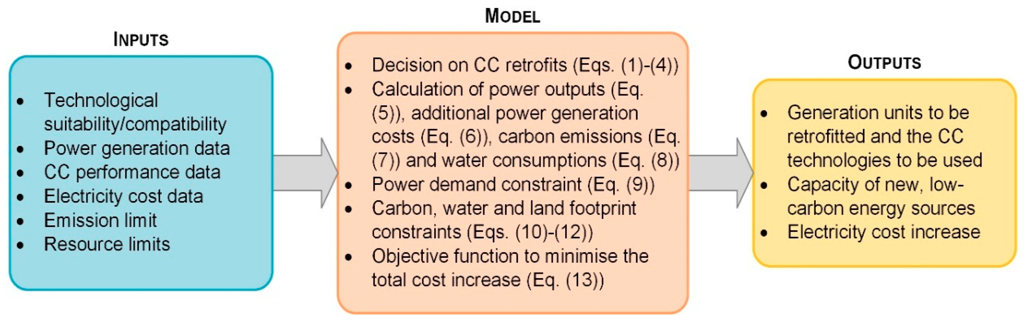
In this work, a mathematical model is developed for optimal deployment of CC technologies and renewables under multiple footprint constraints. The model requires data for power generation, CC performance and electricity cost. With these input data, the model is able to determine the strategy that minimises the cost increase due to CC retrofits and new, low-carbon power plants, while satisfying the specified emission and resource limits. The formulation is presented below. The notation used is given in the Nomenclature (see
Appendix A).
Equations (1)–(4) deal with the selection of CC technologies for thermal power plants and generation units. Equation (1) states that only one CC technology can be selected for each power plant to be retrofitted. Equation (2) defines the forbidden (
Mpk = 0) and allowable (
Mpk = 1) matches considering the compatibility between specific power generation and CC technologies. Equation (3) ensures that the selection made for plant
p applies to all its units
j ∈
Jp. In addition, if none of the units in plant
p is to be retrofitted using technology
k (
. ), no such selection should be made at the plant level (
ypk = 0). This is given in Equation (4).
The power generation of unit
j after plant retrofits and the corresponding increase in electricity cost are given by Equations (5) and (6), respectively. Please note that if unit
j is not retrofitted (
), the energy output will remain at the baseline level (
qj =
GjCFjTRj) with no additional cost (
xj = 0).
On the other hand, the carbon emissions and water consumption of unit
j are calculated using Equations (7) and (8), respectively. Similarly, these two equations give the results of retrofitting or the baseline carbon emission/water consumption levels (if unit
j is unmodified). It should also be noted that the footprints and levelised costs of electricity in Equations (6)–(8) are based on gross generation.
Equation (9) dictates that the energy demand should be satisfied. If the existing mix of energy sources cannot satisfy the demand, new power plants would be needed. Please note that the last two terms on the left-hand side of Equation (9) represent power generation from existing and additional low-carbon energy sources.
Equations (10) and (11) impose carbon and water footprint constraints on power generation. In both constraints, the first term on the left-hand side gives the contribution of thermal power plants (after retrofits), while the next two terms give those of the existing and new low-carbon power plants.
In addition, Equation (12) imposes a land footprint constraint on power generation from new, low-carbon plants.
The objective function is to minimise the total cost increase, which consists of the additional cost incurred by CC retrofits and the cost of power generation using new, low-carbon energy sources, as given in Equation (13).
Equations (1)–(13) constitute a MILP model, for which global optimality can be guaranteed without major computational difficulties.
Figure 1 summarises the model structure and the overall approach. It is worth noting that the model can be adapted and allows additional, case-specific constraints to be added, as discussed later in the Case Study.
In the next section, a case study of Taiwan is presented to illustrate the proposed approach. The corresponding model is implemented and solved in GAMS [
56] on a Core i7-7500U, 2.70 GHz processor, utilising CPLEX as the MILP solver. Solutions were found with negligible processing time (less than 1 CPU s) for all scenarios.
4. Case Study
This case study considers medium-term planning of Taiwan’s electricity sector for 2025, which is an initial checkpoint in Taiwan’s energy transition. By the end of 2017, the total installed capacity in Taiwan was 49.8 GW; the gross power generation in 2017 was 270.3 TWh [
57]. Thermal power plants using coal, oil and natural gas accounted for 73.8% of the total installed capacity and 85.9% of the total power generation.
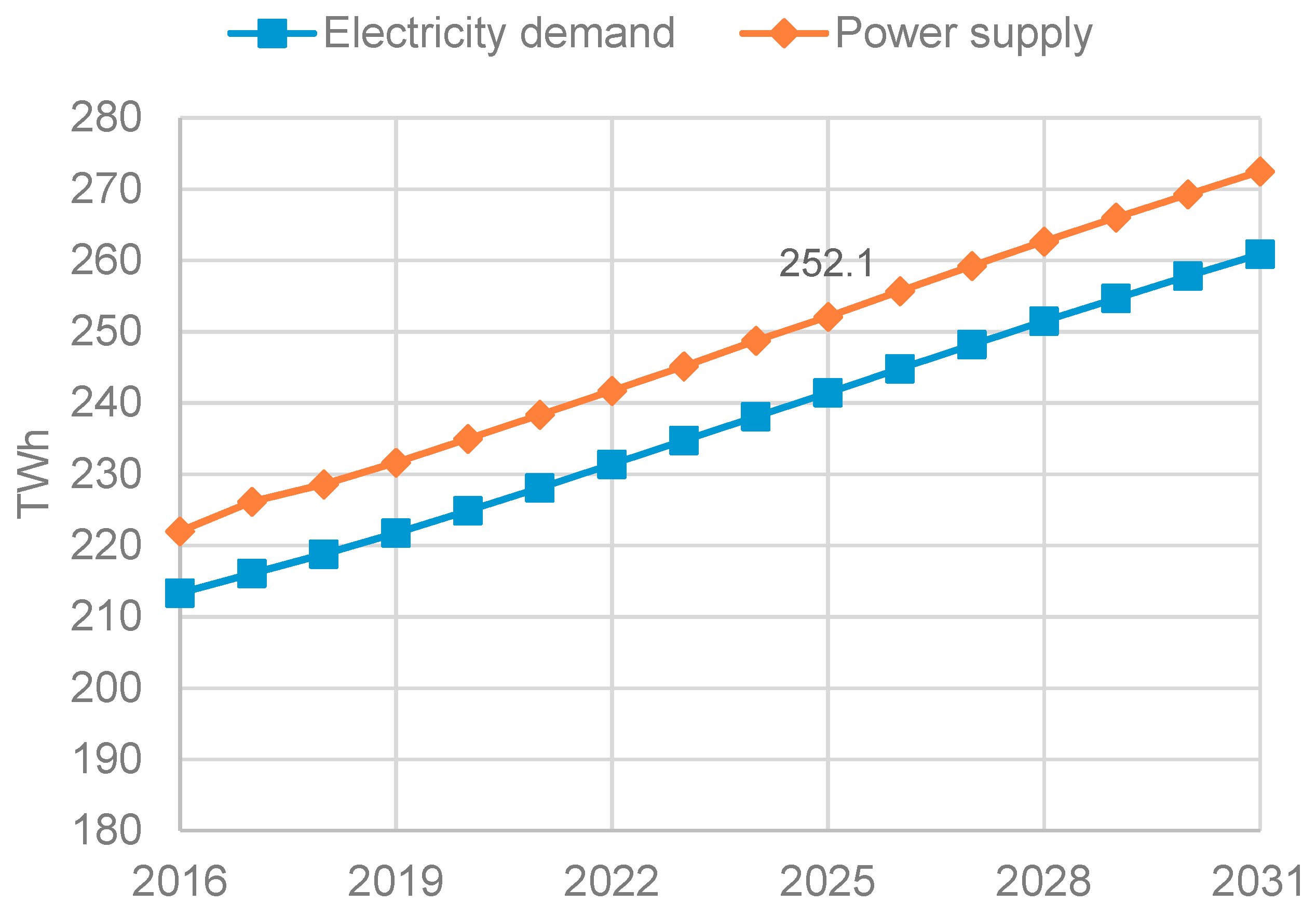
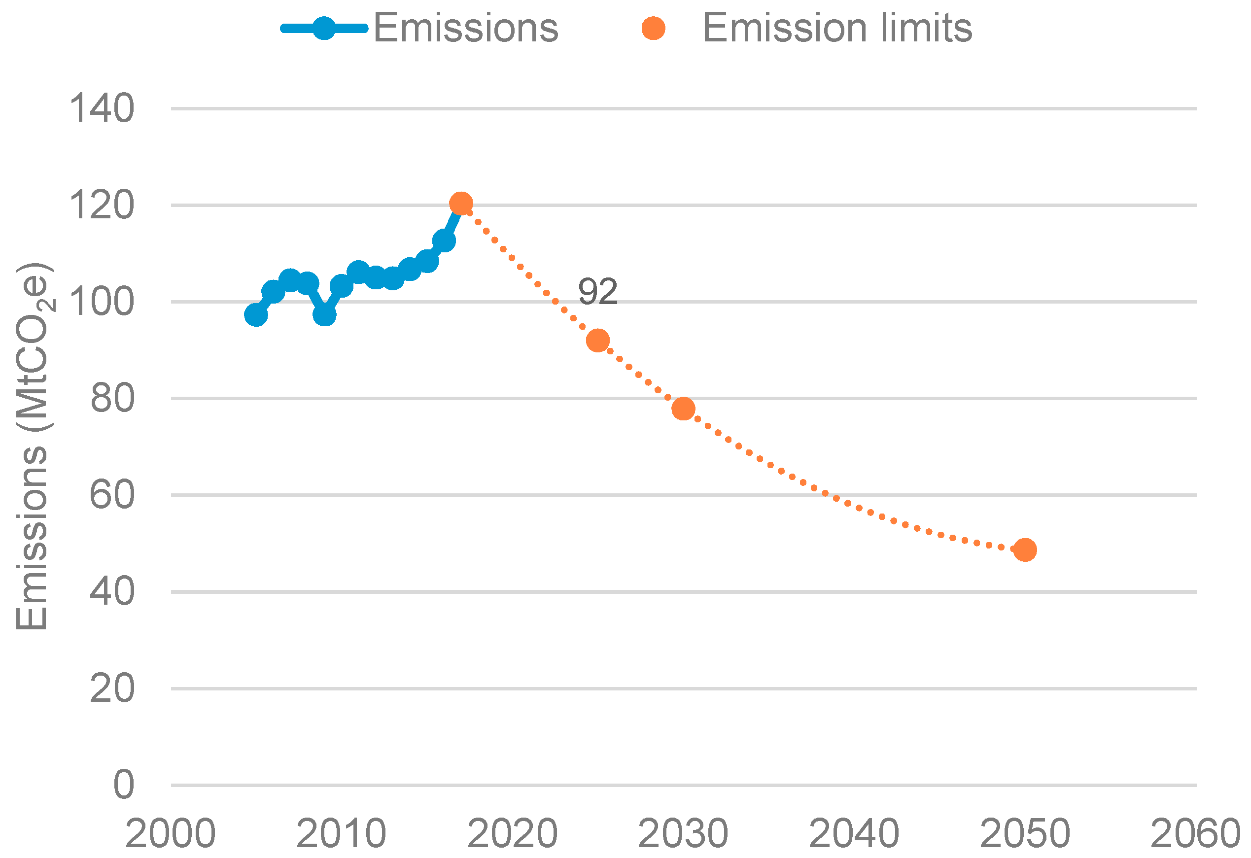
Figure 2 shows the 2017–2031 load forecast provided by the Taiwan Power Company (Taipower). With the growing demand for electricity, the required power supply is expected to increase at an average annual rate of 1.4%. This implies a concurrent increase in carbon emissions in the business-as-usual (BAU) scenario. In response to climate change, a long-term national goal has been set for Taiwan to reduce greenhouse gas (GHG) emissions to no more than 50% of the 2005 level by 2050. The government also aims to meet an economy-wide target of reducing GHG emissions by 50% from the BAU level, or by 20% from the 2005 level, by 2030. These targets are assumed in this work to apply directly to the electricity sector. Using historical data, the sectoral carbon emissions in 2005 are calculated to be 97.3 Mt (= 0.555 kgCO
2e/kWh [
58] × 175.3 TWh [
59]). The emissions limits for 2030 and 2050 are thus determined to be 77.8 (= 97.3 × 80%) and 48.6 (= 97.3 × 50%) MtCO
2e, respectively. Assuming a quadratic emissions reduction trajectory from the 2017 level, as shown in
Figure 3, the emissions limit for 2025 is estimated at 92 MtCO
2e.
Table 2 shows the baseline energy mix in 2025, based on Taipower’s long-term power development plan [
60]. The capacity factors are determined from Taipower’s 2013–2017 statistical data [
59] or taken from NREL estimates (for small hydro, offshore wind and geothermal) [
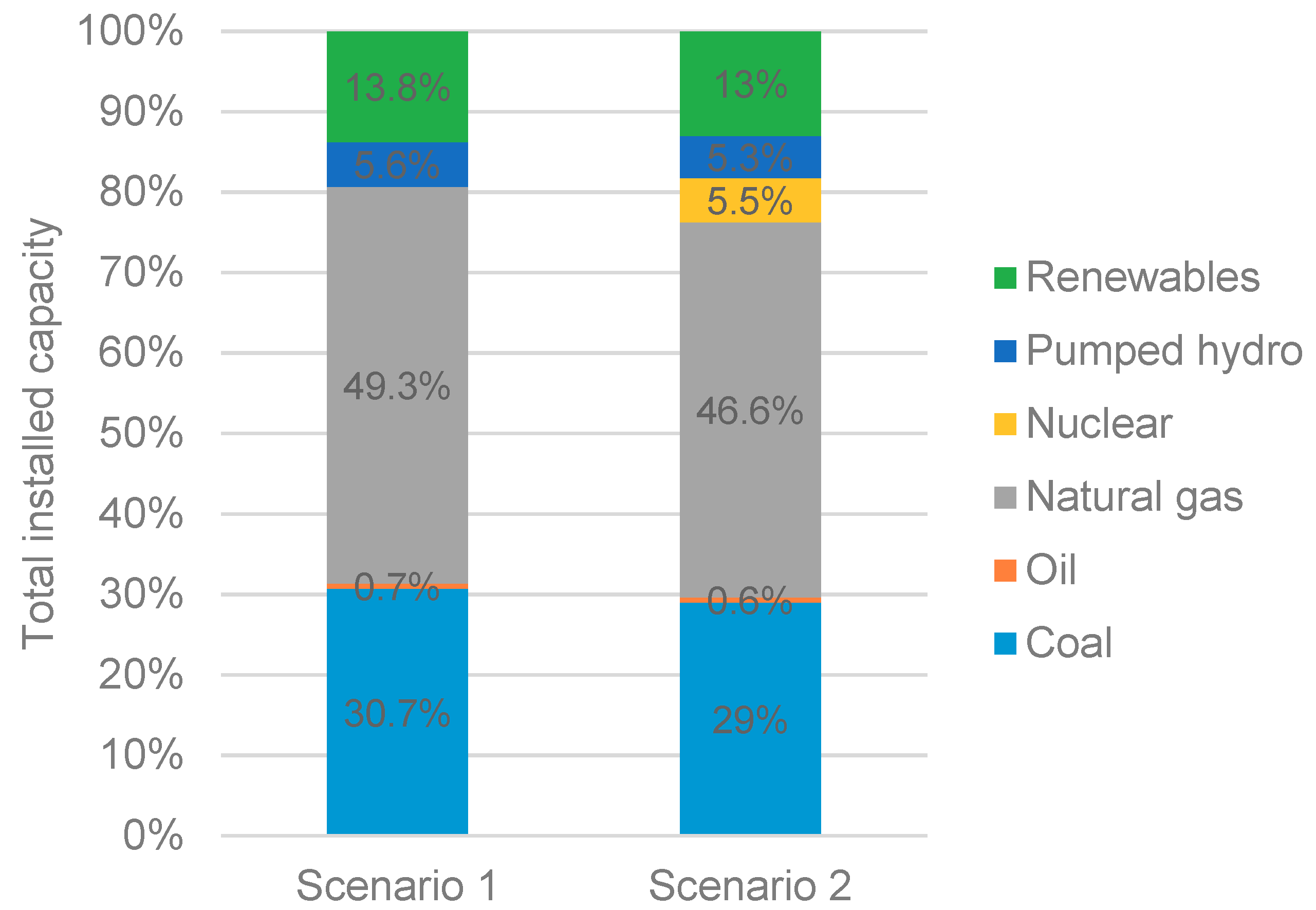
61]. Given the controversy over nuclear power, two scenarios (with and without the use of the fourth nuclear power plant) are considered in this case study.
Figure 4 shows that in both scenarios, thermal power plants using coal, oil and natural gas comprise more than 75% of the total installed capacity. This indicates the need for CCS and the expansion of RE in order for the electricity sector to meet the emissions limit (92 MtCO
2e) and the required power supply of 252.1 TWh (see
Figure 2) in 2025. Please note that the load forecast in
Figure 2 does not include pumping energy, which is about 2% of the power supply [
59]. Therefore, the overall energy demand to be satisfied in 2025 is 257.1 (= 252.1 × 1.02) TWh.
4.1. Plant Simulation
Table 3 lists the thermal power plants and generation units in the 2025 energy mix. Please note that SPPs are small power plants on offshore islands, where all the generators are oil-fired (with installed capacities ranging from 0.3 to 11 MW) and are lumped into a single unit, SPPO. Similarly, IPPs consist of nine private power plants, where coal-fired and gas-fired generation units are lumped into IPPC and IPPG, respectively. In this case study, only Taipower’s large generation units (excluding SPPs and IPPs) are considered for CCS, except HTC3, HTC4 and HTG3–HTG5, which are due to be decommissioned in 2026–2027. The CC options are post-combustion technologies that are relatively mature and suitable for existing power plants in Taiwan, including amine, ammonia (NH
3) and membrane systems [
62]. Oxy-fuel combustion and chemical (calcium) looping systems are excluded because these technologies are more suited to new power plants than existing ones. For amine and ammonia systems, there is the option of adding an auxiliary gas boiler to generate low-pressure steam for sorbent regeneration. An auxiliary steam turbine can then be used in conjunction with the gas boiler to generate additional power and/or low-pressure steam.
Table 4 shows the compatibility of the CC technologies with the thermal power plants. The membrane system requires a high concentration of CO
2 in the flue gas, and is therefore not suitable for gas-fired plants.
All the candidate plants for CCS were simulated using the IECM [
62] to assess their performance before and after the retrofit. Firstly, the plant type and the technologies for combustion/post-combustion controls and water and solids management were chosen according to the actual equipment of the plant. Next, the capacity factor and ambient conditions (temperature, pressure and humidity) were set for the overall plant. The installed capacity and turbine/boiler type were also entered, while the other parameters for the performance were calculated by default. Fuel properties (higher heating value and composition) and costs were then specified according to Taipower’s purchasing information. In addition, the ash properties of the coal (oxide content) also needed to be specified. The ash content determines the resistivity of the ash, and hence the specific collection area of the cold-side electrostatic precipitator.
Simulation results of the power generation units before CCS can be verified by comparing the IECM outputs with the actual performance. As an example,
Table S1 in the Supplementary Materials shows the comparison for unit TC1. It can be seen that the IECM provides accurate performance assessment, despite the discrepancy in the LCOE. Such a difference is due to the use of default capital and operating cost data in the IECM. For the simulation of retrofitted power plants, the CC system is selected on the plant design screen and configured on the corresponding “config” screen [
62].
Table S2 shows, as an example, the results of CC for unit TC1. In comparison to the baseline plant, the retrofitted plant (using an amine, ammonia or membrane system) can have an 86–90% reduction in carbon emissions, with a 14–36% reduction in net power generation and a 40–80% increase in the total cost. Adding an auxiliary gas boiler can reduce the power loss; furthermore, combining the gas boiler with a steam turbine can even increase the power output from the baseline level. However, using the auxiliary gas boiler and steam turbine results in additional carbon emissions (hence less emissions reduction) and a further increase in the total cost. It should be noted that, although not exactly accurate, the cost estimates of the IECM give correct relative costs of electricity, and are thus useful for planning Taiwan’s energy sector in 2025. The parameters obtained from IECM simulations for the case study are given in
Tables S3–S11 in the Supplementary Materials. Please note that the levelised costs of electricity from thermal power generation units are calculated based on costs in 2016. The parameters for low-carbon energy sources are given in
Table S12.
4.2. Planning Constraints
Apart from the energy demand and emissions limit discussed in
Section 4.1, there are also limits on water consumption, gas consumption and RE expansion. For water resource management, Taipower has set a water use target of no more than the average water consumption over the previous three years for its thermal power plants. In this case, Equation (11) is rewritten as Equation (14), where the water consumption limit for 2025 is set to the 2015–2017 average of 10.948 Mt [
63].
According to the Energy Transition White Paper [
64], the natural gas supply in Taiwan is expected to reach 32.7 Mt/y by 2025, of which about 80% can be used for power generation. Therefore, the gas consumption limit for 2025 is set to 26.16 (= 32.7 × 0.8) Mt. Equation (15) imposes this constraint on the thermal power plants.
where the gas consumption of unit
j is given by Equation (16).
Table 5 shows the government’s current targets for RE development [
65]. Instead of the land footprint constraint in Equation (12), this case study considers the capacity constraint on RE expansion, as given in Equation (17).
where the limit to the additional capacity of renewables is calculated by subtracting the baseline capacity (in
Table 2) from the target value.
4.3. Results and Discussion
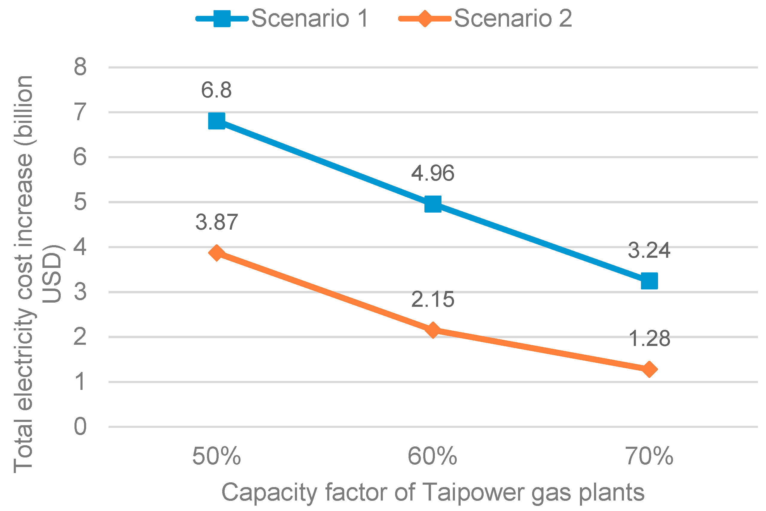
Two scenarios are considered in this case study to examine the role of nuclear power in the energy mix. In both scenarios, the effect of increasing the capacity factor of Taipower gas-fired plants (from 50% to 60% and to 70%) is further analysed. This represents a recent change of the gas-fired power plants from being load-following plants to being more like baseload plants.
Table 6 shows the baseline installed capacity, power generation and carbon emissions for the individual cases. It can be seen that in scenario 1 or 2, when the gas plant capacity factor is low (i.e., 50%), the baseline energy mix is incapable of meeting the energy demand of 257.1 TWh. At the same time, the baseline emissions exceed the emissions limit of 92 Mt in all the cases. Therefore, not only will CCS be necessary, but additional power generation from renewables or auxiliary steam turbines may also be required. The objective of the planning is to identify the optimal strategy that minimises the additional cost to the electricity sector.
Solving the MILP model for this case study (Equation (13) subject to Equations (1)–(10) and (14)–(17)) with the input data in
Table 2,
Table 3,
Table 4 and
Table 5 and
Table S3–S12 yields the results in
Table 7. The model involves 871 constraints and 859 variables (including 553 binaries), and is solved in 0.2–0.5 CPU s. Overall, the increase in electricity cost (from the baseline) decreases as the gas plant capacity factor increases, as shown in
Figure 5, and the use of nuclear energy reduces the additional costs. In scenario 1, increasing the power output from the gas plants reduces the need for CCS and additional power generation capacity. In other words, less capacity of thermal power plants is retrofitted, fewer auxiliary steam turbines are used, and less additional RE is required. The same is observed in scenario 2 when the gas plants operate at capacity factors of 50% and 60%. However, the capacity of thermal power plants for CCS is significantly increased when the gas plant capacity factor increases to 70%, although there is no need for auxiliary steam turbines or additional RE.
Table 8 shows the retrofitted power generation units and the selected CC technologies in each case. It can be seen that coal-fired generation units are prime targets for CCS, except in the last case, where most of the retrofitted units are gas-fired. In addition, the FG
+ amine system is the most selected because it has higher energy output ratios and is less expensive for gas-fired units.
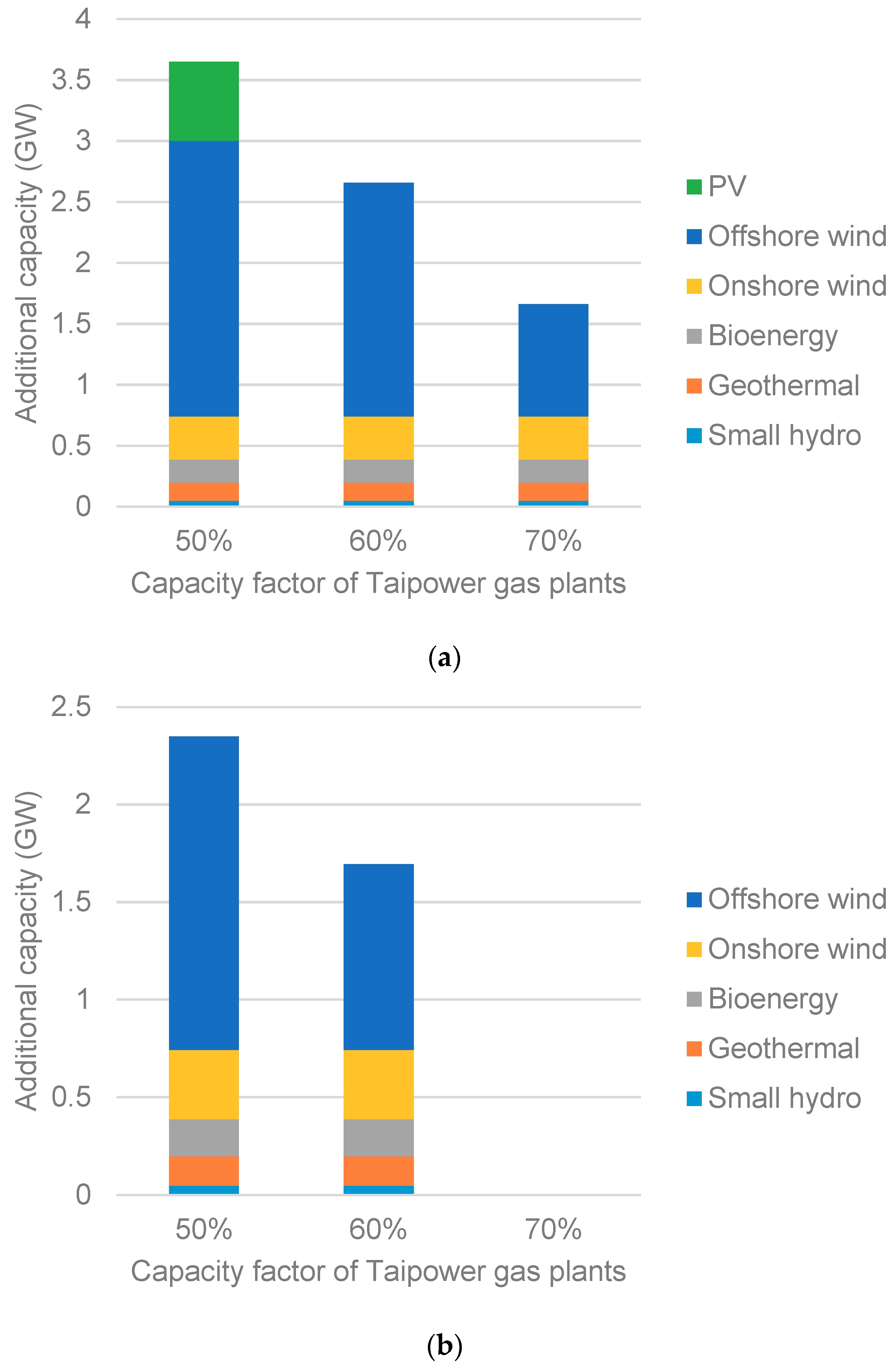
Figure 6a,b shows the additional RE capacities for scenarios 1 and 2, respectively. It appears that the sources with lower costs or higher capacity factors (i.e., small hydro, geothermal, bioenergy and onshore wind) are preferred, while additional PV is only required when all the others have reached their capacity limits. However, offshore wind has the largest share (> 55%) of the RE expansion.
In addition, the results demonstrate the role of nuclear power as an economical low-carbon option in energy transition. The use of nuclear energy reduces the need for additional power generation capacity from renewables in 2025, thus relieving the pressure to achieve ambitious RE targets in the medium term. This might seem to delay the deployment of renewables, but is actually to buy time for RE technologies to be deployed progressively in the long term, without major impacts on grid stability and electricity cost. With similar effects, increasing the capacity factor of load-following (i.e., gas-fired) power plants reduces the operating reserve, and hence grid flexibility, while causing difficulties in maintenance scheduling. Therefore, the preferred strategy would be to use nuclear energy with gas-fired plants operating at optimised capacity factors. It should be noted that there is no direct comparison between the results for scenarios 1 and 2, because of the different baseline conditions. However, the total levelised annual cost of nuclear power generation can be estimated to be 0.68 billion USD (= 2.7 × 10
6 kW × 8760 h × 0.901 × 0.032 USD/kWh), which is less than the difference in the resulting electricity cost increase between scenarios 1 and 2 (see
Figure 5). This indicates the economic benefit of nuclear energy in this specific case. As is the case for all energy technologies, nuclear power has its pros and cons, which would imply the incorporation of further environmental indicators in the planning for a sustainable energy mix.


