Article

Forecast Horizon and Solar Variability Influences on the Performances of Multiscale Hybrid Forecast Model

EA 4935 LaRGE, Laboratoire de Recherche en Géosciences et Énergies, Université des Antilles, 97170 Pointe-á-Pitre, France
*
Author to whom correspondence should be addressed.
Energies 2019, 12(12), 2264; https://doi.org/10.3390/en12122264
Submission received: 14 May 2019 / Revised: 2 June 2019 / Accepted: 3 June 2019 / Published: 13 June 2019
(This article belongs to the Section A2: Solar Energy and Photovoltaic Systems)

Abstract

:
The tropical insular region is characterized by a large diversity of microclimates and land/sea contrasts, creating a challenging solar forecasting. Therefore, it is necessary to develop and use performant and robustness forecasting techniques. This paper examines the predictive performance of a novel solar forecasting approach, the multiscale hybrid forecast model (MHFM), as a function of several parameters. The MHFM model is a technique recently used for irradiance forecasting based on a hybrid autoregressive (AR) and neural network (NN) model combined with multiscale decomposition methods. This technique presents a relevant performance for 1 h ahead global horizontal irradiance forecast. The goal of this work is to highlight the strength and limits of this model by assessing the influence of different parameters from a metric error analysis. This study illustrates modeling process performance as a function of daily insolation conditions and testifies the influence of learning data and test data time scales. Several forecast horizon strategies and their influence on the MHFM performance were investigated. With the best strategy, a rRMSE value from 4.43 % to 10.24 % was obtained for forecast horizons from 5 min to 6 h. The analysis of intra-day solar resource variability showed that the best performance of MHFM was obtained for clear sky days with a rRMSE of 2.91 % and worst for cloudy sky days with a rRMSE of 6.73 % . These works constitute an additional analysis in agreement with the literature about influence of daily insolation conditions and horizons time scales on modeling process.

1. Introduction

Solar forecasts are essential for grid-connected solar photovoltaics (PV) as penetration increases. The electrical output from solar resources is a major issue, particularly for islands with non-interconnected electrical network. Moreover, the frequent cloud formation with a diversity of solar microclimates leads to a challenging solar forecasting. Better solar forecasting tools contribute to improving the integration of this energy in the electric network. There is a rich literature on forecasting techniques (see [1,2,3] for a comprehensive review): methods using mathematical formalism of times series, numerical weather prediction (NWP) model and weather satellite imagery. According to the horizon, some of these methods are more effective compared to others [4]. Methods using mathematical formalism of time series show relevant predictive performance for horizons lower than one day (short time scales: from few minutes to few hours) such as connectionist models (artificial neural network) and more particularly the Multi-Layer Perceptron (MLP), which is the most often used artificial neural network architecture [5,6]. Some works in the literature demonstrate the solar forecasting performance using a combination of neural network (NN) model and other techniques: neural network mixed with wavelet [7], neural network mixed with neighboring meteorological sensors [8], and multiple parameters neural network model [9]. Reference models based on the family of ARMA (autoregressive moving average) and STARMA (spatiotemporal autoregressive moving average) also show a relevant predictive performance of solar radiation for short time horizons (e.g., [10,11,12,13,14]). In [15], a combination of autoregressive (AR) and neural network (NN) models is presented taking advantage of the unique strength of AR and NN models in linear and nonlinear modeling. In the preceding work [16], we investigated a hybrid forecast model using AR and MLP neural network models including multiscale decomposition methods (MD): wavelet decomposition methodology (WD) [17], empirical mode decomposition (EMD) [18], and ensemble empirical mode decomposition (EEMD) [19]. A multiscale hybrid forecast model (MHFM) is proposed, thus combining these three techniques (AR, NN and MD) for the first time in the literature. This new model has been successfully applied for solar radiation forecasting, demonstrating robustness and efficiency for a 1 h solar forecasting horizon particularly with wavelet decomposition method. In this present work, we investigated the forecast influence of strategies for short time scales horizons (from 5 min to 6 h) on the MHFM modeling process by testing the integration of different multiscale decomposition methods. Moreover, we analyzed the MHFM performance as a function of daily insolation conditions.
In the literature, the performance of several forecasting models is investigated as a function of forecast horizons [14,20,21,22,23,24], but for only one horizon strategy process. In this paper, for the first time in the literature, we present the forecasting performance of a model as a function of two horizon strategies on the modeling process and as a function of daily clearness index classification. For the solar radiation classification, several methods are proposed in the literature based on unsupervised clustering methods such as k-means [13,25], Ward’s method [26], best information criterion [27] or, recently, Fuzzy c-means method [28]. Fuzzy c-means method was used here. This method has shown relevant results previously [28]. Each class of typical day is defined by a variation of global solar radiation rate. For each class, the forecasting model is performed and the error is quantified. Moreover, this work presents a supplementary statistical analysis on the level of variability of daily solar radiation profiles, particularly ramp rates. Some authors have proposed a characterization and definition of ramp rates as the instantaneous differences in power output separated by the timescale of interest, normalized by the timescale (e.g., Equation (1) in Johnson et al. (2012) [29]). Others have looked at the magnitude and duration of ramps using assumed tolerances (minimum time offset from previous ramp and minimum magnitude) for defining individual ramps (e.g., Figure 1 in Hansen et al. (2010) [30]). The study presented here was based on the works of Lave et al. (2015) [31] who characterized local high-frequency solar variability and its impact to distribution. To categorize typical days as a function of their variability, the amplitude of fluctuations for different time scales was studied from the parameters presented in [31,32]. The goal of this work was to bring a statistical analysis on the scalability of predictive MHFM model performance as a function of the time scales of training data and test data, the process of calculating forecast horizons, and the daily variability of irradiance.
The paper is organized as follows: In Section 2, the data pre-processing and the processes and methods used in this work are presented. The results are described in Section 3. Several points indicate an influence on the models predictive performance. Section 4 examines and discusses the presented results. Finally, we conclude in Section 5.

2. Material and Methods

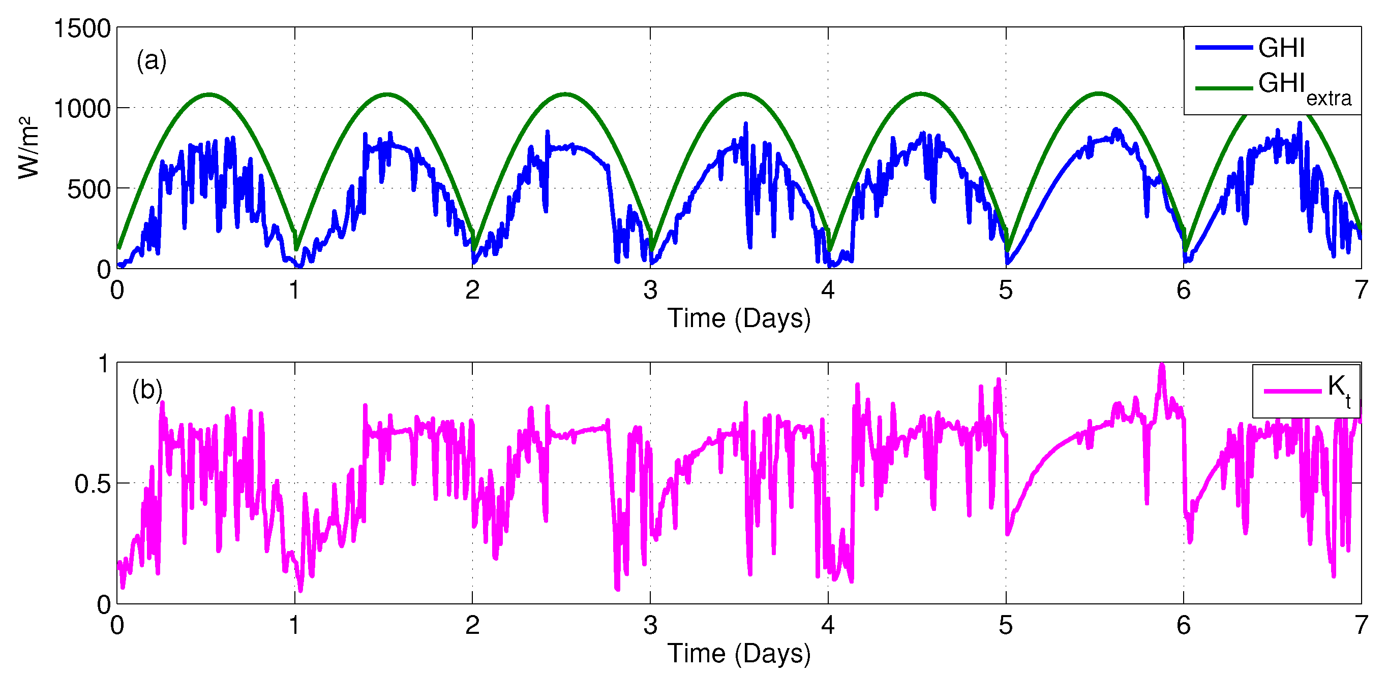
2.1. Data Pre-Processing

The global solar radiation measurements were collected at Petit-canal Gros-Cap ( 16 23 N latitude and 61 24 W longitude), along the cliffs of Guadeloupe island. The dataset includes measurements at 1 Hz with a CM22 from Kipp and Zonen pyranometer (type SP Lite) whose response time is less than a second. For this study, a sampled database was used at 5, 10, 15, 30 min and 1 h of the solar global radiation measured for a period starting in January 2012 and ending in December 2012. In this dataset, there are no missing values. However, if some of them were missing, it would be possible to proceed by regression method. Since the objective of our work focused on the modeling process of the forecast model, the year of data, whether more recent or older, would have no influence on the obtained results due to the short time scales considered here, i.e., between 5 min and 1 h, which would not be true for seasonal forecast models considering long time scales.
To perform the modeling process used in this study, detrended time series must be used. As the irradiance time series is not stationary, the clear sky index K c was computed to detrend the time series described by the following equation. It is a classic preprocessing in the field of solar forecasting [12,21,33,34]:
K c = G H I m G H I c l e a r
where G H I is the Global Horizontal Irradiance, index m refers to the measured GHI index and c l e a r refers to theoretical clear sky irradiance computed by the Kasten clear sky model [35]. The clear sky index time series were used to perform the modeling process (forecast horizon strategy). To evaluate the solar variability influence on the performances of the MHFM, a classification of daily irradiance was proposed. To perform the classification, the clearness index denoted K t was used. This parameter removes the effect of daily solar trend and normalizes variability to unity. The clearness index K t is usually employed for solar radiation clustering [25,27,36,37]. Values of K t are bounded between 0 and 1. This characteristic allows a uniform classification of all daily sequences of data. Figure 1 illustrates seven days of GHI data superimposed to the corresponding theoretical extraterrestrial model (a) and the corresponding K t signal.
K t = G H I m e s G H I e x t r a
where G H I m e s refers to measured global solar irradiance and G H I e x t r a refers to extraterrestrial irradiance estimated according to the Kasten model [35,38].

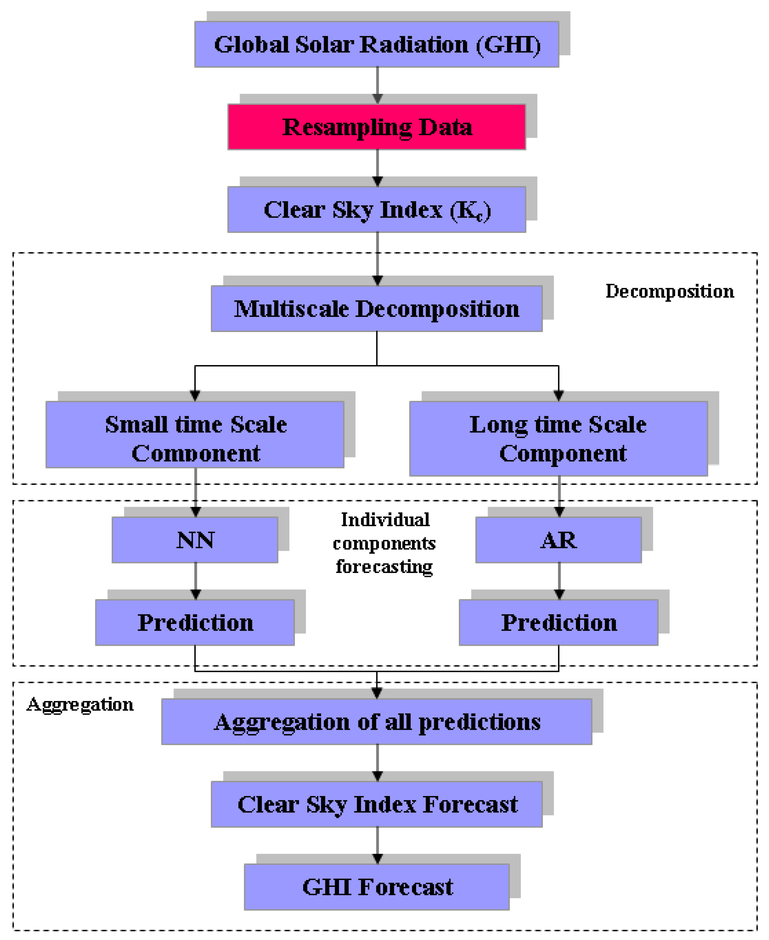
2.2. Forecast Model Method

The solar forecasting model proposed is described in [16]. The forecast modeling process is based on a hybrid AR model (linear forecasting process) and NN model (nonlinear forecasting process) combined with a multiscale decomposition method (Wavelet Decomposition, EMD (Empirical Mode Decomposition) and EEMD (Ensemble Empirical Mode Decomposition)). This model is a multiscale hybrid forecast model (MHFM). This hybrid model is built from a defined structure according to the flowchart in [16]. Its process is divided in several steps:
  • Step 1: Detrend the data estimating the clear sky index.
  • Step 2: Decompose the K c signal using a multiscale decomposition method (Empirical Mode Decomposition, Ensemble Empirical Mode Decomposition or Wavelet Decomposition). The choice of forecasting method is adaptive to the characteristic of each component.
  • Step 3: Forecast each multiscale decomposition component. The short time scales components are forecasted by NN model (non linear process) and the long time scales components are forecasted by the AR model (linear process).
  • Step 4: Sum all the component forecasts to obtain the final predicted time series.
  • Step 5: Rebuild the Global solar radiation signal from the predicted K c by using the Kasten Clear sky model.

2.3. Validation Metrics

The Hybrid forecast model performance can be evaluated using the following classical statistical performance indicators: relative MBE (rMBE) (Equation (3)), relative MAE (rMAE) (Equation (4)), relative RMSE (rRMSE) (Equation (5)), and skills scores (Equation (6)). These metric errors are typically used to evaluate the predictive performance of a solar forecast model. Relative error metrics are normalized to the mean observed irradiance data for the considered period [21], i.e., here, one year:
  • Relative Mean Biais Error ( r M B E )
    r M B E = 1 N i = 1 N ( p ^ i o i ) 1 N i = 1 N o i
  • Relative Mean Absolute Error ( r M A E )
    r M A E = 1 N i = 1 N | p ^ i o i | 1 N i = 1 N o i
  • Relative Root Mean Square Error ( r R M S E )
    r R M S E = 1 N i = 1 N ( p ^ i o i ) 2 1 N i = 1 N o i
    where o i is the observed value of GHI, p ^ i is the forecast value of GHI and N the number of point in the dataset for the considered period.
  • Skill s: Compare the model performance with a reference model [39]. In this study, the proposed model was compared with the persistence model applying the skill parameter proposed by Coimbra et al. [40]:
    s = ( 1 R M S E m o d e l R M S E S C p e r s ) × 100
    where index S C p e r s refers to the scaled persistence reference model defined by Equation (7).
    K c ^ ( t + h ) = K c ( t )
    The corresponding GHI forecast was obtained using Equation (8):
    G H I ^ ( t + h ) = G H I ( t ) × G H I c l e a r ( t + h ) / G H I c l e a r ( t )

2.4. Methods of MHFM Predictive Performance Analysis according to Forecast Horizons Parameters and Insolation Conditions Parameters

This section describes the methods and process which were used to analyze the influence of forecast horizon with two strategies on the predictive performance of MHFM and the influence of global solar radiation typical days on forecasting models errors.

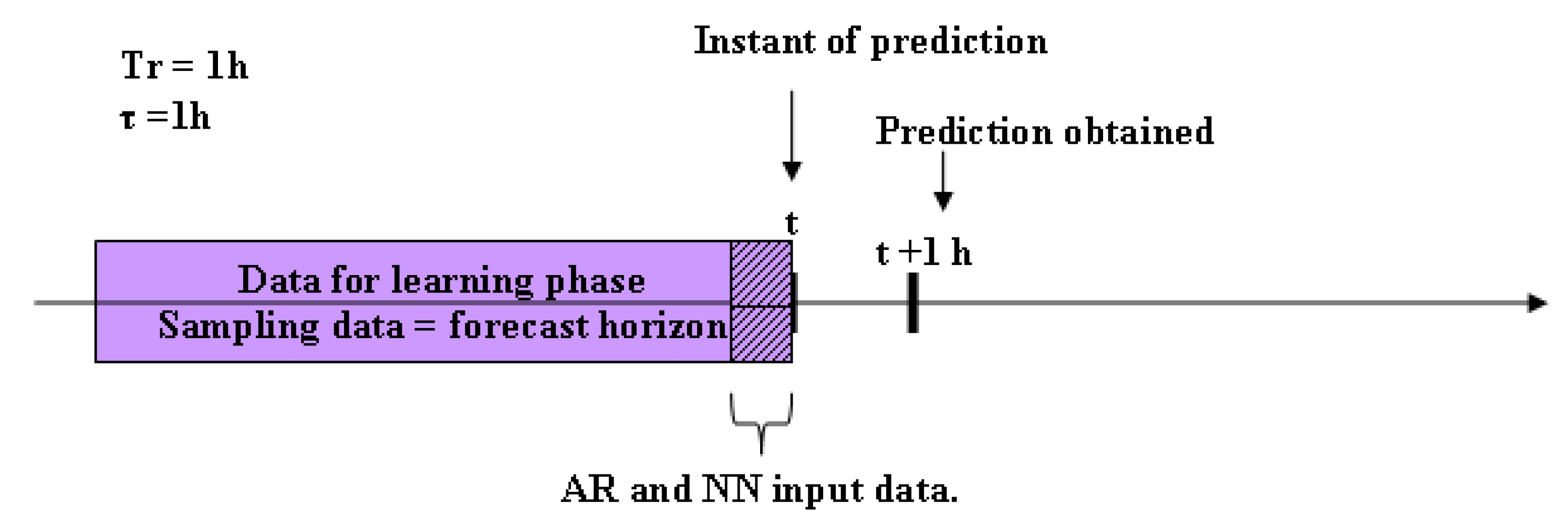
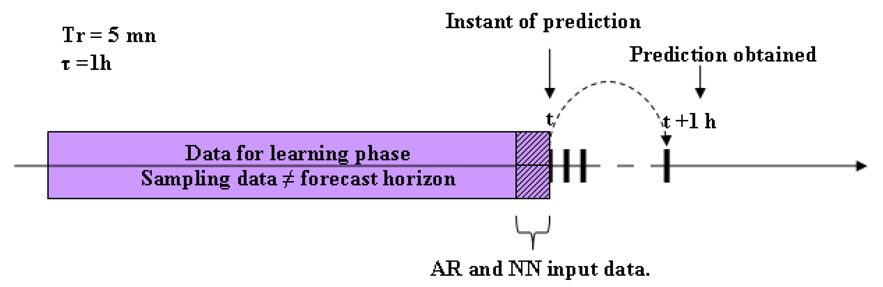
2.4.1. Methods of Forecast Horizon Modeling Process

According to categorization given in [41], our study focused on intra-hour and intra-day forecast horizons i.e., from 5 min to 6 h.
Strategy 1: Sampling data T r = forecast horizon τ The first strategy consists in resampling the input data such that the time sampling T r is equal to the time horizon τ . In this case, the model predicts directly the next point. Figure 2 briefly illustrates the individual components forecasting process for example, T r = τ = 1 h.
Strategy 2: sampling data T r ≠ forecast horizon τ In the second strategy, the time sampling is different to the time horizon ( T r τ ). The goal here is to verify if having higher frequency sampling learning data influences the MHFM performance. Intuitively, we could think that the more statistical information there is in the learning data, due to higher frequency sampling, the better is the forecasting performance. The second strategy consists in verifying this assumption. There is no additional step for input data compared to the first strategy; the learning data sampling T r = 5 min is the same for all the considered forecast horizon τ . Figure 3 briefly represents an example of the individual components forecasting phase for a τ = 1 h. This strategy is operated as follows for each decomposition components:
  • The number of input data is determined by the AIC and BIC criterion for the AR model and by the mutual information for the NN model [16,21] using a six-month dataset with sampling time T r = 5 min. The number of input found would be valid for all considered forecast horizons τ .
  • To provide a forecasting at t + τ with a six-month data test, the data test sampling time is also 5 min and the model allows us to obtain every 5 min the forecast at t + τ .
In summary, this approach performs the AR and NN learning phase with 5 min data sampling and provides a forecasting at t + τ , with the time horizon 5 τ 360 min (6 h).

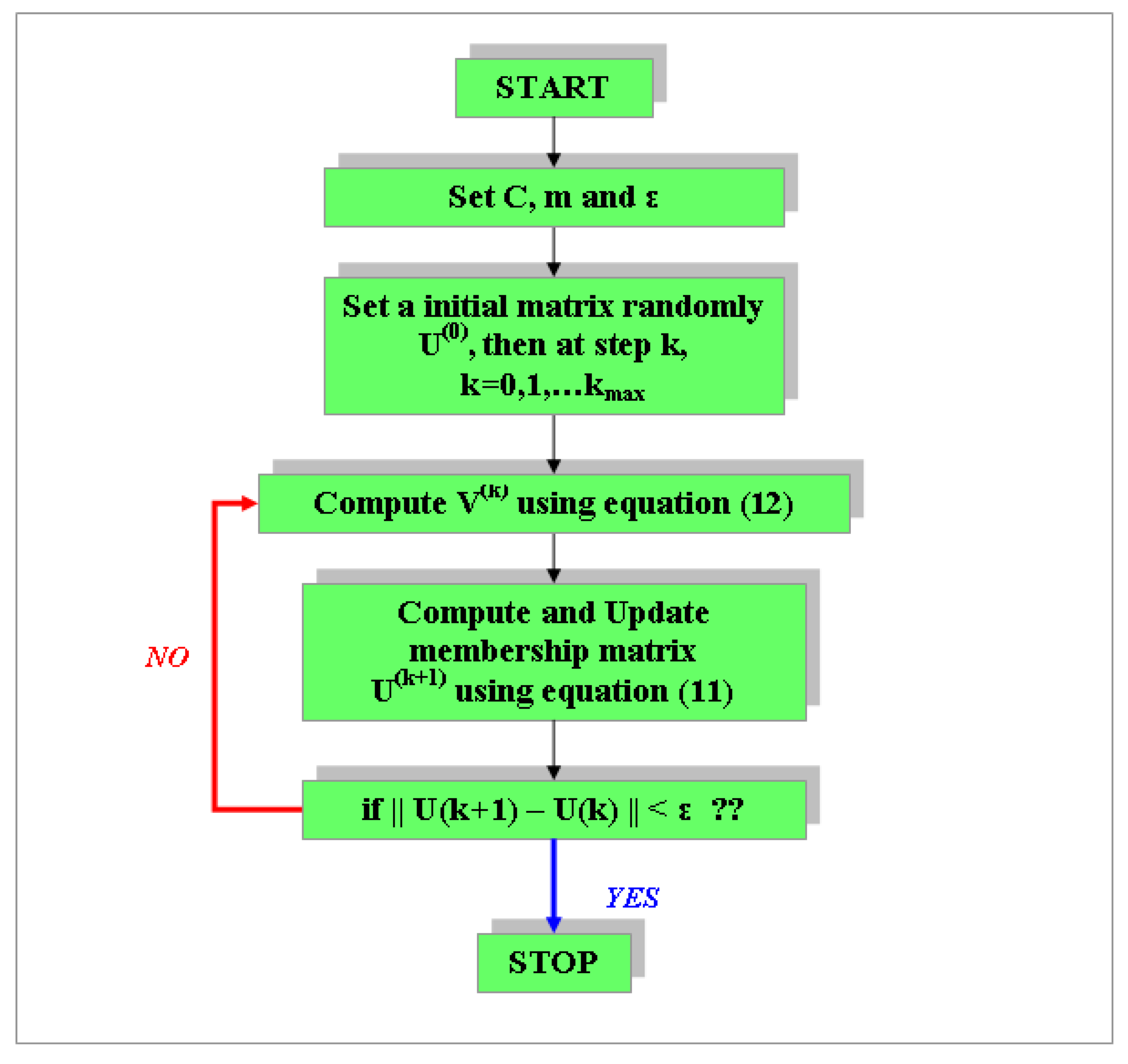
2.4.2. Method of Insolation Conditions Classification

To illustrate the performance of MHFM model as a function of insolation conditions, days were categorized as a function of their variability. A classification of daily irradiance profiles was performed. Often, in the literature, in solar area, the k-means method is used [13,27,36]. Recently, the Fuzzy C-means clustering is used for the implementation of demand side management measures [42] or to classify global horizontal irradiance [28]. This clustering technique is an iterative method to classify individuals (or samples) in C classes. It was introduced by Ruspini [43], and later extended by Dunn and Bezdek [44,45]. It determines the centers of the classes and generates the matrix to estimate the membership of individuals, to one of the predefined classes. The main purpose of this method is to minimize a cost function, which is usually chosen to be the total distance between each sample to the center of each class [45,46].
J ( U , V ) = k = 0 n i = 1 C μ i k m x i k v i
n is the total number of samples, C is the predefined number of classes, x k is the vector representing the kth individual, v i is the vector representing the center of the ith class and μ i k is the degree of membership of the kth individual in the ith class. The matrix U contains the coefficients μ i k . V is the matrix containing the center of the C classes v i and m is a constant greater than 1 (generally m = 2 ). By differentiating the function J ( U , V ) according to v i , keeping U constant and according to μ i k , keeping V constant, the following equations are obtained [45]:
μ i k = 1 j = 1 C ( x k v i x k v j ) 2 ( m 1 )
V i = j = 1 n ( μ i k ) m x k j = 1 n ( μ i k ) m
In Equations (9) and (10), the symbol . represents the Euclidian distance.
Figure 4 presents the flowchart of Fuzzy-C-means algorithm.

Validity Criterion

We used a validity criterion to determine the optimal numbers of classes and “fuzzy factor value”. It is defined by a fuzzy clustering validity function noted S, which measures the overall average and the separation of a fuzzy-C partition [47]. S can be explicitly written as:
S = i = 1 C j = 1 n μ i j m V i X j 2 n × ( d m i n ) 2
where d m i n represents the minimum euclidian distance between cluster centroids, i.e.,
d m i n = m i n i , j V i V j
The class number (or “fuzzy factor value”) is optimal for the smallest value of S.

3. Results

In this section, firstly the results of our analysis on the MHFM predictive performance are presented as a function of the two forecast horizon strategies previously described in this paper (Section 2.4.1). The second part of the results concern illustrating the MHFM performance as a function of daily insolation conditions shown by a study of forecasting error metrics based on typical days obtained by the classification using Fuzzy-C means method.

3.1. Influence of the Forecast Horizons Strategy on Performance Model

In this study, time horizons of 5, 10, 15, 30 min, 1 h, 2 h, 4 h and 6 h, were tested.

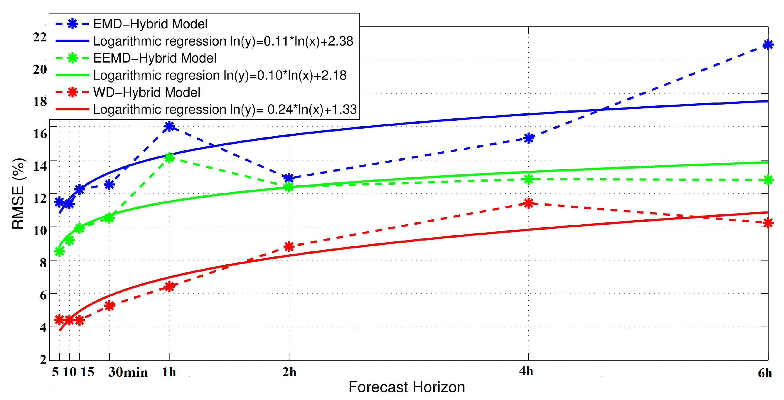
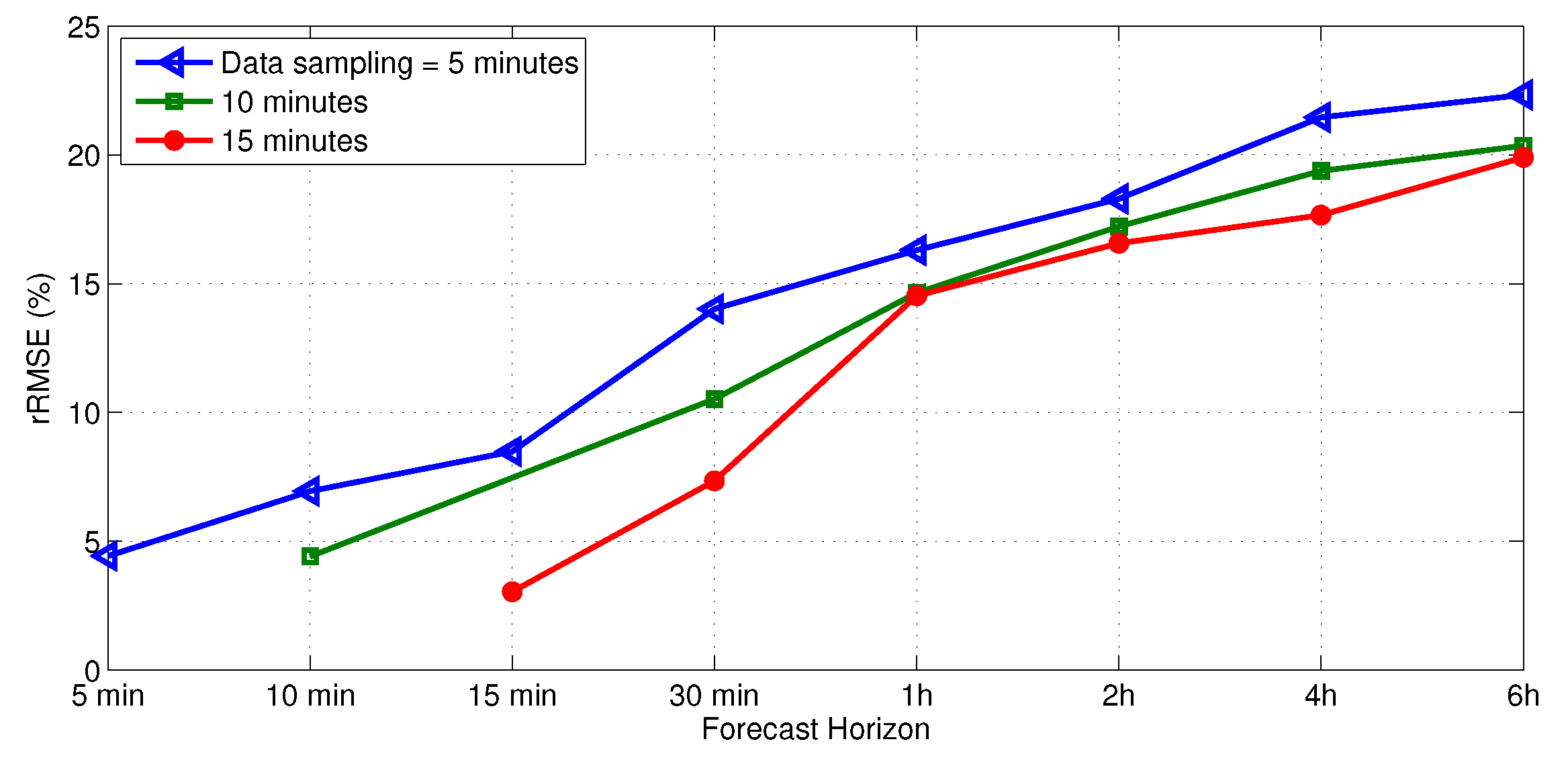
3.1.1. Results: Strategy 1: Sampling Data = Forecast Horizon

Note that, in Strategy 1, the sampling time is equal to the forecast horizon. For example, for a horizon of 5 min, input data or learning dataset are sampled at 5 min and, for a horizon of 2 h, input data are sampled at 2 h. The initial dataset is sampled at 1 s. In the EMD case, the number N of intrinsic mode functions (IMF) is proportional to the length of the dataset [18]:
N = T n Δ t
where T represents the total data length, Δ t represents the digitizing rate and n represents the minimum number of Δ t needed to define the frequency accurately. Consequently, the longer is the horizon time. the smaller is the number of decomposition components.
Figure 5 illustrates the MHFM flowchart including the resampling step before the multiscale decomposition step.
Table 1 shows the Hybrid model forecasting performances using the first strategy. It can be noted that, whatever the multiscale decomposition-hybrid model chosen, the rRMSE error increased with the forecast horizon, as illustrated in Figure 6. This increase was nonlinear and seemed follow a logarithmic tendency. In agreement with Monjoly et al. [16], we found that the best results were obtained by the WD-Hybrid model (rRMSE varied between 4.41% and 11.42%). The skill parameters, which allow comparing the hybrid model performances to the persistence model, varied between 78.58% and 85.54%, highlighting a clear better performance of the proposed model compared to the persistence model, for all forecast horizons.

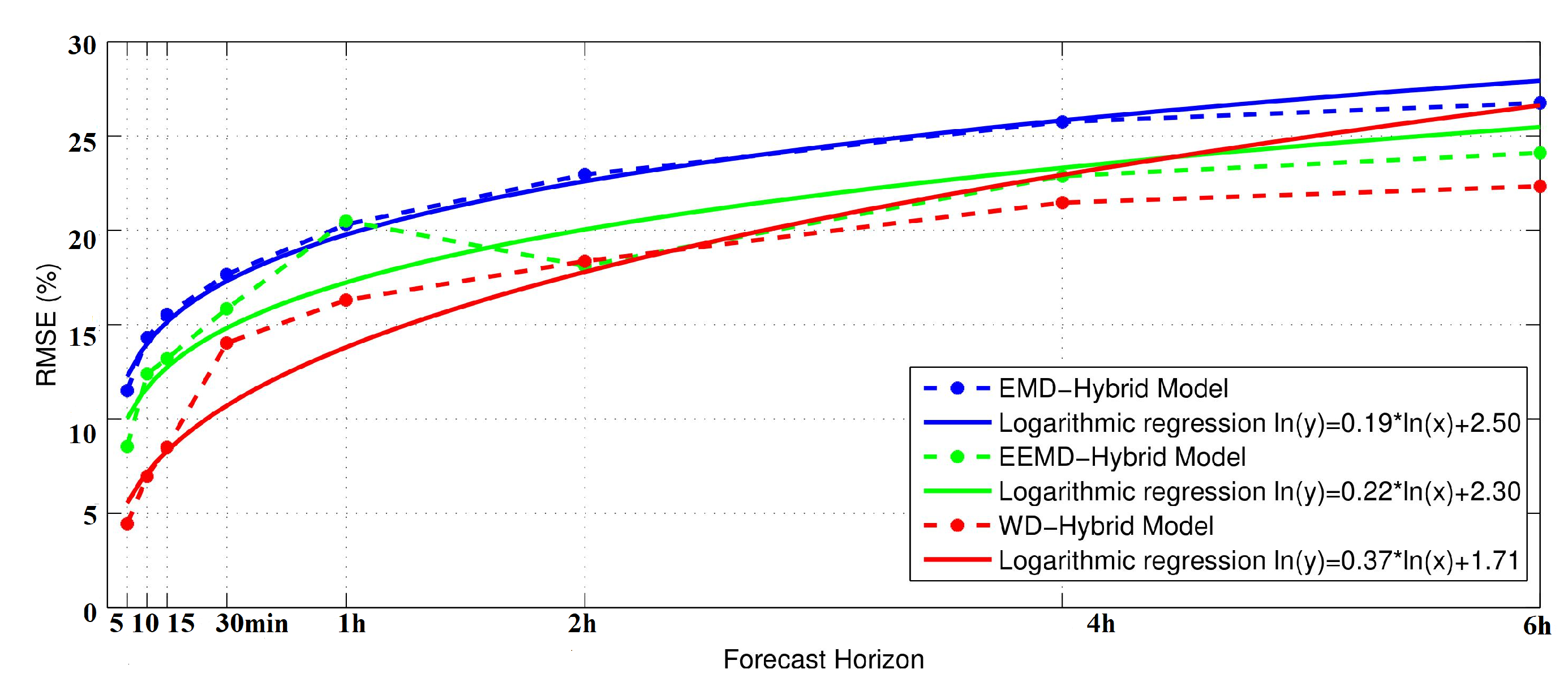
3.1.2. Results: Strategy 2: Sampling Data T r ≠ Forecast Horizon τ

The objective of the second strategy was to assess how the model’s performance evolves by using learning data with high frequency sampling ( T r = 5 min for all horizons). This approach uses 5 min data sampling to forecast the GHI at several horizons τ (from 5 min to 6 h). The AR and NN model learning phase is performed with 5 min data sampling and the forecast is directly obtained every 5 min at t + τ .
Figure 7 illustrates the MHFM flowchart with the second strategy. Table 2 draws up the forecasting performance of the Hybrid model according to the forecasting with a data sampling equals to 5 min.
With this approach, the WD-Hybrid Model presented the best results (rRMSE from 4.43 % to 22.33 % and skill parameter varied from 78.58 % to 7.81 % ). Figure 8 represents the rRMSE versus the forecast horizon compared to the associated logarithmic regression. We made the assumption that enriching the learning dataset by a higher frequency sampling would improve the model performance but the WD-hybrid model errors obtained by using the second strategy were higher than those obtained by the first strategy. Finally, to more accurately verify if the time scales of learning data influences the predictive performance of hybrid model with Strategy 2, the modeling process was performed with sampling learning data varying from 5 to 15 min. Figure 9 represents the rRMSE versus the forecast horizon for different learning data sampling and shows that the learning dataset time scale had an influence on the hybrid model performance. Nevertheless the results suggest that the first strategy was more efficient due to the effect of the sample on the model robustness.
Next, the influence of another parameter on the MHFM performance was investigated. In tropical zone, the irradiance time series present a high temporal variability. It is interesting to assess the influence of this phenomenon on the predictive performance of MHFM model. Consequently, the strengths and limitations of the proposed models were analyzed as a function insolation of conditions performed by a classification of typical days.

3.2. Solar Variability Influence on MHFM Performance

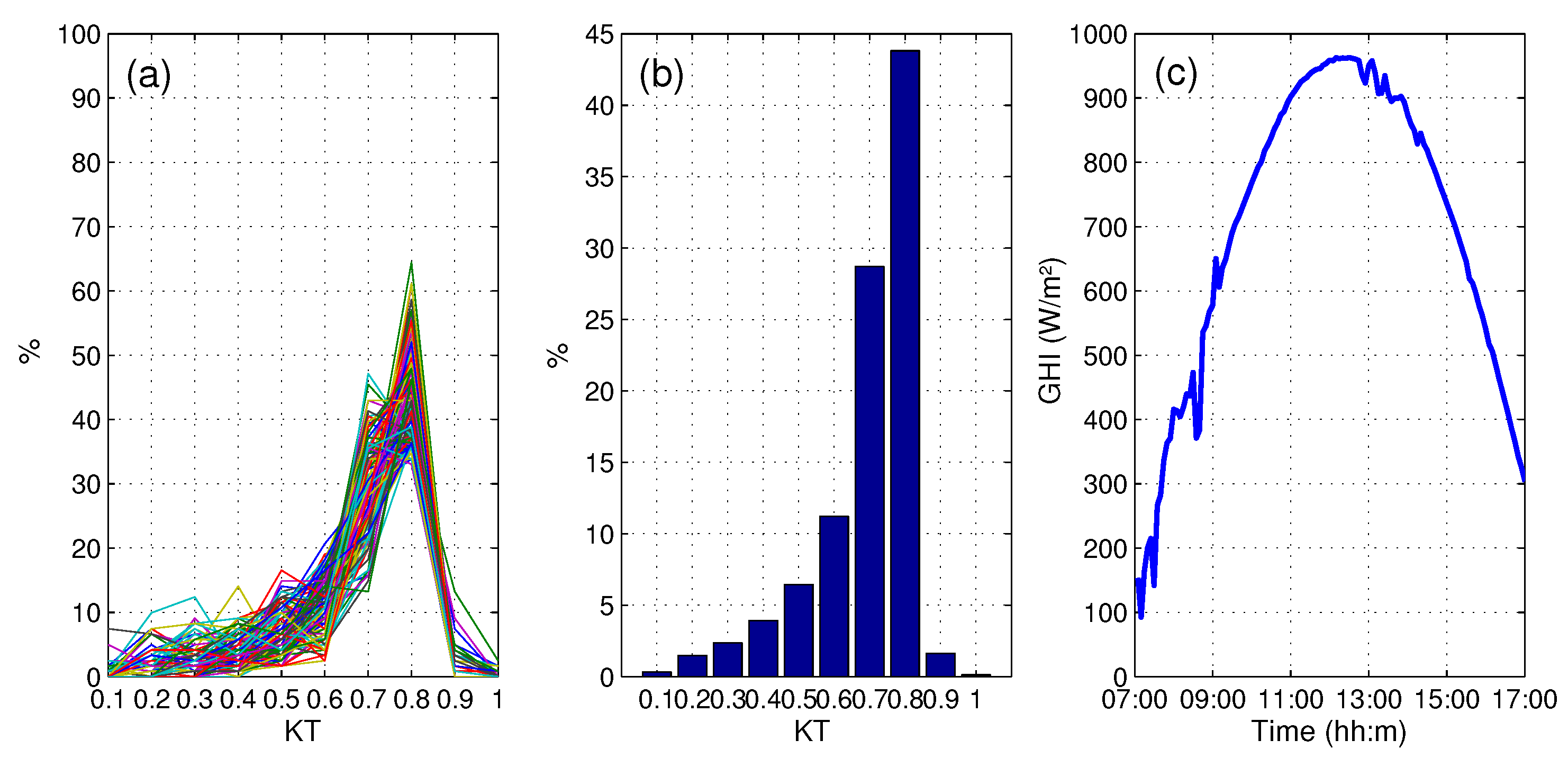
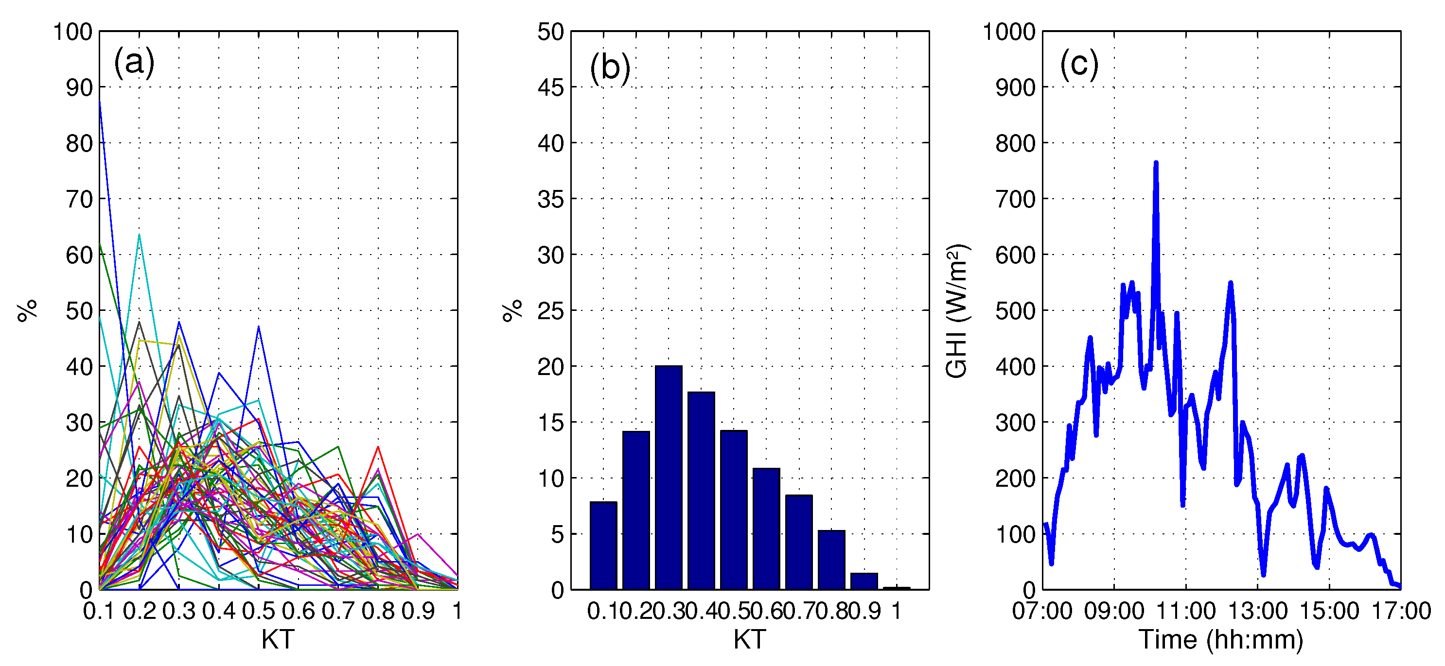
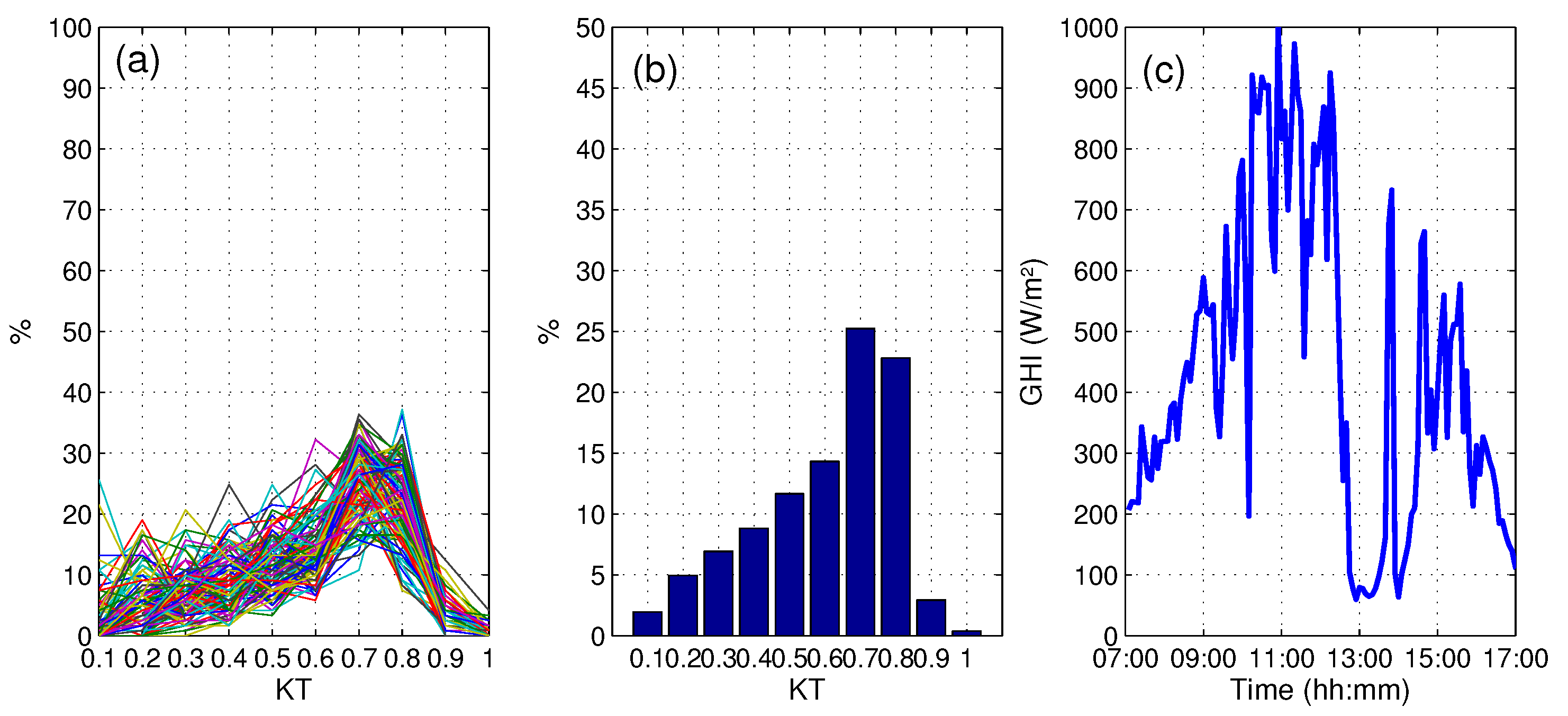
3.2.1. Results of Daily Irradiance Classification

In this study, the classification method, fuzzy c-means clustering, was applied to 366 days of Global solar radiation sampled at 5 min. The clearness index K t defined in Equation (2) was computed for each day to estimate the K t histograms.For this classification process, the fuzzy c-means cluster was applied on daily K t histograms. The fuzzy C means clustering algorithm was tested for several numbers of classes C = 2 , 3 , 4 , 5 , 6 . The validation criterion, given in Equation (12), allowed defining that the optimum number of classes was 4: the S value corresponding to each number of cluster is drawn up in Table 3. In Soubdhan et al. [25], a classification of K t in using k-means method shows four classes of typical days. The results uncovered four classes corresponding to four types of days: clear sky day, intermittent clear sky day, intermittent cloudy day and cloudy day. Our results are in agreement with those obtained by Soubdhan et al. in [25].
  • Clear sky day (CS)
    In 2012, clear sky day events represented 29 % of GHI days of the year (Table 4). This type of days has very few cloudy passages (Figure 10c). The clear sky day K t distribution has a maximum of occurrence value ( 44 % ) around K t = 0.8 (Figure 10a). Figure 10b shows that around 86 % of K t values [ 0.5 ; 1 ] .
  • Intermittent clear sky day (ICS)
    This second class represents 24 % of events (Table 4). This type of days has an important solar radiation but the cloudy passages are frequent (Figure 11c). The K t distribution has a maximum occurrence value ( 47 % ) around K t = 0.7 and around 80 % of K t values [ 0.5 ; 1 ] (Figure 11b).
  • Cloudy Sky day(ClS)
    The cloudy sky day has important slow cloudy passages (Figure 12c). This class is the least represented representing 17 % of the days in 2012 (Table 4). The K t distribution has a maximum occurrence ( 20 % ) around K t = 0.3 and around 73% of K t values [ 0 ; 0.5 ] (Figure 12b).
  • Intermittent cloudy sky day(IClS)
    For an intermittent cloudy sky day, important cloudy passages are observed (Figure 13c). This class represented 111 days in 2012 or 30 % of the year (Table 4). The K t distribution haa a maximum occurrence ( 25 % ) around K t = 0.7 and around 63 % of K t values [ 0.5 ; 1 ] (Figure 13b).
In the following experiment, the characterization of the variability of each typical days previously mentioned was investigated. For this investigation, a statistical parameter that highlights the ramp rate magnitude was used.

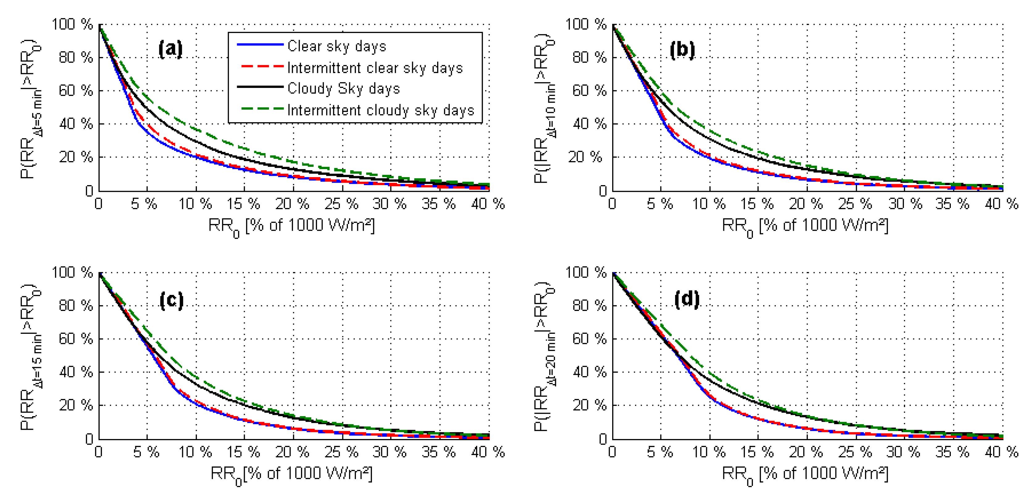
3.2.2. Variability Characterization of Each Day Class

To categorize typical days as a function of their variability, the amplitude of fluctuations for different time scales was studied. In Lave et al. [31], the dynamic of irradiation day is characterized by the variability score. The variability score is defined as the maximum value of ramp rate magnitude ( R R 0 ) times ramp rate probability (Equation (15)). The variability score was determined using the cumulative distribution function of ramp rates using a given timescale [32].
V S ( Δ t ) = 100 × max ( R R 0 . P ( | R R Δ t | > R R 0 ) )
where Δ t represents the time scale, and R R 0 and R R Δ t are a percent of Standard Test Conditions (STC) irradiance = 1000 W·m 2 . The probability P ( | R R Δ t | > R R 0 ) represents the fraction of time where the absolute value of R R Δ t is higher than R R 0 . As in [31], we chose to use the moving averages definition of ramp rates R R Δ t given by Kleissl [48]:
R R Δ t ( t ) = 1 Δ t ( t t + Δ t G H I t Δ t t G H I )
Figure 14 presents the Δ t -cumulative distribution of GHI ramp rate for each class and for different time scales. At Δ t = 5 min, in Figure 14a, 65% of ramp rates for the clear sky days are lower than 50 W·m 2 concerning clear sky days. This probability reaches 60 % for the intermittent clear sky days, 50 % for the cloudy sky days and 45 % for the intermittent cloudy sky days. Compared with the intermittent cloudy sky days, the cloudy days present a lower occurrence of having ramp rate of low amplitude (<50 W·m 2 ). We can note that the more the time scales increase, the more the occurrence of having ramp rates higher than 50 W·m 2 increases (Figure 14b–d). Moreover, the probability of ramp rate is quasi equal to those of clear sky days and intermittent clear sky days for this range. For Δ t = 15 and 20 min, when R R 0 reaches 25% of STC (250 W·m 2 ), the cloudy sky day and intermittent cloudy sky days cumulative distribution (respectively, clear sky days and intermittent clear sky days cumulative distribution) eventually have the same behavior. This study supports the characterization of the different typical days class. Indeed, the results reveal a higher magnitude of ramps rate and higher occurrence of these ramps for intermittent cloudy days and cloudy days, therefore more extreme events of insolation conditions for these typical days. This observation is all the more relevant as the time scales of Δ t increase.
The Variability Score (VS) over timescale Δ t (Figure 15) is presented. For each class, VS is shown to increase over Δ t . For all considered time scales, the intermittent cloudy sky days is the most variable and the clear sky day the less variable. In [31], Lave et al. made the same observation. They determined the VS over Δ t for 10 sites in USA considering Δ t = 1 s, 10 s, 30 s, 60 s and 3600 s and demonstrated that VS increases over Δ t .
Variability samples with high V S values (intermittent cloudy days or cloudy days) can be expected to have a large impact on predictive performance, while variability samples with low V S values aree expected to have less of an impact. In the next section, the results of MHFM predictive performance are exposed according to the type of days.

3.2.3. Variability Influence on Hybrid Forecast Model Performances

Six months of data were used for the training stage and the six following months for test data (forecasting stage). The forecast errors were calculated daily, then the days of the same class were grouped and an average of the errors was obtained. The results according to each class and each hybrid models are summarized in Table 5 for a forecast horizon of 5 min. It is noted that the best performance was obtained with the WD-Hybrid model. The clear sky days showed the lowest error metrics ( r R M S E = 2.91 % ) . On most days, forecasts matched observations almost perfectly due to their low daily variability demonstrated in Section 3.2.1. As previously mentioned in Section 3.2.1, the most variable days are the intermittent cloudy sky days. However, the MHFM predictive performance for this type of days ( r R M S E = 5.48 % ) was better than that obtained for cloudy sky days ( r R M S E = 6.73 % ) . Consequently, the variability of GHI signal is not the only factor able to influence the forecast error. The cloudy sky days are indeed the second most variable type of day but also representative of completely cloudy sky days with big size clouds having a slow speed. In this case, the solar radiation is mainly scattered by clouds and the daily profile irradiance is very low (very low GHI, usually < 600 W·m 2 ). Moreover, the cloudy sky day r M B E obtained with the WD-Hybrid Model was the highest ( r M B E = 0.32 % ) . The three others type of day being the most frequent (Table 4) during the training NN and AR stage, the hybrid model rarely met the cloudy sky days’ GHI signal and finally overestimated their forecasts. All these observations show that the combination of high variability (high ramp rate) and low daily GHI profile are the source of a lower predictive performance of the model for cloudy sky days class. Nevertheless, the robustness of MHFM allows limiting their effects on the quality of the forecast to obtain a rRMSE lower than 7 % .

4. Discussion

The very small size of islands, their complex topography (mountainous orography and land/sea contrasts) and frequent cloud formation lead to a diversity of solar microclimates. This environment induces high spatial and temporal variability, particularly at short time scales [21,36,49]. Consequently, solar radiation forecasting is challenging. Thus, the strengths and limitations of MHFM model were assessed when used on a location with this challenging environment. For this, in this study, the performance of several forecasting approaches of MHFM were assessed for different time horizon and strategies of process time horizon but also based on daily insolation conditions. Several studies showed the evolution of predictive performance forecast techniques based on time horizon. In [50], spatiotemporal kriging is tested for short time horizons (from 30 s to 300 s) using the same time resolution and time horizon (Strategy 1 in this paper). For forecast techniques such as persistence, ARIMA, NN, SVM, and ML algorithms, they are tested for various time horizon different from time resolution of input data (Strategy 2) (e.g., [22,24,51,52]). In the literature, for the first time, the same forecast techniques were tested for various forecast horizons with different process strategies for the time horizon. Two strategies for the forecast at several horizons are proposed: the first method is to have the same time scale of temporal resolution and time forecast horizon; the second is to have a shorter time scale (5 min, 10 min, or 15 min) for learning data than time forecast horizon (from 5 min to 6 h). As in [16], the hybrid model was tested for threemultiscale decomposition methods (EMD, EEMD and WD). With the first and the second strategy, whatever the multiscale decomposition-hybrid model chosen the rRMSE values increase with the time forecast horizon. Moreover, the results highlighted the fact that smaller time scales of learning data than time scales of data test, did not improve the accuracy of forecasts. For example, if we want an accurate forecasting at 30 min time horizons, it is not relevant to use 5 min or 15 min time scale learning data. This means that the increasing of statistical information by smaller time scale does not improve, and may complicate the learning phase to forecast at a higher time scale. It is also noted, as demonstrated by Monjoly et al. in [16], that the best results were obtained with the WD-Hybrid model (first strategy: rRMSE varying between 4.41% and 11.42%; second strategy: rRMSE varying from 4.43 % to 22.33 % ). Moreover, we analyzed the influence of the global solar variability upon the forecasting error of different multiscale decomposition models. Two comments can be given. We then established a dataset of four classes of typical days in accordance with previous studies from literature: clear sky day, intermittent clear sky day, cloudy sky and intermittent cloudy sky. We used other statistical parameters to characterize the variability of each class such as the variability score and magnitude of ramp rate. Firstly, the results reveal that the variability of insolation conditions was not the only factor that decreased forecast accuracy. Indeed, the daily profile of irradiance was an influence factor. These analysis were supported by the study of cumulative distribution of ramp rates and VS scores. In other works, we may develop a parameter which may give accurate information on daily irradiance profile. Secondly, the results are particularly relevant for WD- hybrid model. All these statistical analyses characterize and highlight different parameters influencing the accuracy of our forecast models and, certainly, can be used as a reference and applied to other forecast techniques in the literature to evaluate their limits. These analyses can be used by other models to evaluate the robustness of their modeling process: (1) analysis to verify if shorter time scales in data, i.e., a more complex use of the information contained in the time series of learning data, are more appropriate or not to the model; (2) analysis verifying the daily insolation conditions and their influence on the predictive performance of the model; and (3) analysis of the daily variability reinforced by the study of cumulative distribution of ramp rates and VS scores. These steps can be used for a benchmarking of several techniques of models. Moreover, the obtained results highlighting a relevant predictive performance for WD-hybrid model show in terms of decisional factors that, operationally, such an approach would mesh seamlessly with operational industry-targeted forecast services that exploit ground solar data resources.

5. Conclusions

The main cause of variability in surface solar irradiance is the motion/evolution of clouds. This is a particularly acute issue when considering grid-connected PV development for small island grids that are not interconnected without a possibility of spatial smoothing. Moreover, solar radiation forecasting is challenging because of lot of microclimates and high temporal variability. Consequently, a performant forecast model is needed. In [16], we proposed hybrid forecast models combining AR and NN models with the integration of multiscale decomposition methods (MD). This new model MHFM was successfully applied for solar radiation forecasting demonstrating a good predictive performance for 1 h ahead. To assess the robustness of this model, we tested the influence of various parameters on the accuracy of irradiance forecasting. The influence of time sampling combined with the forecast horizon and the influence of irradiance variability on the hybrid forecast model performances are the parameters that were tested. The results of this study suggest that the forecast horizon strategy based on the resampling of learning data (first strategy) is the most efficient. In this study, we also analyzed the influence of the global solar variability upon the forecasting error of different models. To categorize days as a function of their variability, a classification of typical days was performed, using a fuzzy c-means cluster on daily clearness index time series. As expected, the intermittent cloudy sky days was the most variable and the clear sky day the least variable. However, the predictive performance of models as a function of each class of typical day showed that the worst results were not obtained with the most variable class (intermittent cloudy sky). This study highlighted that the variability of GHI signal is not the only parameter able to influence the forecasting: the low daily GHI profile is another one (profile of cloudy days). This reveals the weakness of the hybrid model for these cases qualified as extreme events. Consequently, in future works, the hybrid model should be improved in this way. One remaining aspect to reflect upon consists in developing a parameter identifying the profile of daily irradiance. This parameter should strengthen our hypothesis and in future works could be integrated in the modeling process. The different proposed parameters can be useful tools for quantifying the predictive performance and the influence of irradiance forecasting accuracy. These analyses can strengthen the study of the performance of other techniques in the literature.

Author Contributions

S.M. contributed to analyses; M.A. contributed to writing the manuscript; R.C. contributed to the supervision and the general design of the manuscript; and T.S. contributed to the review and editing of the manuscript.

Funding

This research received no external funding.

Conflicts of Interest

The authors declare no conflict of interest.

References

  1. Yang, D.; Kleissl, J.; Gueymard, C.A.; Pedro, H.T.; Coimbra, C.F. History and trends in solar irradiance and PV power forecasting: A preliminary assessment and review using text mining. Solar Energy 2018, 168, 60–101. [Google Scholar] [CrossRef]
  2. Zhu, H.; Li, X.; Sun, Q.; Nie, L.; Yao, J.; Zhao, G. A power prediction method for photovoltaic power plan based on wavelet decomposition and artificial neural networks. Energies 2016, 9, 11. [Google Scholar] [CrossRef]
  3. Ogliari, E.; Grimaccia, F.; Leva, S.; Musetta, M. Hybrid Predictive Models for Accurate Forecasting in PV Systems. Energies 2013, 6, 1918–1929. [Google Scholar] [CrossRef] [Green Version]
  4. Khatib, T.; Mohamed, A.; Sopian, K. A review of solar energy modeling techniques. Renew. Sustain. Energy Rev. 2012, 16, 2864–2869. [Google Scholar] [CrossRef]
  5. Ahmed, O.; Driss, Z.; Hanane, D.; Rachid, B. Artificial neural network analysis of Moroccan solar potential. Renew. Sustain. Energy Rev. 2012, 16, 4876–4889. [Google Scholar]
  6. Mellit, A.; Kalogirou, S.; Hontoria, L.; Shaari, S. Artificial intelligence techniques for sizing photovoltaic systems: a review. Renew. Sustain. Energy Rev. 2009, 13, 406–419. [Google Scholar] [CrossRef]
  7. Sharma, V.; Yang, D.; Walsh, W.; Reindl, T. Short term solar irradiance forecasting using a mixed wavelet neural network. Renew. Energy 2016, 90, 481–492. [Google Scholar] [CrossRef]
  8. Gutierrez-Corea, F.V.; Manso-Callejo, M.A.; Moreno-Regidor, M.P.; Manrique-Sancho, M.T. Forecasting short-term solar irradiance based on artificial neural networks and data from neighboring meteorological stations. Solar Energy 2016, 134, 119–131. [Google Scholar] [CrossRef]
  9. Kashyap, Y.; Bansal, A.; Sao, A.K. Solar radiation forecasting with multiple parameters neural networks. Renew. Sustain. Energy Rev. 2015, 49, 825–835. [Google Scholar] [CrossRef]
  10. Huang, J.; Korolkiewicz, M.; Agrawal, M.; Bol, J. Forecasting solar radiation on an hourly time scale using a Coupled AutoRegressive and Dynamical System (CARDS) model. Solar Energy 2013, 87, 136–149. [Google Scholar] [CrossRef]
  11. Sun, H.; Yan, D.; Zhao, N.; Zhou, J. Empirical investigation on modeling solar radiation series with ARMA–GARCH models. Energy Convers. Manag. 2015, 92, 385–395. [Google Scholar] [CrossRef]
  12. André, M.; Dabo-Niang, S.; Soubdhan, T.; Ould-Baba, H. Predictive spatio-temporal model for spatially sparse global solar radiation data. Energy 2016, 111, 599–608. [Google Scholar] [CrossRef]
  13. André, M.; Perez, R.; Soubdhan, T.; Schlemmer, J.; Calif, R.; Monjoly, S. Preliminary assessment of two spatio-temporal forecasting technics for hourly satellite-derived irradiance in a complex meteorological context. Solar Energy 2019, 177, 703–712. [Google Scholar] [CrossRef]
  14. Reikard, G.; Hansen, C. Forecasting solar irradiance at short horizons: Frequency and time domain models. Renew. Energy 2019, 135, 1270–1290. [Google Scholar] [CrossRef]
  15. Zhang, G. Time series forecasting using a hybrid ARIMA and neural network model. Neurocomputing 2003, 50, 159–175. [Google Scholar] [CrossRef]
  16. Monjoly, S.; André, M.; Calif, R.; Soubdhan, T. Hourly forecasting Global Solar radiation based on Multiscale decomposition methods—A hybrid Approach. Energy 2017, 119, 288–298. [Google Scholar] [CrossRef]
  17. Daubechies, I. The wavelet transform time-frequency localization and signal analysis. IEEE Trans. Inform. Theory 1990, 36, 961–1004. [Google Scholar] [CrossRef]
  18. Huang, N.E.; Shen, Z.; Long, S.R.; Wu, M.C.; Shih, H.H.; Zheng, Q.; Yen, N.C.; Tung, C.C.; Liu, H.H. The empirical mode decomposition and the Hilbert sprectrum for nonlinear and non-stationnary time series analysis. Proc. R. Soc. Lond. 1998, 454, 903–995. [Google Scholar] [CrossRef]
  19. Lei, Y.; He, Z.; Zi, Y. Application of the EEMD method to rotor fault diagnosis of rotating machinery. Mech. Syst. Signal Process 2009, 23, 1327–1338. [Google Scholar] [CrossRef]
  20. Reikard, G. Predicting solar radiation at high resolutions: A comparison of time series forecasts. Solar Energy 2009, 83, 342–349. [Google Scholar] [CrossRef]
  21. Lauret, P.; Voyant, C.; Soubdhan, T.; Mathieu, D.; Poggi, P. A benchmarking of machine learning technique for solar radiation forecasting in an insular context. Solar Energy 2015, 112, 446–457. [Google Scholar] [CrossRef]
  22. Dobbs, A.; Elgindy, T.; Hodge, B.M.; Florita, A. Short-Term Solar Forecasting Performance of Popular Machine Learning Algorithms. In Proceedings of the International Workshop on the Integration of Solar Power into Power Systems (Solar Integration Workshop), Berlin, Germany, 24–25 October 2017. [Google Scholar]
  23. Sakshi, M.; Praveen, P. Multi-time-horizon Solar Forecasting Using Recurrent Neural Network. In Proceedings of the 2018 IEEE Energy Conversion Congress and Exposition (ECCE), Portland, OR, USA, 23–27 September 2018; pp. 18–24. [Google Scholar] [CrossRef]
  24. Reikard, G.; Haupt, S.E.; Jensen, T. Forecasting ground-level irradiance over short horizons: Time series, meteorological, and time-varying parameter models. Renew. Energy 2017, 112, 474–485. [Google Scholar] [CrossRef]
  25. Soubdhan, T.; Emilion, R.; Calif, R. Classification of daily solar radiation distributions using a mixture of Dirichlet distributions. Solar Energy 2009, 83, 1056–1063. [Google Scholar] [CrossRef] [Green Version]
  26. Muselli, M.; Poggi, P.; Notton, G.; Louche, A. Classification of typical Meteorological Days from Global Irradiation Records ad Comparison Between Two Mediterranean Coastal Sites in Corsica Island. Energy Convers. Manag. 2000, 41, 1043–1063. [Google Scholar] [CrossRef]
  27. Soubdhan, T.; Abadi, M.; Emilion, R. Time Dependent Classification of Solar Radiation Sequences Using Best Information Criterion. Energy Procedia 2014, 57, 1309–1316. [Google Scholar] [CrossRef] [Green Version]
  28. Benmouiza, K.; Tadj, M.; Cheknane, A. Classification of Hourly Solar Radiation using Fuzzy-C means algorithm for optimal stand-alone PV system sizing. Electr. Power Energy Syst. 2016, 82, 233–241. [Google Scholar] [CrossRef]
  29. Johnson, J.; Schenkman, B.; Ellis, A.; Quiroz, J.; Lenox, C. Initial operating experience of the 1.2-MW La Ola photovoltaic system. In Proceedings of the 38th IEEE Photovoltaic Specialists Conference (PVSC), Austin, TX, USA, 3–8 June 2012; Volume 2, pp. 1–6. [Google Scholar]
  30. Hansen, C.; Stein, J.; Ellis, A. Statistical Criteria for Characterizing Irradiance Time Series; Sandia National Laboratories: Albuquerque, NM, USA, 2010.
  31. Lave, M.; Reno, M.J.; Broderick, R.J. Characterizing local High-frequency solar variability and its impact to distribution studies. Solar Energy 2015, 118, 327–337. [Google Scholar] [CrossRef]
  32. Gagné, A.; Turcotte, D.; Goswamy, N.; Poissant, Y. High resolution characterisation of solar variability for two sites in Eastern Canada. Solar Energy 2016, 137, 46–54. [Google Scholar] [CrossRef]
  33. Perez, R.; Kivalov, S.; Schlemmer, J.; Hemker, K.; Hoff, T.E. Short-term irradiance variability: Preliminary estimation of station pair correlation as a function of distance. Solar Energy 2012, 86, 2170–2176. [Google Scholar] [CrossRef]
  34. Dambreville, R.; Blanc, P.; Chanussot, J.; Boldo, D. Very short term forecasting of the global horizontal irradiance using a spatio-temporal autoregressive model. Renew. Energy 2014, 72, 291–300. [Google Scholar] [CrossRef]
  35. Kasten, F. A simple parametrization of two pyrheliometric formulae for detremining the linke turbidity factor. Meteorol. Rundsch. 1980, 33, 124–127. [Google Scholar]
  36. Badosa, J.; Haeffelin, M.; Chepfer, H. Scales of spatial and temporal variation of solar irradiance on Reunion tropical island. Solar Energy 2013, 88, 42–56. [Google Scholar] [CrossRef]
  37. Jiménez-Pérez, P.; Mora-López, L. Modelling and Forecasting hourly Global Solar Radiation using Clustering and Classification techniques. Solar Energy 2016, 135, 682–691. [Google Scholar] [CrossRef]
  38. Kasten, F. The link Turbidity Factor Based on Improved Values of integral Rayleigh Optical thickness. Solar Energy 1996, 56, 239–244. [Google Scholar] [CrossRef]
  39. Bacher, P.; Madsen, H.; Nielsen, H.A. Online short-term solar power forecasting. Solar Energy 2009, 83, 1772–1783. [Google Scholar] [CrossRef] [Green Version]
  40. Coimbra, C.F.M.; Kleissl, J.; Marquez, R. Overview of Solar Forecasting Method and a metric for accuracy evaluation. In Solar Energy Forecasting and Resource Assessment; Kleissl, J., Ed.; Elsevier: Amsterdam, The Netherlands, 2013; pp. 171–194. [Google Scholar]
  41. Diagne, M.; David, M.; Lauret, P.; Boland, J.; Schmutz, N. Review of Solar irradiance forecasting methods and a proposition for small scale insular grids. Renew. Sustain. Energy Rev. 2013, 27, 65–76. [Google Scholar] [CrossRef]
  42. Panapakidis, I.; Asimopoulos, N.; Dagoumas, A.; Christoforidis, G.C. An Improved Fuzzy C-Means Algorithm for the Implementation of Demand Side Management Measures. Energies 2017, 10, 1407. [Google Scholar] [CrossRef]
  43. Ruspini, E.H. Numerical Methods for fuzzy clustering. Inf. Sci. 1970, 2, 319–350. [Google Scholar] [CrossRef]
  44. Dunn, J.C. A fuzzy relative of ISODATA process and its use in clustering compact and well separated cluster. J. Cybern. 1974, 3, 32–57. [Google Scholar] [CrossRef]
  45. Bezdek, J.C. Pattern Recognition with Fuzzy Objective Function Algorithms; Kluwer Academic Publishers: Norwell, MA, USA, 1981. [Google Scholar]
  46. Bezdek, J.; Ehrlich, R. Numerical Methods for fuzzy clustering. Comput. Geosci. 1984, 10, 191–203. [Google Scholar] [CrossRef]
  47. Xie, X.; Beni, G. A validity measure for fuzzy clustering. IEEE Trans. Pattern Anal. Mach. Intell. 1991, 8, 841–847. [Google Scholar] [CrossRef]
  48. Kleissl, J. Solar Energy Forecasting and Resource Assessment; Academic Press: Cambridge, MA, USA, 2013. [Google Scholar]
  49. Cécé, R.; Bernard, D.; Brioude, J.; Zahibo, N. Microscale anthropogenic pollution modelling in a small tropical island during weak trade winds: Lagrangian particle dispersion simulations using real nested LES meteorological fields. Atmos. Environ. 2016, 139, 98–112. [Google Scholar] [CrossRef]
  50. Aryaputera, A.W.; Yang, D.; Zhao, L.; Walsh, W.M. Very short-term irradiance forecasting at unobserved locations using spatio-temporal kriging. Solar Energy 2015, 122, 1266–1278. [Google Scholar] [CrossRef]
  51. Tato, J.H.; Brito, M.C. Using Smart Persistence and Random Forests to Predict Photovoltaic Energy Production. Energies 2019, 12, 100. [Google Scholar] [CrossRef]
  52. Du, J.; Min, Q.; Zhang, P.; Guo, J.; Yang, J.; Yin, B. Short-Term Solar Irradiance Forecasts Using Sky Images and Radiative Transfer Model. Energies 2018, 11, 1107. [Google Scholar] [CrossRef]
Figure 1. (a) Seven days of GHI data and the corresponding theoretical extraterrestrial model ( GHI extra ). (b) The corresponding K t signal computed.
Energies 12 02264 g001
Figure 2. AR and NN diagram used in Strategy 1: example for T r = τ = 1 h.
Energies 12 02264 g002
Figure 3. AR and NN flowchart used in Strategy 2 predicting directly the considered forecast horizon.
Energies 12 02264 g003
Figure 4. Fuzzy-C-means algorithm flowchart.
Energies 12 02264 g004
Figure 5. MHFM flowchart adapted to Strategy 1; the fuchsia case indicates the step added.
Energies 12 02264 g005
Figure 6. Strategy 1 RMSE error (dotted line) and an attempt of modeling by a logarithmic regression (solid line); in the logarithmic regression equation, y refers to the RMSE and x refers to the forecast horizon τ .
Energies 12 02264 g006
Figure 7. Hybrid model flowchart adapted to Strategy 2; the fuchsia case indicates the modified step.
Energies 12 02264 g007
Figure 8. Strategy 2 rRMSE error (dotted line) and their logarithmic regression (solid line), in the logarithmic regression equation, y refers to the RMSE and x refers to the forecast horizon τ .
Energies 12 02264 g008
Figure 9. WD-Hybrid model rRMSE over the forecast horizon for different data sampling.
Energies 12 02264 g009
Figure 10. Class representing clear sky day event: (a) clearness index of 109 clear sky days; (b) average K t histogram of the 109 clear sky days; and (c) a clear sky day GHI example.
Energies 12 02264 g010
Figure 11. Class representing intermittent clear sky day event: (a) clearness index of 84 intermittent clear sky days; (b) average K t histogram of the 84 intermittent clear sky days; and (c) an intermittent clear sky day GHI example.
Energies 12 02264 g011
Figure 12. Class representing cloudy sky day event: (a) clearness index of 62 cloudy sky days; (b) average K t histogram of the 62 cloudy sky days; amd (c) a cloudy sky day GHI example.
Energies 12 02264 g012
Figure 13. Class representing intermittent cloudy sky day event: (a) clearness index of 111 intermittent cloudy sky days; (b) average K t histogram of the 111 intermittent cloudy sky days; and (c) an intermittent cloudy sky day GHI example.
Energies 12 02264 g013
Figure 14. Cumulative distribution of GHI ramp rate for: Δ t = 5 min (a); Δ t = 10 min (b); Δ t = 15 min (c); and Δ t = 20 min (d).
Energies 12 02264 g014
Figure 15. Variability score V S versus timescale Δ t for each class in 2012 in semi-log representation.
Energies 12 02264 g015
Table 1. The MHFM performances according to the forecasting horizon (Strategy 1).
Models Forecast Horizon
5 min10 min15 min30 min1 h2 h4 h6 h
EMD-Hybrid ModelrMBE (%)0.17−0.250.230.12−0.321.361.031.99
rMAE (%)7.427.738.308.5411.439.009.8713.16
rRMSE (%)11.4911.3812.2412.5416.0312.9115.3220.93
Skill (%)44.5450.2246.8251.4356.3077.2479.4370.45
EEMD-Hybrid ModelrMBE (%)−0.02−0.12−0.270.25−0.600.230.630.12
rMAE (%)5.145.806.427.218.908.208.568.45
rRMSE (%)8.539.209.9210.5314.1412.4012.8612.82
Skill (%)58.8359.7257.1059.2161.4578.1583.3181.91
WD-Hybrid ModelrMBE (%)0.120.01−0.040.110.0740.380.290.42
rMAE (%)2.843.023.043.624.176.118.147.37
rRMSE (%)4.434.413.045.276.428.8211.4210.24
Skill (%)78.5880.6980.7379.5782.5084.4585.1885.54
Table 2. Forecasting performance of the Hybrid model according to the forecasting horizon with a data sampling = 5 min (Strategy 2).
Models Forecast Horizon
5 min10 min15 min30 min1 h2 h4 h6 h
rMBE (%)0.170.0130.07−0.330.48−0.141.36−0.14
rMAE (%)7.129.3910.1211.5213.5115.6617.6118.88
rRMSE (%)11.4914.3015.5317.6520.3022.9525.7426.75
Skill (%)44.5430.8524.9114.681.86−10.95−24.29−29.13
EEMD-Hybrid ModelrMBE (%)−0.02−0.38−0.530.31−1.15−0.490.270.33
rMAE (%)5.1747.598.209.9211.7813.6115.6116.71
rRMSE (%)8.5312.3813.1915.8418.1020.4922.8724.10
Skill (%)58.8340.1636.2323.4012.490.96−10.64−16.54
WD-Hybrid ModelrMBE (%)0.120.180.120.24−0.220.170.260.15
rMAE (%)2.844.635.798.8210.6412.0614.4815.14
rRMSE (%)4.436.958.4914.0216.3018.3621.4622.33
Skill (%)78.5866.3858.9832.2021.2011.24−3.67−7.81
Table 3. Validity criterion.
Number of Cluster C23456
Validity Criteria S0.430.370.330.510.57
Table 4. Allocation of days according to their classes in 2012.
Clear SkyIntermittent Clear SkyCloudy SkyIntermittent Cloudy Sky
Number of day1098462111
In percentage29241730
Table 5. Forecasting performances of MHFM for the four specific class of days.
EMD-Hybrid ModelEEMD-Hybrid ModelWD-Hybrid Model
Clear SkyrMBE (%)0.21−0.200.02
rMAE (%)5.143.702.00
rRMSE (%)7.475.842.91
CIntermittent Clear SkyrMBE (%)0.07−0.510.08
rMAE (%)6.004.392.35
rRMSE (%)8.766.953.35
CCloudy SkyrMBE (%)0.11−0.210.32
rMAE (%)10.147.714.72
rRMSE (%)14.8111.766.73
CIntermittent Cloudy SkyrMBE (%)0.15−0.190.17
rMAE (%)9.327.423.81
rRMSE (%)13.3611.165.48

