Empirical Validation and Numerical Predictions of an Industrial Borehole Thermal Energy Storage System

Abstract

To generate performance predictions of borehole thermal energy storage (BTES) systems for both seasonal and short-term storage of industrial excess heat, e.g., from high to low production hours, models are needed that can handle the short-term effects. In this study, the first and largest industrial BTES in Sweden, applying intermittent heat injection and extraction down to half-day intervals, was modelled in the IDA ICE 4.8 environment and compared to three years of measured storage performance. The model was then used in a parametric study to investigate the change in performance of the storage from e.g., borehole spacing and storage supply flow characteristics at heat injection. For the three-year comparison, predicted and measured values for total injected and extracted energy differed by less than 1% and 3%, respectively and the mean relative difference for the storage temperatures was 4%, showing that the performance of large-scale BTES with intermittent heat injection and extraction can be predicted with high accuracy. At the actual temperature of the supply flow during heat injection, 40 °C, heat extraction would not exceed approximately 100 MWh/year for any investigated borehole spacing, 1–8 m. However, when the temperature of the supply flow was increased to 60–80 °C, 1400–3100 MWh/year, also dependent on the flow rate, could be extracted at the spacing yielding the highest heat extraction, which in all cases was 3–4 m.

1. Introduction

A borehole thermal energy storage (BTES) is a system that may allow for both short- and long-term storage of heat. A BTES stores heat directly in the ground using a number of vertically drilled holes in which a heat carrier is circulated. The most commonly used technique is to use a single or double U-pipe inserted into the borehole. Boreholes are often positioned within a regular shape at a distance of 3–4 m from each other [1] and drilled to a depth of between 3 and 200 m, depending on local design factors. However, other borehole spacings are also used, an example being the BTES at the Drake Landing Solar community, which uses a spacing of 2.25 m [2]. The top surface confining the borehole field is insulated to reduce heat losses. Ground formations that are suitable for BTES include rock and soil [3,4]. Unsaturated ground formations may result in higher storage performances than saturated ground formations because of lower ground thermal conductivity [5,6]. Groundwater flows at the storage location are preferred to be low, as heat may be transferred away from the storage via these flows. The overall performance of a BTES is often described by the amount of useful energy that can be extracted from the system, or the ratio of heat extracted to heat injected, known as the BTES efficiency.

The first full-size borehole thermal energy storage systems were realized in the early 1980s [7] and Gao et al. [3] report that the number of BTES boreholes in use in the Netherlands is estimated to have increased from 18,000 in 2006 to 22,500 in 2007 and that similar growth can be seen in other European countries. In 2015, the estimated number of BTES in Sweden with at least 10 boreholes was 650 [8]. BTES have commonly been used within smaller district solar heating systems to reduce the seasonal mismatch between solar radiation and building heat demand. Examples of seasonal BTES systems where solar heat is the energy supplied to the system, for which system design and performance have been presented in detail, are the BTES at Anneberg, Sweden [9], Neckarsulm, Germany [10], and The Drake Landing Solar Community in Okotoks, Alberta, Canada [11]. In recent years, experimental facilities have been used to better understand the underground thermal behaviour of these systems, e.g., in [12,13,14], where for example various charging and discharging strategies have been tested. Some research has also used numerical models to predict and investigate the performance of BTES for the storage of solar energy, including [5,15,16]. In [16], the performance of a BTES coupled with solar collectors was predicted for a system located in a subarctic climate. Predictions showed that 20% of the annual heat demand at the site, being 425 MWh/year, could be satisfied by a 500 m² solar collector area coupled with two short-term storage tanks and a BTES system with a volume of 10,000 m³.

However, industrial companies in cold climates that have an excess of heat due to the cooling demands of their main processes—primarily in summer but also in winter—also see great potential for BTES systems. This is because they can use both the seasonal storage function of the BTES to shift excess heat from summer to winter for space heating, and the short-term storage function of the BTES to shift heat from high production hours to low production hours or from mild to cold winter days. This latter function of the storage system places more requirements on design and control systems, and thus also on the ability to numerically model these dynamic short-term effects.

Currently, there are few BTES installations for the storage of industrial excess heat, and research on their potential is in its early stages. In [17], the performance of a BTES for the storage of heat from a copper plant, located in Chifeng, China, was modelled for a case in which the BTES was used for local space heating and another in which stored energy was delivered to the district heating network. A higher BTES performance was found in the latter case due to a lower return flow temperature from the customers. In [18], a multi-stage series borehole configuration was proposed for a BTES for storage of industrial excess heat in order to achieve a high temperature gradient, 15–20 °C, over the BTES and thereby a low supply flow temperature for process cooling. A sensitivity analysis of the proposed system showed that there is an optimum borehole spacing, resulting in a minimum BTES size. For improved understanding of the performance of large-scale geothermal technologies, the project Annex 52 [19] is currently under way. In this project, measurements are conducted on geothermal installations serving commercial, institutional and multi-family buildings, with the aim of reporting realistic system performances and giving guidelines on the instrumental set-up and analysis of these systems. The project will run until 2021 and the participating countries are Finland, the Netherlands, Sweden, the UK and the USA. The BTES at Xylem’s production site in Emmaboda, Sweden, which is studied in this paper, is one of the case studies in Annex 52. The performance of the storage at Xylem has also been evaluated by Nilsson and Rohdin in [20].

The aim of this paper is to model the first and largest industrial BTES in Sweden and investigate its performance. The paper will compare the performance of a numerical BTES model, implemented in the IDA ICE 4.8 simulation environment, with measured data from this large-scale BTES, located in Emmaboda, Sweden. The model will also be used to study the effects of different key parameters for this storage. The performance evaluation is of interest to the industry as well as to BTES designers because no study has been found in the literature that validates a model for large-scale industrial BTES. More specifically, the paper will 1) validate a borehole model against measured data for three years of storage operation using the borehole module in the commercial software IDA ICE, and 2) use the validated model to analyse how the BTES performance is affected by borehole depth, borehole spacing, supply flow rate and temperature at heat injection and extraction, and ground thermal conductivity.

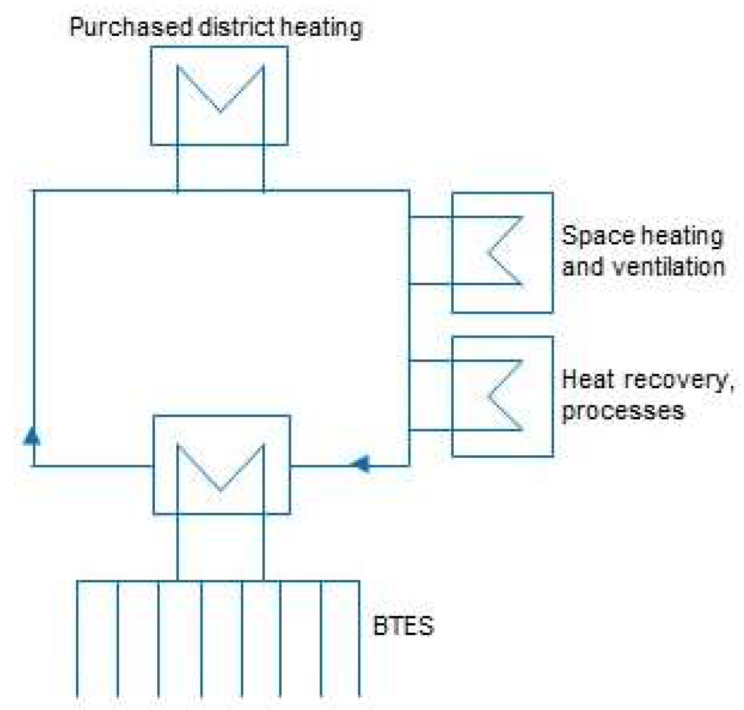
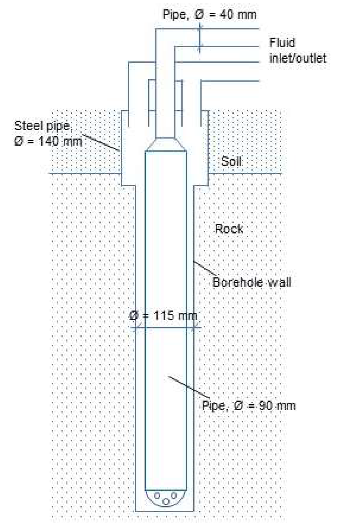
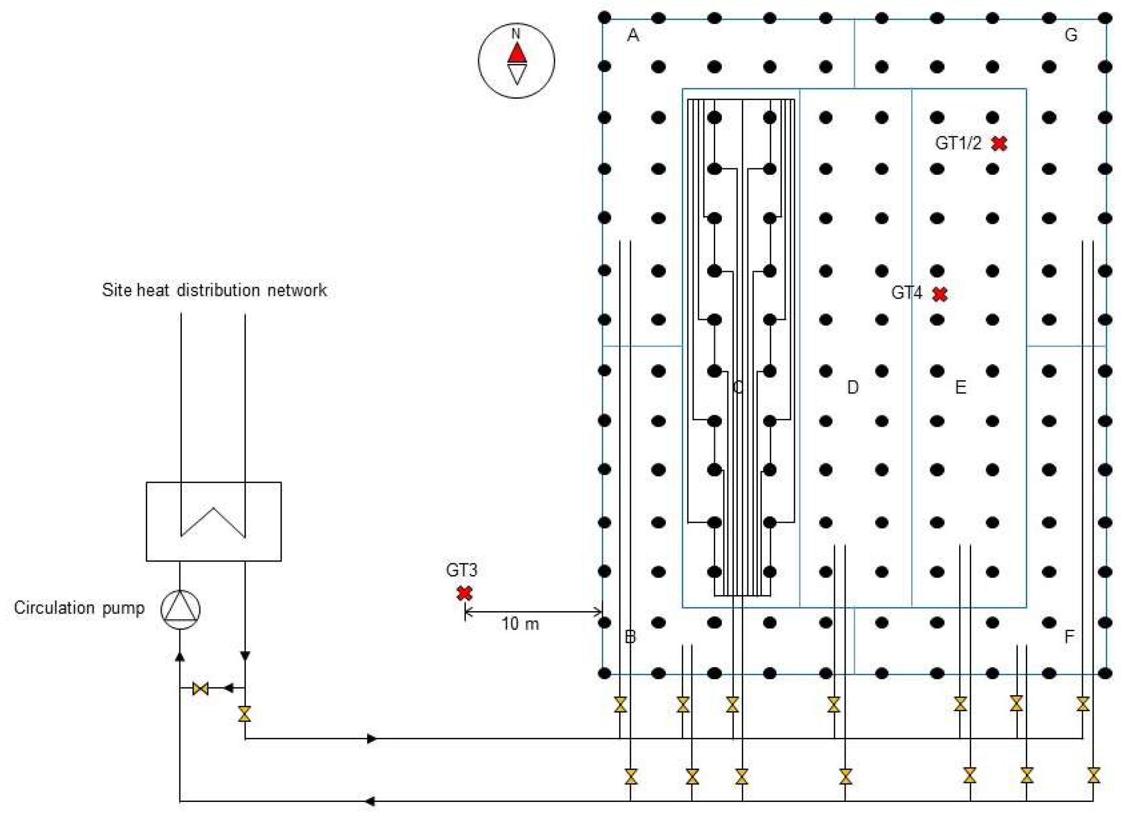
2. Description of the Site and the Modelled BTES

The studied BTES is located at Xylem’s production plant in Emmaboda, Sweden. Xylem, Emmaboda is a manufacturer of submersible pumps and employs roughly 1100 people, of whom 750 work in production. At the site, machine parts are being both assembled and produced. Most of the excess heat comes from a foundry, where approximately 18,000 tonnes of iron are smelted annually, mainly from two high-temperature ovens. The purpose of the BTES is to reduce the site’s purchase of district heating, which is used mainly for ventilation and space heating. Energy is primarily stored in the BTES from summer to winter, but heat is also injected into the storage during times of excess heat in the winter. The heated indoor area at the site measures 110,000 m² and purchased district heating constitutes 4000 MWh/year. A simplified schematic of the site’s heat distribution system is shown in Figure 1.

The BTES, illustrated in Figure 2, consists of 140 boreholes placed in a rectangular array with a borehole spacing and depth of 4 m and 150 m respectively. The storage has been divided into seven sections, A–G, with their own connection to the main supply and return manifold which connect the storage to the site’s internal heat distribution system via a heat exchanger. This partitioning makes it possible to choose which parts of the storage to charge and discharge. For example, at times when excess heat is available at temperatures close to that of the storage centre, it may be injected at the outer partitions where the ground temperature is lower. Each section contains 20 boreholes, connected in series of two and two, as shown in Figure 2 for section C. The flow rate for each section is approximately 3 l/s, meaning a total storage flow rate of about 20 l/s when all the sections are open. Within a section, the flow is distributed equally across the boreholes.

The site’s monitoring system consists of a large number of temperature and pressure sensors, allowing the BTES side of the heat exchanger to operate automatically according to the factory side of the heat exchanger. Ground temperatures are measured by four temperature sensors, GT1–GT4 (see Figure 2). GT1 and GT2 are located within the borehole field at a depth of 117 m and 70 m, respectively. GT3 is located 10 m outside the south-west border of the borehole field at a depth of 100 m, and GT4 is located just beneath the insulation covering the top of the storage. GT1–GT3 are placed in inactive boreholes, used during the design of the storage, whereas GT4 is placed between boreholes. In total, this means that no temperature sensor is in direct contact with the heat transfer fluid. Ground temperatures are measured using Pt100 sensors from Pentronic (four-wire connection, wire wound, class AA according to IEC 60751:2008). With the exception of GT1, for which temperatures are measured every five minutes, ground temperatures are registered every six hours. Energy injected into and extracted from the storage are determined from the mass flow rate and its temperature at the storage entrance and exit. The mass flow rate is calculated from the pressure differential, which is measured using a pressure differential meter from TA Hydronics (TA Link 0-10 V/4-20 mA) with an accuracy of less than 1 kPa. The flow temperatures are also measured using Pt100 sensors from Pentronic. Flow data is registered at five-minute intervals.

The borehole heat exchanger, shown in Figure 3, is of an open type. It consists of a double pipe, a DN 40 pipe inserted into a DN 90 pipe, placed in line with the borehole’s centre point. The heat transfer fluid, being a mixture of groundwater and externally added water, is transported within the DN 40 pipe and the annular space between the DN 90 pipe and the surrounding rock. In the space between the pipes, water is confined by the use of swelling rubber at regular intervals along the borehole heat exchanger length, with the purpose to limit heat transfer between upward and downward flow. The open borehole heat exchanger design is made possible by a nearby dam, which keeps the groundwater level at approximately 2 m beneath ground level year-round. For the distance between ground level and the groundwater table, the borehole is separated from the surrounding rock by a steel pipe. This being considered, and the fact that the pipe system ends at a depth of 146 m, means that the length of the borehole heat exchanger is 144 m. From ground to atmosphere, the surface area confining the boreholes is covered with 0.15 m sand, 0.40 m foam glass, thermal conductivity of 0.11 W/(m·°C), and 0.20 m soil.

Before the construction of the storage, two investigative drillings were made, TH1 and TH2, each to a depth of 150 m [21]. The positions of TH1 and TH2 are given by temperature sensors GT3 and GT1/2 respectively. Rock samples revealed a bedrock primarily made of granodiorite, but with a few 2–5 m layers of amphibolite. The soil depth was determined to be 9 m for TH1 and 5 m for TH2, suggesting a bedrock that dips slightly towards the west. During TH1, a fracture zone with groundwater flow was encountered at a depth of 29–33 m, whilst a minor fracture zone showing groundwater movement was encountered during TH2 near the surface. Through an airlift test, the groundwater flow of the fracture zone in TH1 was determined at 800 l/min.

An illustration of the intermittent storage heat injection and extraction at the site, which occurs as excess heat is also stored in the winter, is shown in Figure 4. Changes between heat injection and extraction mostly occur over the course of a few days. The shortest changes noted are around 10 h.

3. Numerical Procedure

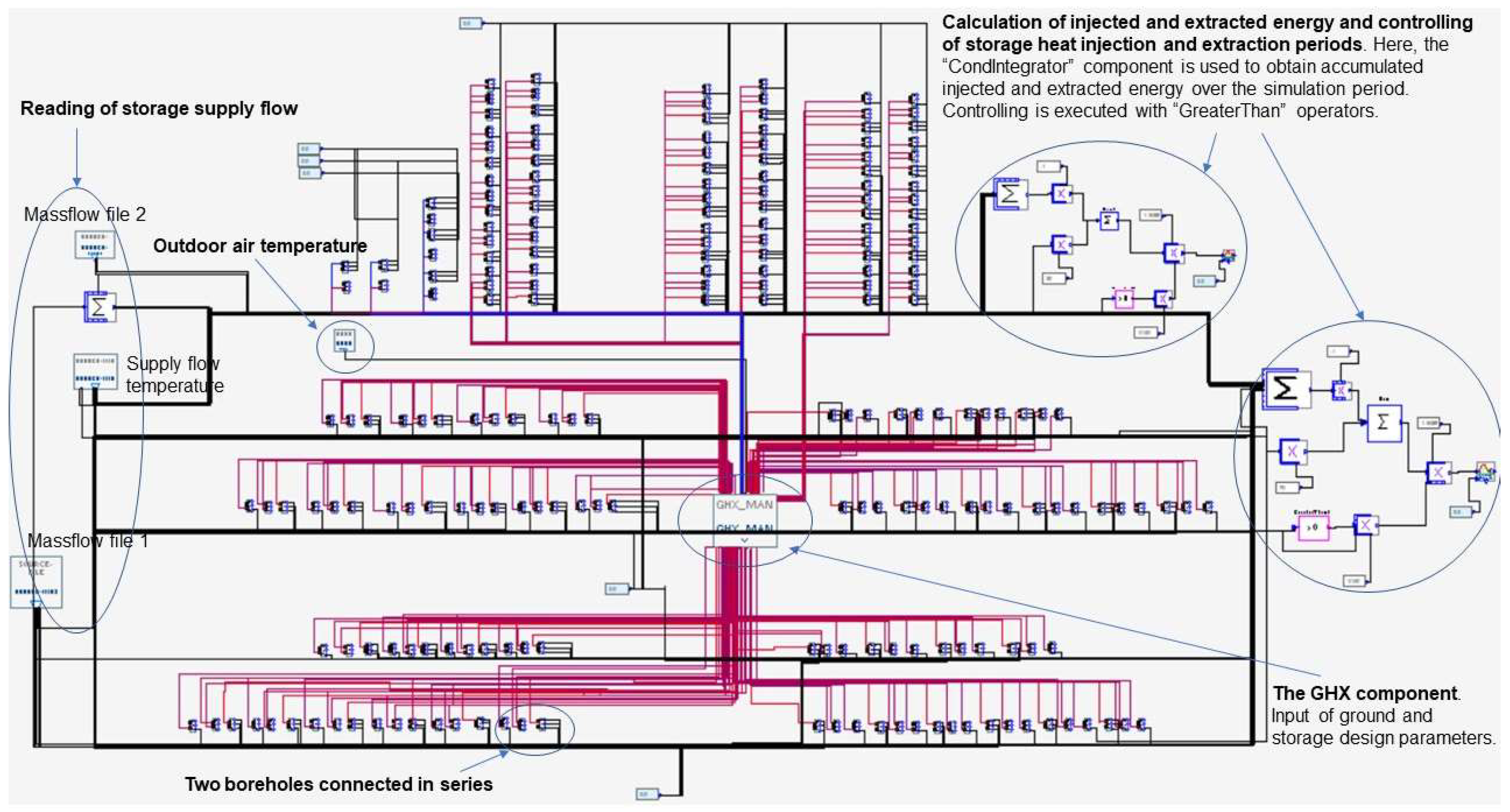
3.1. Numerical Model

IDA ICE 4.8 is a simulation tool that focuses on the dynamic modelling of thermal systems such as heating, ventilation, cooling and generic functions for buildings and industries. IDA ICE is implemented in the general-purpose environment IDA, where all models are available as NMF (Neutral Modelling Format) source code [22]. The simulation environment has been validated and is included in the BESTEST Library [23]. In this study, the IDA ICE GHX module for borehole heat exchangers has been used [24]. The model uses the finite difference method to calculate a 2-D temperature field around each borehole, which are then summed through superposition to generate a 3-D temperature field in the ground. The model can be used for an arbitrary configuration of boreholes of equal depth. The ground is represented by a single layer, but separate properties may be assigned to the top ground layer containing the borehole casing. This means that the ground is modelled using average properties for e.g., thermal conductivity, density and heat capacity. The model is limited to U-pipes as the ground heat exchanger and does not explicitly consider groundwater flow. Boundary conditions for the ground surface is given by the outdoor air temperature, which may vary with time. In the model, the following temperature fields are calculated for each borehole [25]:

• One-dimensional heat transfer between downward and upward flow
• One-dimensional heat transfer between grout (backfill material), liquid and ground
• Two-dimensional heat transfer around the borehole and between the grout and the liquid, using a mesh of cylindrical coordinates

The combined thermal influence on the ground from multiple boreholes is given by superposition. A one-dimensional vertical field, interacting with the ground surface, is used to describe the undisturbed ground temperature. The thermal processes between fluid, grout and borehole wall are dynamic, i.e., the thermal mass of both the fluid and the grout are accounted for. However, the thermal mass of the pipe itself is not considered. To describe the energy balance of downward and upward flow, Equations (1) and (2) [24,25] are applied:

$$\begin{array}{l}M{C}_{p,Liq}·dT{d}_{i,j}/dt\\ =m_i{C}_{p,Liq}·\left(T{d}_{i,j-1}-T{d}_{i,j}\right)+K_{LiqGrout,i}·\left(T_{Groutd,i,j}-T{d}_{i,j}\right)\\ +K_{LiqEarth,i}·\left(T_{i,j}-T{d}_{i,j}\right)\end{array}$$

(1)

$$\begin{array}{l}M{C}_{p,Liq}·dT{u}_{i,j}/dt\\ =m_i{C}_{p,Liq}·\left(T{u}_{i,j+1}-T{u}_{i,j}\right)+K_{LiqGrout,i}·\left(T_{Groutu,i,j}-T{u}_{i,j}\right)\\ +K_{LiqEarth,i}·\left(T_{i,j}-T{u}_{i,j}\right)\end{array}$$

(2)

where $M{C}_{p,Liq}$ (J/°C) is the absolute heat capacity of the upward or downward flow in node $j$ at borehole $i$, $T{d}_{i,j}$ (°C) and $T{u}_{i,j}$ (°C) are the temperature of the downward and upward flow respectively in node $j$ at borehole $i$, $m_i$ (kg/s) is the mass flow rate at borehole $i$, $C_{p,Liq}$ (J/(kg·°C)) is the specific heat capacity of the fluid at borehole $i$, $K_{LiqGrout,i}$ (W/°C) is the heat transfer coefficient multiplied by area between grout and fluid at borehole $i$, $T_{Groutd,i,j}$ (°C) and $T_{Groutu,i,j}$ (°C) are the grout temperature around the downward and upward flow respectively in node $j$ at borehole $i$, $K_{LiqEarth,i}$ (W/°C) is the heat transfer coefficient multiplied by area between the fluid and borehole wall at borehole $i$, and $T_{i,j}$ (°C) is the borehole wall temperature in node $j$ at borehole $i$.

The energy balance of the filling material is described by Equations (3)–(5) [24,25]:

$$\begin{array}{l}M{C}_{p,Grout2 }·d{T}_{Grout,i,j}/dt\\ =K_{GroutGrout}·\left(T_{Groutd,i,j}- T_{Groutu,i,j}-2T_{Grout,i,j}\right)\\ +K_{GroutEarth}·\left(T_{i,j} -T_{Grout,i,j}\right)\end{array}$$

(3)

$$\begin{array}{l}M{C}_{p,Grout1 }·d{T}_{Groutd,i,j}/dt=K_{GroutGrout}·\left(T_{Grout,i,j}- T_{Groutd,i,j}\right)+ \\ K_{LiqGrout,i}·\left(T{d}_{i,j} -T_{Groutd,i,j}\right)+K_{RingEarth}·\left(T_{i,j}-T_{Groutd,i,j}\right)\end{array}$$

(4)

$$\begin{array}{l}M{C}_{\left(p,Grout1\right)}\cdot d{T}_{Groutu,i,j}/dt=K_{GroutGrout}\cdot (T_{Grout,i,j}-T_{Groutu,i,j})\\ +K_{LiqGrout,i}\cdot (T{d}_{i,j}-T_{Groutu,i,j})+K_{RingEarth}\cdot (T_{i,j}-T_{Groutu,i,j})\end{array}$$

(5)

where $M{C}_{p,Grout2 }$(J/°C) and $M{C}_{p,Grout1 }$(J/°C) are the absolute heat capacity of the outer and inner grout respectively, $T_{Grout,i,j}$ (°C) is the temperature of the outer grout in node $j$ at borehole $i$, $K_{GroutGrout}$ (W/°C) is the heat conductivity coefficient multiplied by length between the grout ring and outer grout, $K_{GroutEarth}$ (W/°C) is the heat conductivity coefficient multiplied by length between grout and ground, and $K_{RingEarth}$ (W/°C) is the heat conductivity coefficient multiplied by length between grout ring and ground.

Heat resistances used to calculate the heat conductivity coefficients, $K$, are either entered directly or calculated by providing an effective borehole thermal resistance, $R_b$. The effective borehole thermal resistance, $R_b$ is the thermal resistance between the heat transfer fluid and the borehole wall, assuming a steady-flux state [26]. A more detailed description of the model is found in [24].

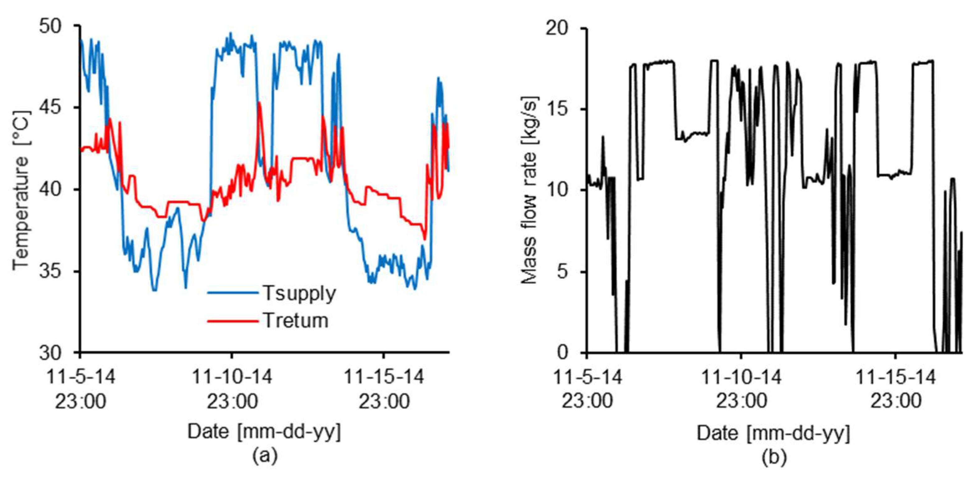
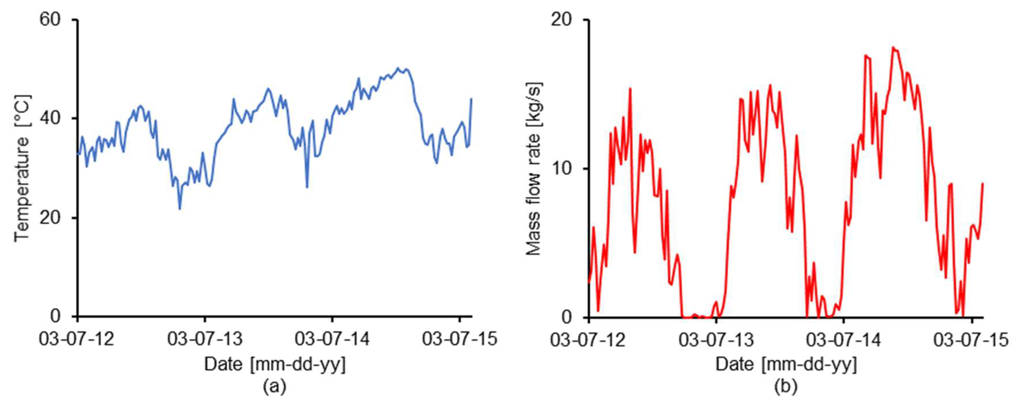
3.2. The Modelled System and Validation Setup

For model validation, values for the energy injected into and extracted from the storage were used, along with ground temperatures, measured by temperature sensors GT1–GT4 (see Figure 2). For the validation period considered, March 2012–March 2015, the maximum measurement error of the average storage supply flow, 12.6 l/s, was determined at 4.9%. The maximum measurement error for the mean storage supply (37.5 °C) and return flow temperature (35.3 °C) are 0.8% and 0.9% respectively. By considering average values for temperatures and flow, the maximum error is 12.9% for registered injected energy and 16.5% for registered extracted energy. At the mean values measured by ground temperature sensors GT1–GT4, 19.3–33.6 °C, the maximum measurement error is in the range 0.9–1.6%.

An uncertainty when modelling any BTES is the ground properties, along with the effective borehole thermal resistance. Here, simulations were carried out for various values of the effective borehole thermal resistance, whilst the effective ground thermal conductivity and ground volumetric heat capacity were kept at fixed values. Values for the effective borehole thermal resistance were limited to 0.05, 0.10, and 0.15 (m·°C)/W, based on a value of 0.10 (m·°C)/W being common for these applications [27]. Good agreement between the modelled and measured data was achieved when $R_b$ was set to 0.15 (m·°C)/W. Based on ground samples taken prior to the construction of the storage, showing a ground composition primarily made up of reddish grey to light grey granodiorite [21], the volumetric heat capacity was set to 2.2 MJ/(m³·°C). The effective ground thermal conductivity was set to 6 W/(m·°C), which was obtained when it was calculated from measured ground temperatures using steady-state heat transfer through cylindrical shells, see Equation (6) [28]:

$$\dot{Q}=2\mathsf{\pi }\mathrm{kL}\frac{T1-T2}{\ln (r2/r1)}$$

(6)

where $\dot{Q}$ is the heat transfer rate (W), $\mathrm{k}$ is the ground thermal conductivity (W/(m·°C)), $\mathrm{L}$ is the cylinder length (m), $r1$ and $r2$ are the inner and outer radius respectively (m), and $T1$ and $T2$ are the respective temperatures at these positions (°C). In this case, the cylinder of radius $r1$ is represented by a cylinder of approximate volume and surface area as the volume confining the borehole field, limited in height by the positions of GT2 (70 m) and GT1 (117 m). The temperature $T1$ of this cylinder is given by the average value of GT1 and GT2. The radius $r2$ is given by the distance between the borehole field centre and the position of GT3. $T2$ is given by the temperature of GT3. Calculations consider the average heat transfer rate $\dot{Q}$, which is obtained from the change in temperature of the cylinder of radius $r1$, and the average temperature difference $T1$–$T2$ for periods of heat injection only, i.e., summer. This calculated value of 6 W/(m·°C) can be compared to the ground thermal conductivity of only granodiorite, approximately 2.7 W/(m·°C) [29], which does not consider e.g., possible fracture zones with groundwater movement at the storage location.

As IDA ICE GHX is limited to closed-loop borehole heat exchangers, the open borehole heat exchanger was modelled as a single U-pipe. The inner radius of the U-pipe was set to 16 mm, and water was used as backfill material. The used properties of water was 4.18 kJ/(kg·°C) for specific heat, 1000 kg/m³ for density and 0.6 W/(m·°C) for thermal conductivity. The borehole diameter was set to the same as for the actual case (115 mm). The unaffected ground temperature was set to 8 °C, as determined from site investigations [21]. The distance between the surface level (0 m) and the beginning of the ground heat exchanger (approximately −2.8 m) was modelled as one layer with the weighted average properties of the individual layers. The outdoor air temperature for the period considered was taken from a nearby weather station, located in Kosta, Sweden. In the model, boreholes were connected in series of two and two, according to the real case.

The storage came into operation in June 2010, but data for the injected and extracted energy and ground temperatures were first measured in March 2012. The model was initiated to correspond to the starting conditions. However, the temperature measured by GT4 is strongly affected by the outdoor climate as the sensor is placed just below the top insulation of the storage. The operation of the storage at heat extraction was limited to the three inner storage sections, which resembles the actual operation of the storage where this most of the time has been the case. For heat injection, which primarily takes place with four and five storage sections open, the operation of the storage was approximated by letting the flow be evenly distributed across all the boreholes. The measured storage supply flow data, used as model input, is shown in Figure 5. In the model, a resolution of one hour was used for the storage supply flow data.

The model layout is shown in Figure 6. The component at the centre is the IDA ICE GHX component, where such aspects as geological and storage design parameters are assigned. The arrays of components are borehole inlets and outlets, where each group of 30 components corresponds to one of the storage sections A–G. Each set of three components corresponds to two boreholes connected in series, where the first component gives the inlet of the first borehole, the second component the outlet of the first borehole and the inlet of the second borehole, and the third component the outlet of the second borehole. Storage supply flow data is supplied to the borehole inlets from the components on the far left. In order to control the storage operation in the model validation so that heat extraction is limited to sections C–E, one input file is used to supply the mass flow rate to sections C–E and another to the remaining sectors. For the parametric study, presented in detail below, the mass flow rate supplied to the storage is given by the sum of the two input data files. In this case, one of the files represents heat injection and contains non-zero values for the mass flow rate during times of heat injection and zero values during times of potential heat extraction, whereas, the opposite is true for the other file, which represents heat extraction. At the beginning of each simulation time step, the input file corresponding to heat extraction will be multiplied by the number 1 in cases where the storage return flow temperature from the previous time step exceeds the minimum useful storage temperature and otherwise it will be multiplied by 0. This logical operation takes place to the right in the figure, where the injected and extracted energy are also calculated.

3.3. Parametric Study

For the parameterization, the impact on storage performance in terms of injected and extracted energy was investigated for various storage supply flow characteristics at heat injection, borehole spacings, borehole depths, ground thermal conductivities, and minimum useful storage temperatures. The analysis of ground thermal conductivity and minimum useful storage temperature is limited to the actual storage supply flow at heat injection. Parameterization of borehole spacing and borehole depth was carried out for six different combinations of the storage supply flow at heat injection, being multiples of the actual supply flow. The combinations were chosen with the purpose of investigating the influence of storage performance from storage supply flow temperature as well as storage supply flow rate. These combinations are denoted as Cases 1–6 and are presented together with their corresponding annual absolute mean values in

Table 1. Combinations of the storage supply flow at heat injection considered in the parametric study, Cases 1–6. Bold print denotes the actual flow (Case 6). Mass flow rate (kg/s) and flow temperature (°C) are annual mean values.

Case	Mass Flow of Actual (%)	Flow Temperature of Actual (%)	Mass Flow Rate (kg/s)	Flow Temperature (°C)
Case 1	75	200	10	80
Case 2	150	150	20	60
Case 3	100	150	13	60
Case 4	75	150	10	60
Case 5	150	100	20	40
Case 6	100	100	13	40

. Case 6 is the actual storage supply flow at heat injection. Parameters considered in the study and their ranges are presented in

Table 2. Parameters and parameter ranges considered in the sensitivity analysis of the borehole thermal energy storage (BTES) performance. Bold print denotes actual design and geological values for the BTES at Xylem, Emmaboda.

Parameter	Values	Case
Borehole spacing (m)	1, 2, 3, 4, 5, 6, 7, 8	1–6
Borehole depth (m)	84, 114, 144, 174, 204, 234, 264, 294, 324	1–6
Modelled ground thermal conductivity (W/(m·°C))	1, 2, 3, 4, 5, 6, 7, 8	6
Minimum useful storage temperature (°C)	30, 35, 40, 45	6

. Also, the parameter values are based on the actual values at the site.

Calculations assume that heat extraction takes place during the building heating season whenever heat is not injected and the storage can deliver the minimum useful temperature to the internal heat distribution network. A supply flow temperature of a minimum of 40 °C is required to be supplied to the internal heat distribution network for existing heat exchangers. It is assumed that all extracted energy is useful. Heat extraction takes place at maximum flow rate, which for Cases 1–5 is scaled from the actual maximum storage flow rate, Case 6, in accordance to the flow rate at heat injection. The flow is distributed evenly across all the boreholes both at heat injection and extraction. For Emmaboda, the building heating season is September 15 to May 15.

Simulations were conducted for a long enough time for the storage to reach an annual steady state, i.e., storage performance is repeated for subsequent years. For the time after the end of the measured data, March 2015, the previous year’s storage supply flow data at heat injection was repeated for each following year. Annual steady state was considered to have been reached when the yearly injected energy for the next year changed by less than 5% and the ground temperatures as given by GT1–GT4 at the start and end of the years differed by 1 °C or less and showed similar patterns throughout the year. The annual steady-state criterion is illustrated in Figure 7, by considering one ground temperature point. In Figure 7, the annual steady state is considered to have been reached in year six. From when annual storage supply flow data at heat injection was repeated, the yearly steady state was reached in between two and four years in all cases. Based on findings from the model validation, presented later, parameterization was conducted using daily averages for the supply flow data used as model input. The remaining model input parameters are the same as for the validation.

4. Results and Discussion

This section will start with the three-year comparison of calculated and measured storage performance, including a time-step dependency analysis for calculated storage performance. This will then be followed by the results of the parametric study, starting with the influence of borehole spacing on storage performance, followed by the influence of borehole depth, ground thermal conductivity, and minimum useful storage temperature.

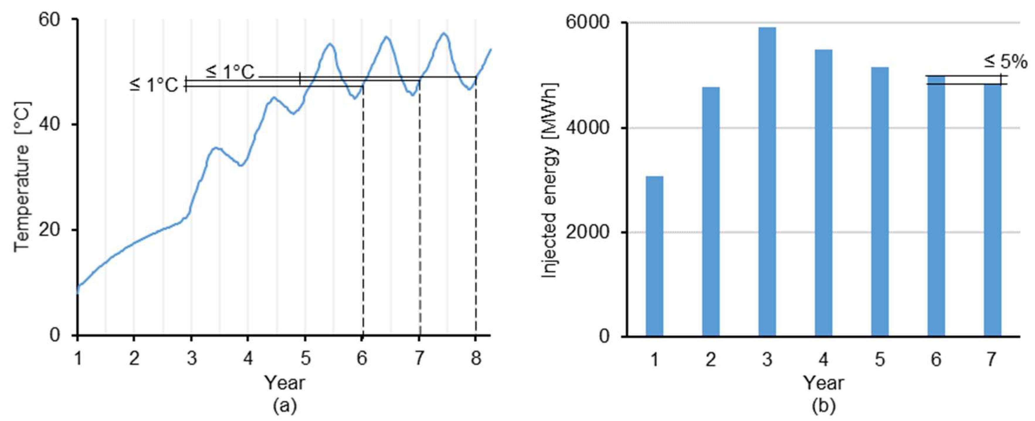
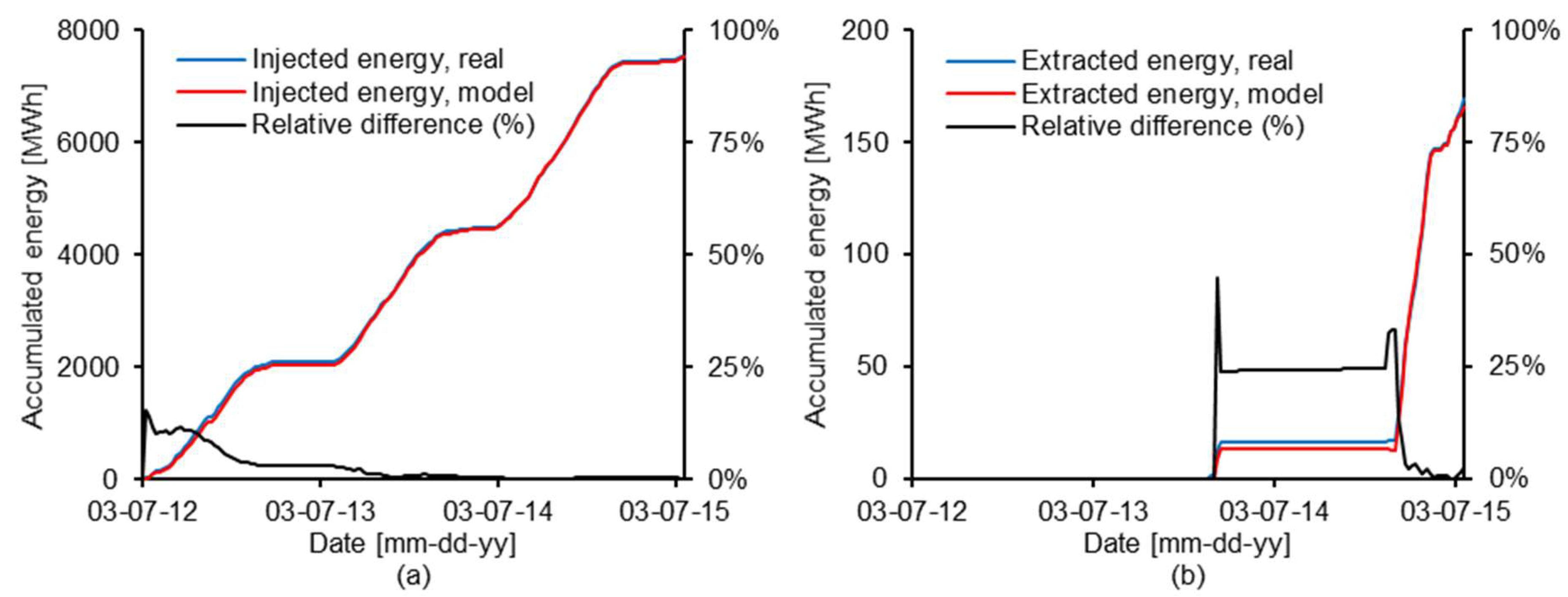
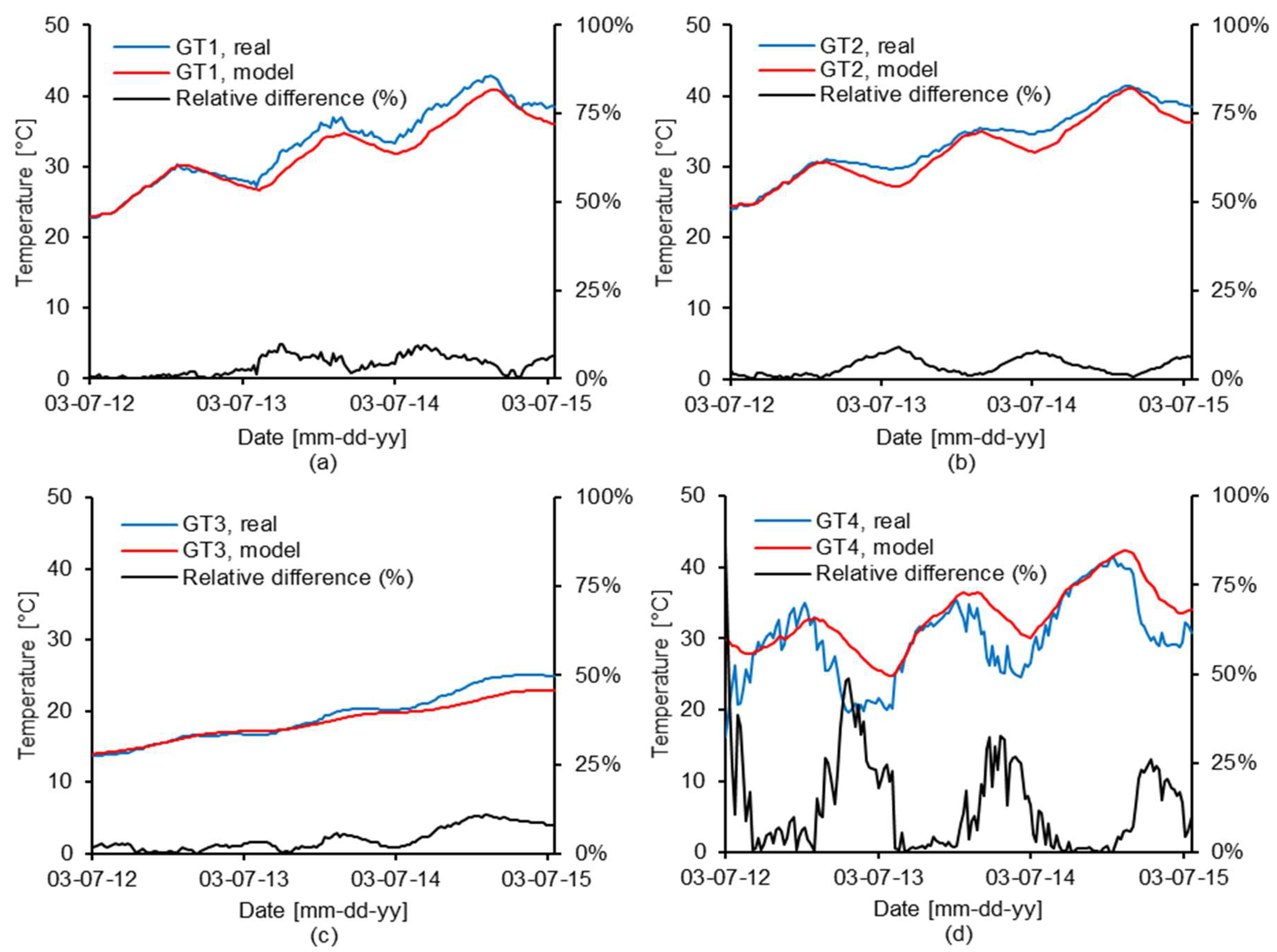
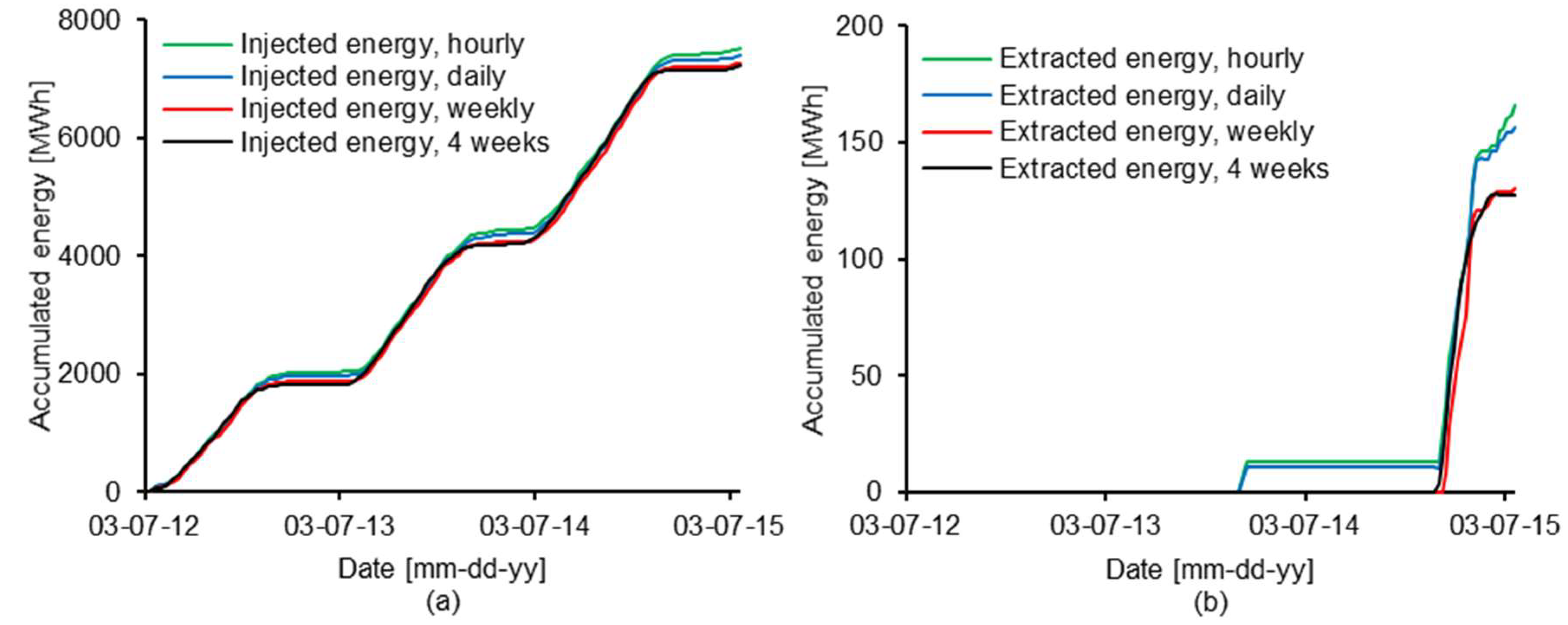
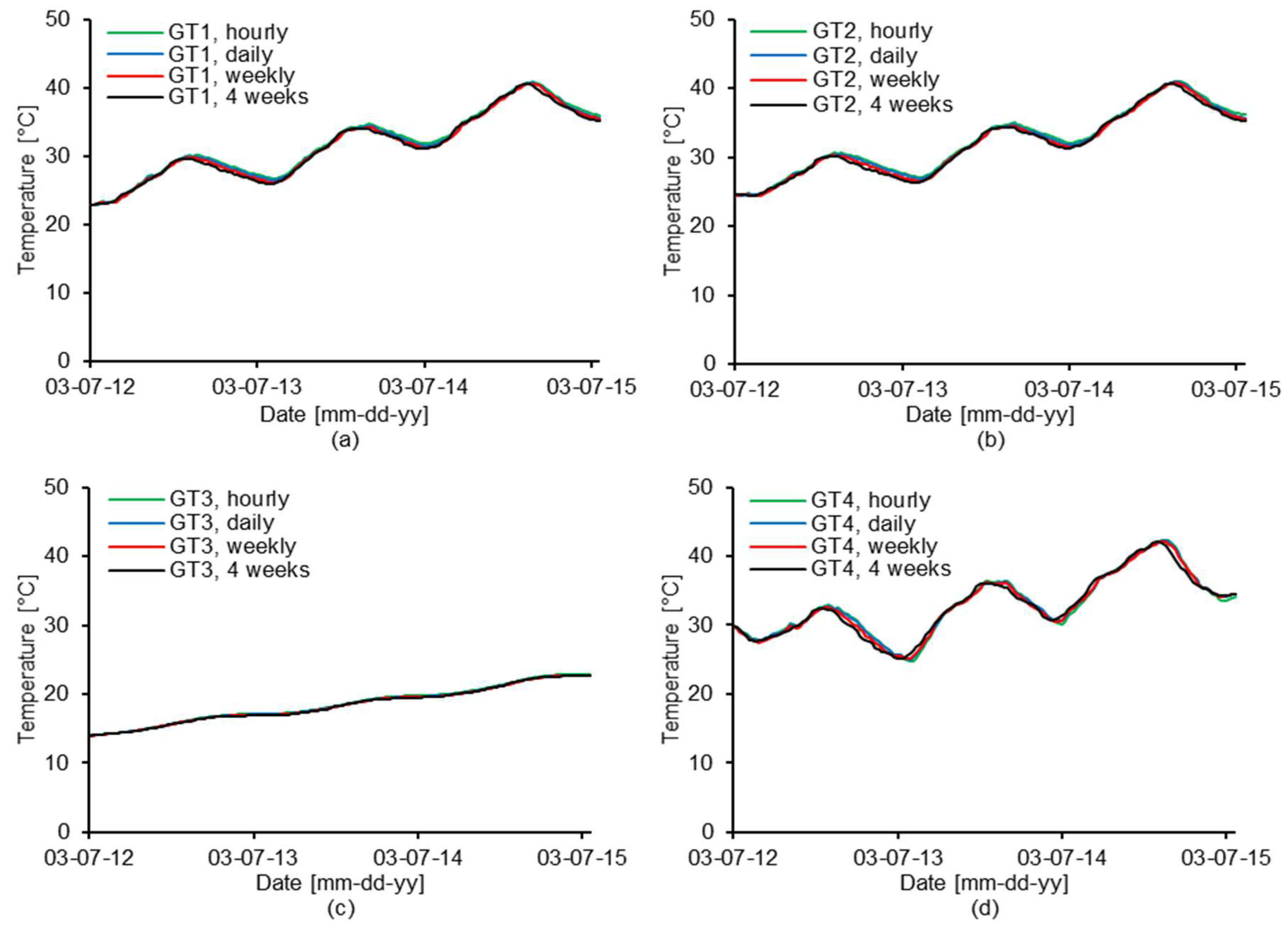
4.1. Model Validation and Time-Step Dependency

For injected and extracted energy, the predicted values deviate from measured values by less than 1 and 3%, respectively, for the three-year comparison, and curves for predicted and actual values follow the same pattern (Figure 8). The same patterns between modelled and measured values are also seen for the ground temperatures (Figure 9). Both for GT1, GT2, and GT3, which are all located at depths of between 70 and 117 m, the mean relative difference between modelled and measured data for the period is 4%, and for GT4, located just beneath the insulation covering the top surface of the borehole field, the mean relative difference is 13%. Both for calculated and measured data, the BTES efficiency for the whole period is 2%. The reason why the BTES efficiency and extracted energy are not higher is because extraction is limited by the return flow temperature at the internal heat distribution network, which during the winter is 35–40 °C. A BTES system often needs a few years before reaching high enough temperatures to allow heat extraction to take place. But, as shown by Catolico et al. [15], the performance of a BTES system may also continue to increase with time due to changed boundary conditions for subsequent cycles because not all of the injected energy is recovered on each cycle.

The larger temperature changes seen for the modelled values of GT2 compared to the measured values suggest a ground composition at this location that has a higher heat capacity than that used for the ground in the model. Although site investigations showed a bedrock primarily made of granodiorite, it also showed some 2–5 m thick layers of amphibolite, which has slightly higher heat capacity than that of granodiorite. For ground formations, geological properties may be different at different depths. For example, dependent on e.g., porosity and water content, the ground thermal conductivity can range from around 1 W/(m·°C) up to 7 W/(m·°C), showing the importance of site investigations prior to the construction of the BTES. For GT4, the temperature difference between the modelled and measured values as of March 2012 is almost 15 °C and the slower temperature changes seen for the modelled data suggest that the climate has a smaller impact on GT4 in the model. Reasons for this could be an overprediction of the thermal resistance of the layer above the borehole heat exchangers, as well as climate data limited to outdoor temperature. For example, heat transport from the region could be affected by rain permeating the ground. On the other hand, the difference in temperature at GT4 has little effect on storage performance. One-dimensional steady-state heat conduction through the layer covering the borehole field, from the position of GT4 to the atmosphere, gives a storage heat loss of 255 and 225 MWh respectively for modelled and measured temperatures for the three-year period, i.e., ca 3% of the total injected energy.

In Figure 10 and Figure 11, model output for an hourly time step is compared to the output obtained using a time step of one day, one week, and four weeks. Apart from extracted energy, the choice of time step barely affects the model output. Differences seen for extracted energy can be explained by the at times rapid changes between storage heat injection and extraction, occurring at intervals of between half a day and a few days. These short-term changes in storage operation are lost when supply flow data is averaged over periods longer than those at which they occur. The simulation time was approximately 40 h, 5 h, 40 min, and 15 min for a time step of one hour, one day, one week, and four weeks respectively. Simulations were carried out using an Intel Xeon processor (3.70 GHz, four cores), a SSD with 1800 MB/s write speed, and 16 GB of RAM.

4.2. Parametric Study

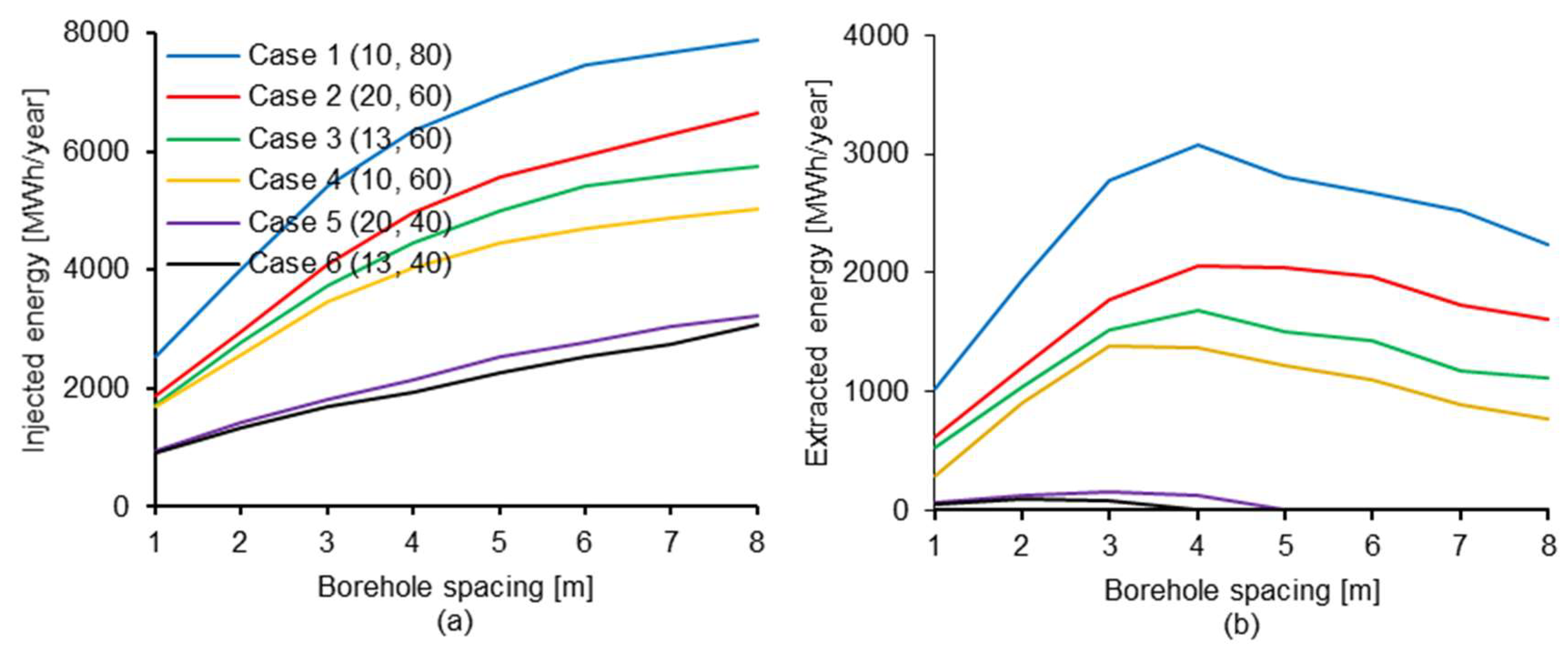
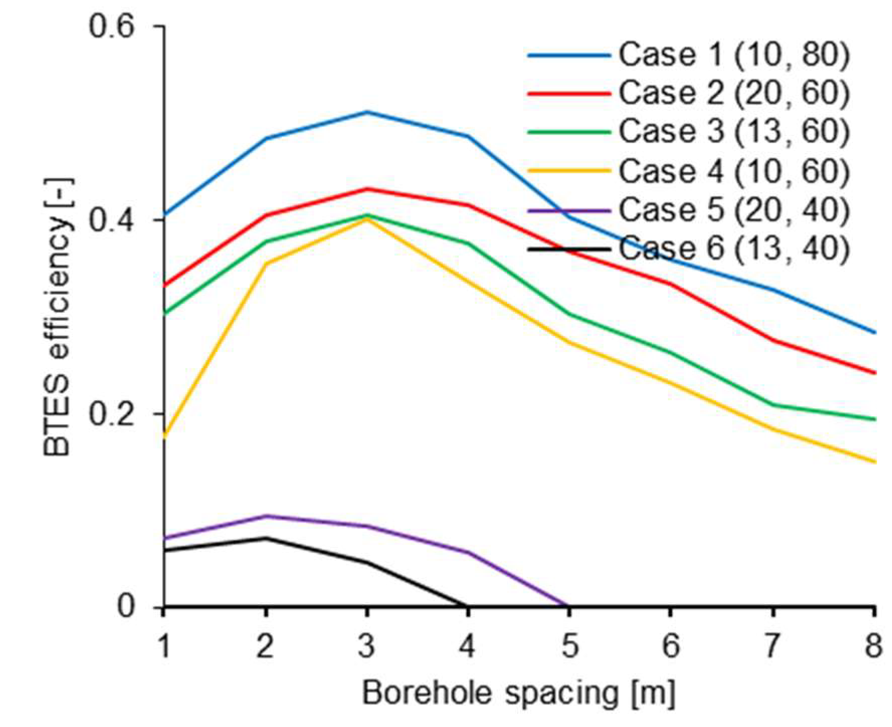
4.2.1. Borehole Spacing

A key parameter for BTES is the borehole spacing because this will affect the volume into which heat is injected and the degree to which the boreholes thermally interact with each other. In Figure 12, annual heat injection and extraction for the storage at Emmaboda are shown as function of borehole spacing for the six constructions of the supply flow at heat injection, Cases 1–6. For all flows, the amount of energy that can be injected into the storage increases with increasing borehole spacing. This outcome is expected because an increased borehole spacing means that energy is injected into a larger ground volume, i.e., the thermal mass of the volume confining the boreholes is increased, resulting in a higher temperature difference between the ground and the heat transfer fluid. It is visible that the change in injected energy for each increment in borehole spacing decreases as the spacing becomes larger. The curve will continue to flatten out as the heat transfer process around a borehole from an increased borehole spacing approaches a state where it is negligibly affected by any other borehole. From a spacing of 7 to 8 m, injected energy increases by 3–6% for considered flows. For all flows, a logarithmic curve fit gives an increase in annual injected energy for each increment (1 m) in borehole spacing of less than 2% and 1% when the borehole spacing reaches approximately 15 and 25 m respectively.

If the borehole spacing is too large, the storage will not reach high enough temperatures for heat to be extracted, and a spacing that is too small means that potential heat that could be stored and recovered is lost. The existence of an optimum borehole spacing for heat extraction is in line with the findings of Welsch et al. [30]. In this case, a borehole spacing of 4 m yields the highest heat extraction for Cases 1–3, whilst 3 m gives the highest value for Case 4. At these spacings, 3080, 2060, 1680, and 1380 MWh/year can be extracted for Cases 1, 2, 3 and 4, respectively. Overall, the reduction in extracted energy is higher when the spacing is decreased than increased from this point. For Cases 1–3, more energy can be extracted at a spacing of 8 m than 2 m. For the considered flows, the energy that can be injected and extracted at the same borehole spacing is in descending order first related to the flow temperature and secondly to the flow rate. The actual flow temperature, Cases 5 and 6, is not sufficient for the storage to reach the temperatures necessary for any noticeable amount of energy to be extracted.

However, for Cases 1–4, extracted energy at larger borehole spacings could be increased by increasing the flow rate or only using the inner boreholes. This is demonstrated for Case 2 in Figure 13, which shows the horizontal temperature distribution at half the borehole depth (72 m) for Case 2 when the temperatures within the borehole field at this line are at their annual maximum and minimum, respectively. From the area between the black line, indicating minimum useful ground temperature, and the minimum temperature graphs, it can be seen that when the borehole spacing increases there is an increasing amount of energy that is never extracted. This can be explained by the lower storage temperatures with a larger borehole spacing, meaning a lower temperature difference between the ground and the heat transfer fluid and thus lower power output.

The ratio of heat extracted to heat injected, known as the BTES efficiency, is shown for Cases 1–6 as a function of borehole spacing in Figure 14. As for heat extraction, the highest values are obtained at a moderate borehole spacing. Although a larger volume taken up by the borehole field often means a higher volume-to-area ratio of the borehole field and lower relative heat losses to the surroundings, the storage needs to reach high enough temperatures in order to reach high heat extractions and efficiencies. In this case, part of the lower efficiency at larger borehole spacings is explained by the non-extracted energy, Figure 10. For Cases 1–3, the highest BTES efficiency is achieved at a borehole spacing of 3 m, although most energy can be extracted at a spacing of 4 m. However, their respective efficiencies are almost the same at a spacing of 3–5 m. For Cases 1–4, efficiencies reach 40–50%, whilst efficiencies for Cases 5 and 6 do not exceed 10%.

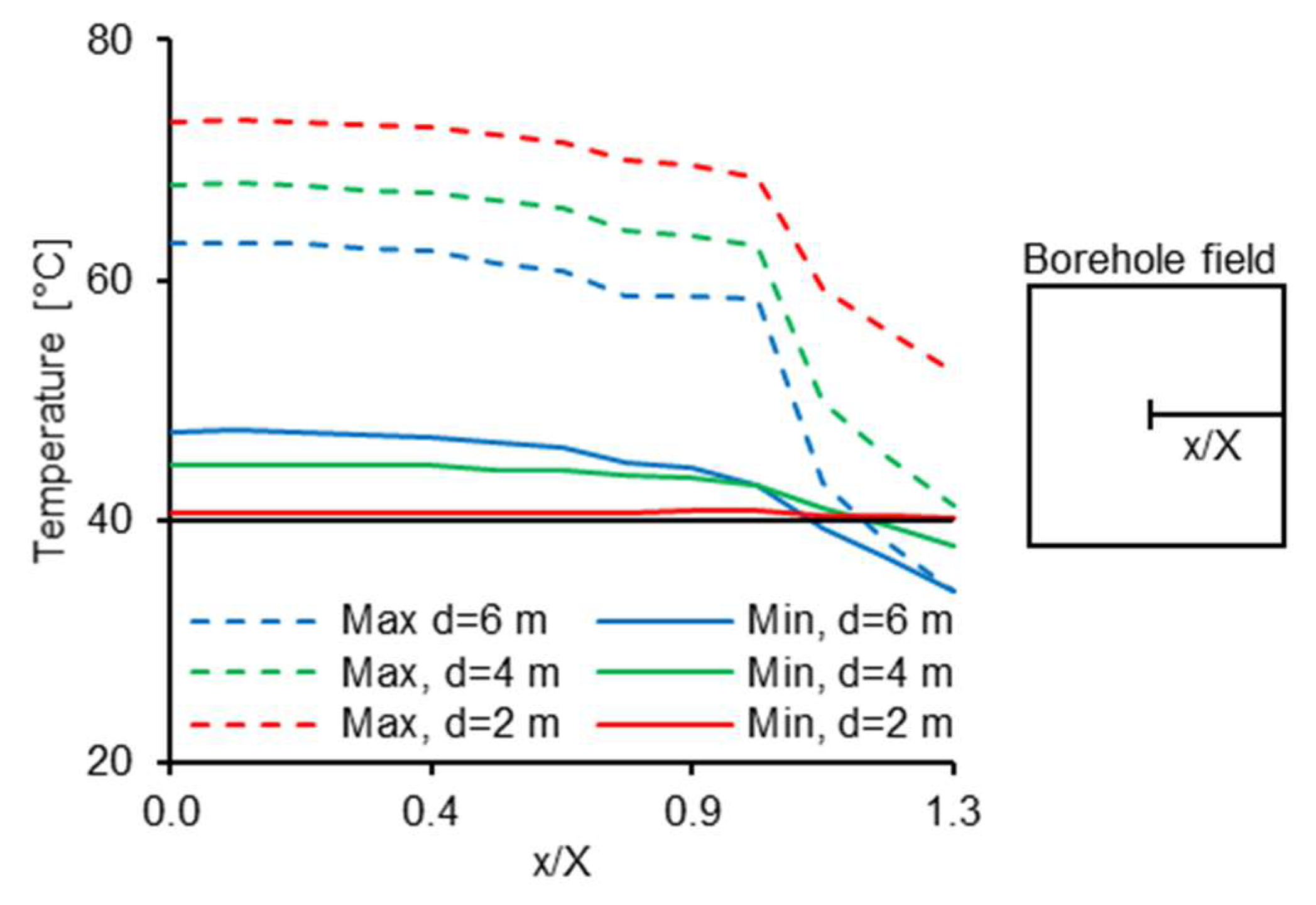
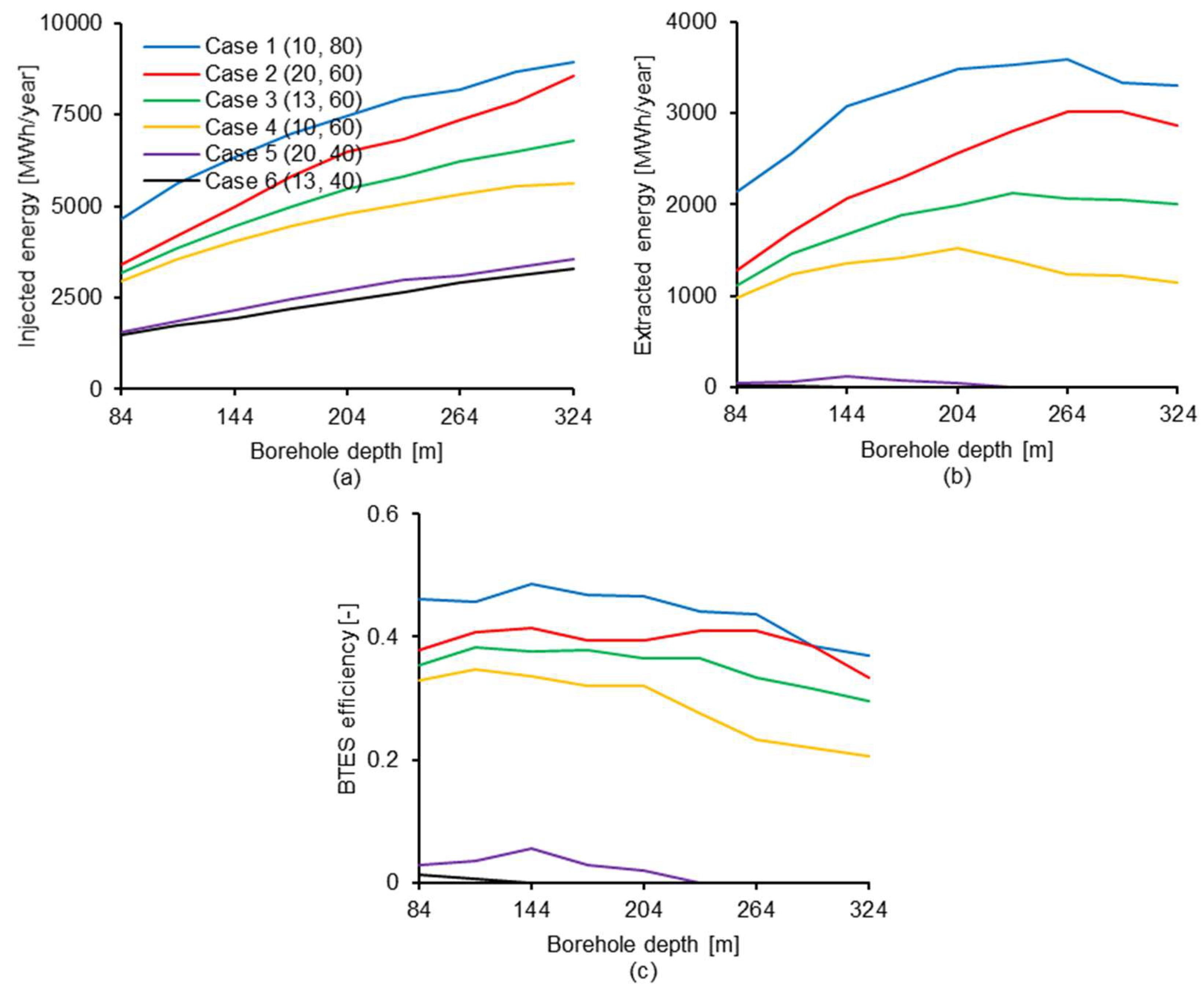
4.2.2. Borehole Depth

As with borehole spacing, borehole depth will affect the volume into which heat is injected, but also the heat exchange length between the heat transfer fluid and the ground. In Figure 15, it can be seen that from a borehole depth of 84 m; the injected energy increases almost linearly for all flows with the extended borehole heat exchanger length from an increased borehole depth. However, this increase per metre of borehole depth is lower than the average heat injection per metre until a borehole depth of 84 m, as seen from the graphs’ starting points, meaning that heat injection per metre of borehole decreases with borehole depth. The basis for this is that the storage supply flow temperature at heat injection is at its highest at the borehole inlet, for example facilitating heat transfer between the fluid and the ground closer to this point. The lower heat injection with increased depth results in lower storage temperatures and gives a cut-off point of borehole depth for heat extraction. For Cases 1 and 2, this cut-off point takes place soon after a borehole depth of 264 m, whilst the extracted energy has already begun to decline after a depth of 234 m for Case 3 and after 204 m for Case 4. At these depths yielding the highest annual heat extraction, 3590, 3020, 2130, and 1530 MWh/year can be extracted for Cases 1, 2, 3, and 4 respectively. For Cases 1–3, the respective BTES efficiencies are almost the same between the depths of 84 and 234 m. The BTES efficiency may be a good indicator for how well a certain BTES performs but does not disclose whether for a given heat load the BTES could have been designed differently so that higher heat extractions could have been achieved. Moreover, if there is a warm winter, the BTES efficiency may be limited by the site’s heat demand, resulting in a lower efficiency than could otherwise have been achieved. This was reported for the BTES at the Drake Landing Solar Community [15].

By comparing Figure 15 to Figure 12, it can be seen that apart from Cases 5 and 6, for which heat extraction is very small, more energy can be extracted from increasing the borehole depth than by altering the borehole spacing. The percentage increase is largest for the case having the highest mass flow rate, Case 2, where 47% more energy can be extracted at the best-performing borehole depth in this aspect as compared to the best-performing spacing. A benefit of deeper boreholes is the longer heat exchanger length obtained for the same volume taken up by the borehole field as compared to shallower boreholes. On the other hand, deeper boreholes will in general mean a lower volume-to-area ratio of the borehole field, increasing relative heat losses from the borehole field to the surroundings. It should also be noted that in practice ground heat exchanger installations rarely exceed a depth of around 250 m due to the difficulty and cost of drilling at these depths. As for the investigation of borehole spacing, extracted energy is in descending order first given by the flow temperature and secondly by the flow rate.

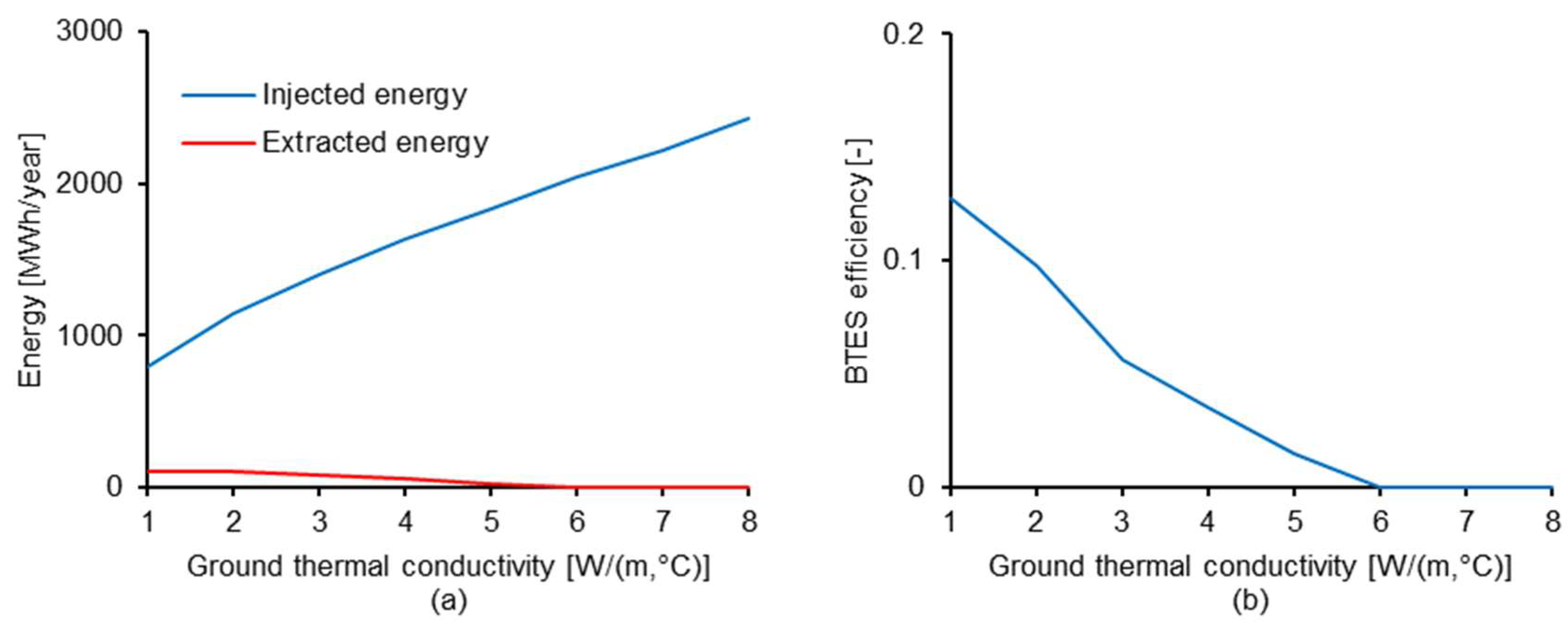
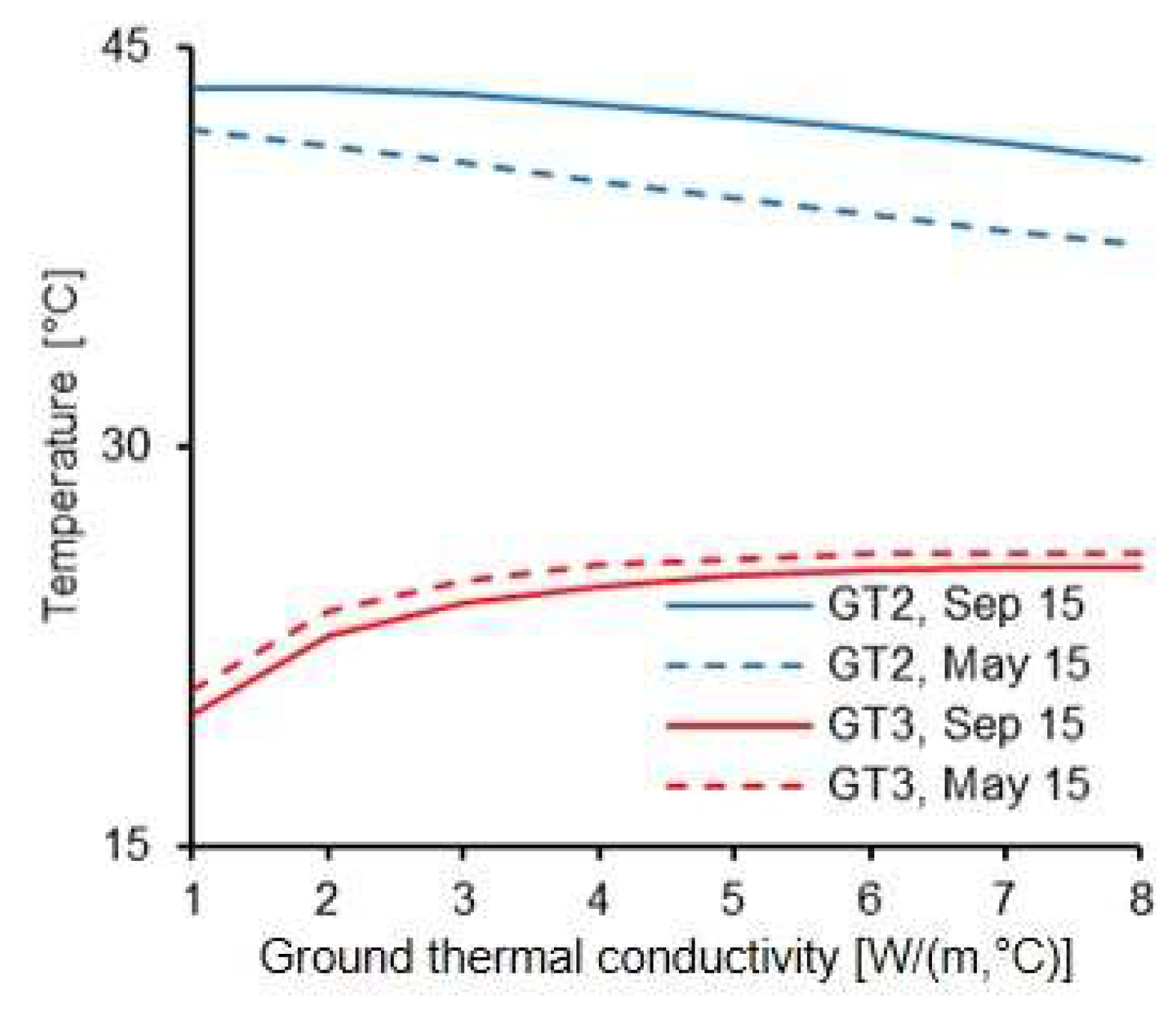
4.2.3. Ground Thermal Conductivity

A crucial parameter for the heat transfer process in the ground in the presence of a BTES is the (effective) ground thermal conductivity. In Figure 16, ground thermal conductivity is plotted against annual injected and extracted energy and BTES efficiency at annual steady state for the actual storage design and supply flow at heat injection, Case 6. It can be seen that, independent of ground thermal conductivity, only a small amount of energy can be extracted, at most around 100 MWh/year. The lower retention of heat at the boreholes for a higher ground thermal conductivity is seen from the increasing amount of energy that can be injected. In either case, however, temperatures at the borehole field, given by GT2, Figure 17, are barely affected by the ground thermal conductivity. Presently, storage temperatures above 40 °C are considered useful. If heat were extracted at lower storage temperatures so that storage temperatures were not as close to the supply flow temperature at heat injection, Figure 5, it is likely that the impact on heat extraction as a function of ground thermal conductivity would be more significant. However, the results shown in Figure 16 support the concept of Başer et al. [5] that a BTES system installed in unsaturated ground formations may achieve higher performances than a BTES system installed in saturated ground formations, because of the lower ground thermal conductivity of the former. It should be noted for the temperature graphs for May 15 in Figure 17 that some heat is also injected between September 15 and May 15.

From GT3, located 10 m from the storage border at a depth of 100 m, it can be seen how the increase in temperature levels out with increasing ground thermal conductivity according to the logarithmic behaviour of heat transfer taking place radially, which was an expected outcome. The reason that around 170 MWh of heat could be extracted during the winter of 2014–2015 at a ground thermal conductivity of 6 W/(m·°C) in the model validation, Figure 8, is due to heat extraction in that case was limited to the inner boreholes.

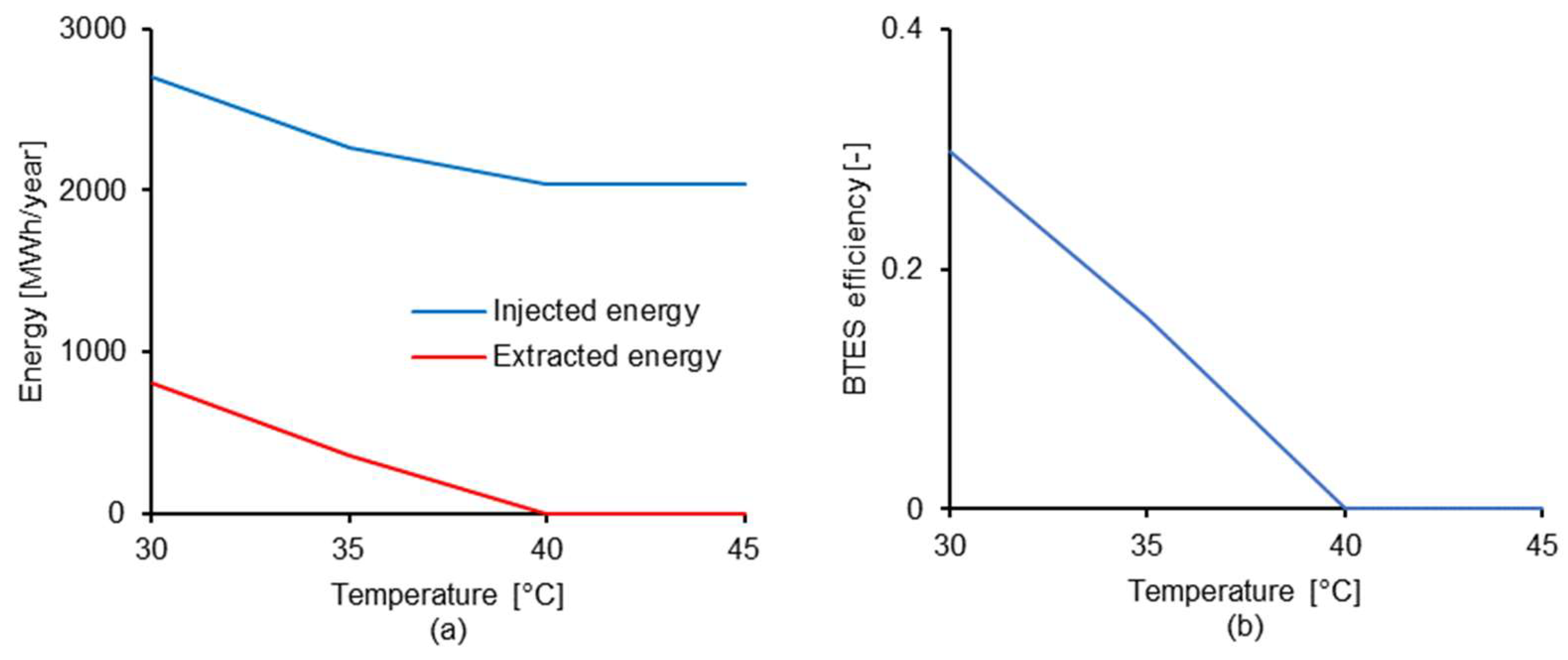
4.2.4. Useful Storage Temperature

Another key parameter for the performance of a BTES is the storage temperatures that are considered useful. In Figure 18, the effect on annual injected and extracted energy and BTES efficiency from minimum useful storage temperature is shown for the actual storage design and storage supply flow at heat injection, Case 6. When the useful storage temperature is reduced to 35 and 30 °C, it is predicted that 360 MWh/year and 800 MWh/year can be extracted respectively. In the latter case, this means a BTES efficiency of around 30%. In both cases, it was noted that minimum useful ground temperatures are reached before the end of the building heating season and that the temperature 10 m from the storage border, given by GT3, peaks at 25 °C during the year. This means that all the energy at the given heat extraction rate above 30 °C, until the date for which minimum ground temperatures are reached, can be extracted and that most of the energy above this temperature is present within the borehole field. The latter is also suggested by the almost linear relationship seen for extracted energy between 30 and 40 °C. Other operational conditions can be created by using a heat pump for the extraction of heat, in which case it is possible to make use of stored energy down to the natural ground temperature as well as continuing heat extraction in that state.

5. Conclusions

In this study, the large-scale industrial BTES at Xylem, Emmaboda was modelled in the IDA ICE 4.8 environment using the GHX module and compared to three years of measured storage performance. To describe the combined conductive and convective heat transfer in the ground, an effective ground thermal conductivity was used, which was determined from measured storage data. The model was then used to investigate the performance of the storage by changing such parameters as storage supply flow characteristics at heat injection, borehole spacing and borehole depth.

The three-year comparison between the modelled and measured storage performance shows that the performance of large-scale BTES with intermittent heat injection and extraction can be predicted with high accuracy. These predictions differed little when the simulation time step was varied from one hour up to four weeks regarding periods of heat injection only. However, a small time step was necessary to accurately predict the periods including the intermittent heat injection and extraction.

From the parametric study, the following conclusions can be drawn:

• For the investigated storage supply flows at heat injection, 10–20 l/s and 40–80 °C, a high temperature in the supply flow was more important than a high flow rate in order to achieve high annual heat extractions
• For a BTES there is a borehole spacing and depth at which heat extraction is the highest, which are possible to determine with the use of a numerical model such as the one used in this study
• Annual heat extraction quickly reduced as the spacing was decreased from the spacing yielding the highest annual heat extraction, whereas the reduction in annual heat extraction was quite slow when the spacing was increased from this point.
• Annual extracted energy was barely affected by a change in the effective ground thermal conductivity. However, the impact of the effective ground thermal conductivity is likely to have been greater at a higher temperature difference between the storage supply flow and the minimum storage temperature considered useful.
• Annual energy that could be extracted from the storage increased almost linearly with a decrease in the minimum storage temperature considered useful when the latter was decreased from 40 to 30 °C.

References

1. Rad, F.M.; Fung, A.S. Solar community heating and cooling system with borehole thermal energy storage -review of systems. Renew. Sustain. Energy Rev. 2016, 60, 1550–1561. [Google Scholar] [CrossRef]
2. Başer, T.; Lu, N.; McCartney, J.S. Operational response of a soil-borehole thermal energy storage system. ASCE J. Geotech. Geoenviron. Eng. 2015, 142, 04015097. [Google Scholar] [CrossRef]
3. Gao, L.; Zhao, J.; Tang, Z. A review on borehole seasonal solar thermal energy storage. Energy Procedia 2015, 70, 209–218. [Google Scholar] [CrossRef]
4. Pavlov, G.K.; Olesen, B.W. Seasonal solar thermal energy storage through ground heat exchangers-Review of systems and applications. In Proceedings of the 6th Dubrovnik Conference on Sustainable Development of Energy, Water and Environment Systems, Dubrovnik, Croatia, 24–28 September 2011. [Google Scholar]
5. Başer, T.; McCartney, J.S. Transient evaluation of a soil-borehole thermal energy storage system. Renew. Energy 2018. [Google Scholar] [CrossRef]
6. Choi, J.C.; Lee, S.R.; Lee, D.S. Numerical simulation of vertical ground heat exchangers: Intermittent operation in unsaturated soil conditions. Comput. Geotech. 2011, 38, 949–958. [Google Scholar] [CrossRef]
7. Nordell, B.; Hellström, G. High temperature solar heated seasonal storage system for low temperature heating of buildings. Sol. Energy 2000, 69, 511–523. [Google Scholar] [CrossRef]
8. Gehlin, S.; Andersson, O. Geothermal Energy Use, Country Update for Sweden. In Proceedings of the European Geothermal Congress 2016, Strasbourg, France, 19–23 September 2016. [Google Scholar]
9. Lundh, M.; Dalenbäck, J.-O. Swedish solar heated residential area with seasonal storage in rock: Initial evaluation. Renew. Energy 2008, 33, 703–711. [Google Scholar] [CrossRef]
10. Bauer, D.; Marx, R.; Nußbicker-Lux, J.; Ochs, F.; Heidemann, W.; Müller-Steinhagen, H. German central solar heating plants with seasonal heat storage. Sol. Energy 2010, 84, 612–623. [Google Scholar] [CrossRef]
11. Sibbitt, B.; McClenahan, D.; Djebbar, R.; Thornton, J.; Wong, B.; Carriere, J.; Kokko, J. The performance of a high solar fraction seasonal storage district heating system-five years of operation. Energy Procedia 2012, 30, 856–865. [Google Scholar] [CrossRef]
12. Giordano, N.; Comina, C.; Mandrone, G.; Cagni, A. Borehole thermal energy storage (btes). First results from the injection phase of a living lab in torino (nw italy). Renew. Energy 2016, 86, 993–1008. [Google Scholar] [CrossRef]
13. Lhendup, T.; Aye, L.; Fuller, R.J. Thermal charging of boreholes. Renew. Energy 2014, 67, 165–172. [Google Scholar] [CrossRef]
14. Lanini, S.; Delaleux, F.; Py, X.; Olives, R.; Nguyen, D. Improvement of borehole thermal energy storage design based on experimental and modelling results. Energy Build. 2014, 77, 393–400. [Google Scholar] [CrossRef] [Green Version]
15. Catolico, N.; Ge, S.; McCartney, J.S. Numerical modeling of a soil-borehole thermal energy storage system. Vadose Zone J. 2016, 15. [Google Scholar] [CrossRef]
16. Giordano, N.; Kanzari, I.; Miranda, M.M.; Dezayes, C.; Raymond, J. Underground Thermal Energy Storage in Subarctic Climates: A Feasibility Study Conducted in Kuujjuaq (QC, Canada). In Proceedings of the International Ground Source Heat Pump Association, Stockholm, Sweden, 18–19 September 2018. [Google Scholar]
17. Xu, L.; Torrens, I.; Guo, F.; Yang, X.; Hensen, J.L.M. Application of large underground seasonal thermal energy storage in district heating system: A model-based energy performance assessment of a pilot system in chifeng, china. Appl. Therm. Eng. 2018, 137, 319–328. [Google Scholar] [CrossRef]
18. Cui, P.; Diao, N.; Gao, C.; Fang, Z. Thermal investigation of in-series vertical ground heat exchangers for industrial waste heat storage. Geothermics 2015, 57, 205–212. [Google Scholar] [CrossRef]
19. Long-Term Performance Measurement of Gshp Systems Serving Commercial, Institutional and Multi-Family Buildings. Available online: https://heatpumpingtechnologies.org/annex52/wp-content/uploads/sites/60/2017/11/legaltextieahptannex52v1320171023.pdf (accessed on 10 January 2019).
20. Nilsson, E.; Rohdin, P. Performance evaluation of an industrial borehole thermal energy storage (btes) project-Experiences from the first seven years of operation. Renew. Energy 2019, 143, 1022–1034. [Google Scholar] [CrossRef]
21. Nordell, B.; Liuzzo Scorpo, A.; Andersson, O.; Rydell, L.; Carlsson, B. The HT BTES Plant in Emmaboda; Division of Architecture and Water, Luleå Unversity of Technology: Luleå, Sweden, 2016. [Google Scholar]
22. Bring, A.; Sahlin, P.; Vuolle, M. Models for Building Indoor Climate and Energy Simulation; Department of Building Sciences, KTH Royal Institute of Technology: Stockholm, Sweden, 1999. [Google Scholar]
23. Achermann, M. Validation of Ida Ice, version 2.11.06; Hochschule Luzern: Luzern, Sweden, 2000. [Google Scholar]
24. Description of the Ida Ice Borehole Model. EQUA Simulation AB. Available online: www.equa.se (accessed on 1 September 2018).
25. Fadejev, J.; Kurnitski, J. Geothermal energy piles and boreholes design with heat pump in a whole building simulation software. Energy Build. 2015, 106, 23–34. [Google Scholar] [CrossRef]
26. Li, M.; Lai, A.C.K. Review of analytical models for heat transfer by vertical ground heat exchangers (ghes): A perspective of time and space scales. Appl. Energy 2015, 151, 178–191. [Google Scholar] [CrossRef]
27. Patricia, M. Modelling and Monitoring Thermal Response of the Ground in Borehole Fields. Ph.D. Thesis, KTH Royal Institute of Technology, Stockholm, Sweden, 2018. [Google Scholar]
28. Incropera, F.P.; Dewitt, D.P.; Bergman, T.L.; Lavine, A.S. Fundamentals of Heat and Mass Transfer, 6th ed.; John Wiley & Sons Inc.: Hoboken, NJ, USA, 2006. [Google Scholar]
29. Eppelbaum, L.; Kutasov, I.; Pilchin, A. Applied Geothermics; Springer: Berlin/Heidelberg, Germany, 2014. [Google Scholar]
30. Welsch, B.; Rühaak, W.; Schulte, D.O.; Bär, K.; Sass, I. Characteristics of medium deep borehole thermal energy storage. Intern. J. Energy Res. 2016, 40, 1855–1868. [Google Scholar] [CrossRef]
Figure 1. Heat distribution network at Xylem, Emmaboda.
Energies 12 02263 g001
Figure 2. Layout of the borehole thermal energy storage (BTES) at Xylem, Emmaboda. The BTES consists of 140 boreholes, divided into seven sections, A–G, of 20 boreholes each. GT1–4 are temperature sensors inserted into the ground for storage operation and monitoring.
Energies 12 02263 g002
Figure 3. Schematic of the borehole heat exchanger. The open borehole heat exchanger design means that the heat carrier, being a mixture of groundwater and externally added water, has direct contact with the borehole wall.
Energies 12 02263 g003
Figure 4. Illustration of the intermittent heat injection and extraction present at Xylem, Emmaboda, shown by the storage supply and return flow temperature (a) and mass flow rate (b).
Energies 12 02263 g004
Figure 5. Measured storage supply flow temperature (a) and mass flow rate (b) at weekly average values.
Energies 12 02263 g005
Figure 6. Model layout, consisting of the IDA ICE GHX component, borehole inlets and outlets, input files for supply flow and outdoor air temperature, and logical and mathematical operators for storage operation and energy calculations.
Energies 12 02263 g006
Figure 7. Illustration of the criteria for storage annual steady state: (a) ground temperatures and (b) injected energy. In this case, annual steady state is considered to have been reached in year six.
Energies 12 02263 g007
Figure 8. Injected (a) and extracted (b) energy, calculated versus measured. The relative difference between measured and calculated data is associated with right y-axis.
Energies 12 02263 g008
Figure 9. Ground temperatures, calculated versus measured: (a) GT1, (b) GT2, (c) GT3, and (d) GT4. The relative difference between measured and calculated data is associated with right y-axis.
Energies 12 02263 g009
Figure 10. Calculated injected (a) and extracted (b) energy for different time steps.
Energies 12 02263 g010
Figure 11. Calculated ground temperatures, (a) GT1, (b) GT2, (c) GT3 and (d) GT4, for different time steps.
Energies 12 02263 g011
Figure 12. Annual injected (a) and extracted (b) energy as a function of borehole spacing. Values given in legend parentheses are the mass flow rate and temperature of the supply flow at heat injection respectively. 4 m is the actual borehole spacing.
Energies 12 02263 g012
Figure 13. Horizontal temperature distribution at half the borehole depth for when the temperatures within the borehole field at the considered line are at their annual minimum and maximum respectively. x is the distance from the borehole field centre and X is the distance between the borehole field centre and its border. The black line indicates minimum useful temperature.
Energies 12 02263 g013
Figure 14. BTES efficiency as a function of borehole spacing. Values given in legend parentheses are the mass flow rate and temperature of the supply flow at heat injection respectively. The actual borehole spacing is 4 m.
Energies 12 02263 g014
Figure 15. Annual injected energy (a), extracted energy (b) and BTES efficiency (c) as a function of borehole depth. Values given in legend parentheses are the mass flow rate and temperature of the supply flow at heat injection respectively. 144 m is the actual borehole depth.
Energies 12 02263 g015
Figure 16. Annual injected and extracted energy (a) and BTES efficiency (b) as a function of ground thermal conductivity for the actual storage supply flow at heat injection, Case 6.
Energies 12 02263 g016
Figure 17. Ground temperatures as a function of ground thermal conductivity for the actual storage supply flow at heat injection, Case 6. September 15 and May 15 are the start and end of the building heating season respectively.
Energies 12 02263 g017
Figure 18. Annual injected and extracted energy (a) and BTES efficiency (b) vs. minimum useful storage temperature for the actual storage supply flow at heat injection, Case 6.
Energies 12 02263 g018