1. Introduction
Power flow in distribution networks has traditionally been one-way towards the consumers from the substation. Now the scenario is changing, and networks are becoming bidirectional. This is due to substantial demand responses programs and interconnection of time-varying distributed generation (DG) at the distribution network (DN) level (medium voltage (MV) and low voltage (LV)) [
1]. Such active power system networks can be controlled properly only when the actual system state is known. In addition, there is a threat to network operators from bidirectional power flow causing operational issues for network security and voltage balance [
2], which forces network operators to carry out security assessment. For this objective, network states (voltage magnitudes (V) and angles (θ) at each bus), should be evaluated under all operating conditions [
3]. Based on the predicted network states, the other network parameters can be calculated, and the operators can run control modules and handle further operation effectively. To ensure the availability of estimated states, power industries today use observability analysis. However, the accuracy of the estimated states cannot be guaranteed due to a lack of sufficient real measurements and error in load/generation forecasting, especially in distribution grids. Topology change and flaws in data communication are some of the culprits for measurement inadequacy. The consequence of this is network un-observability, but the observability of this unobserved network can be reinstated by using some defined measurements [
4].
Any network can be classified as observable if it is possible to calculate all system states for the given measurements and topology. There are two predominant approaches for observability analysis: (a) topological: based on the graph theory analysis and decoupled measurement model and (b) numerical: based on the numerical factorization of gain matrices using either coupled or decoupled measurement models [
5]. In addition to these two methods, some other alternative approaches have also been applied for network observability assessment in power distribution grids. For instance, by defining the probability index, local observability assessment using graph theory criteria etc. [
6]. The method of distribution grid observability enhancement using a smart meter data is explained in [
7]. This method uses both time-varying injections and stationary conventional load data from the smart meter as metered and non-metered data for observability improvement. State estimation in this case is executed using the metered data from a small number of buses to solve the non-linear power flow equations over consecutive time instants. Observability of the network depends on number, type and locations of the measurements used, but not on the method followed. Generally, there are sufficient measurements available in the transmission network that these methods work well there. However, due to economic reasons, there are fewer measuring devices (e.g., power, current and voltage measurements) in distribution systems, especially at the MV level, so they are generally operated with reduced observability. On the other hand, in the emerging scenario, the use of smart meters at the LV level (every customer connection point) is rapidly increasing because of the availability of modern advanced metering infrastructures (AMI) [
1]. Some of the examples of increasing measurements at the distribution level are: (a) the European Union’s (EU) initiative to replace 80% of traditional electricity meters with smart meters by 2020 [
4], (b) installation of more than 70 million (nearly half of U.S. electricity customers) AMI in the United States (U.S.) [
8], etc. Therefore, in future there will be a huge amount of data available from almost every node in the LV distribution grid, and they will be stored in data centers such as data hubs. These data can be used for any applications. For control applications, these large amounts of data gathered by smart meters have to be processed and used in an economical way. Hence, smart selection of minimum key data from the huge pool of available data from customer locations as well as from other specific locations will enhance the observability of active distribution networks (ADNs), while at the same time, ensuring higher accuracy of the estimated states of the observable network is the main challenge [
7]. The Fisher information-based meter placement technique by minimizing errors in estimated state vector is proposed in [
9]. It uses the D-optimality criterion, and a Boolean-convex model is used for optimization of the problem formulation. A meter placement algorithm to improve the estimated voltage and angle at each bus in the network is described in [
10]. This technique is based on the consecutive upgrading of a bivariate probability index that is applied in medium voltage networks. The minimum meter placement technique discussed in this paper is a simple algebraic technique that can be applied in both MV and LV control applications. For MV grids, it will determine the best minimum metering locations, and for LV grids, it will identify the minimum key data from the huge pool of smart meter data. Using these smartly selected data, the respective networks can be fully observed with an accurately estimated network state from all nodes.
A reduced observability scenario below the substation is one of the reasons for the limited use of distribution state estimation (DSSE) by the utility. However, now, to address the challenges resulting from the increasing penetration of flexible resources and DGs at DN, real-time network models based on DSSE are becoming more essential for operation and control of the DN [
11]. In the available literature, many vital issues in the development of DSSE have been discussed [
12,
13,
14]. Proposed algorithms have been categorized based on simplification in order to speed up the estimation, selection of the state variables, and the procedures for integrating diverse measurements. Considering the choice of state variables, branch current-based and node voltage-based state estimators are the two main categories that would ultimately results in similar accuracy at the end [
15]. The WLS (weighted least square) method’s performance analysis with respect to the choice of state variables and comparisons on the basis of accuracy, performance and bad data detection capability were reported in [
16]. To use the estimated network state information for operation and control, state estimation has to be dynamic, irrespective of the method used for estimation. Dynamic state estimation is a recurrent estimation in a time sequence based on several measurement snapshots. For the estimation of large distribution networks, the execution time will be longer if we assume a single estimation process for the whole network. Therefore, distributed DSSE methods can be used to overcome such issues, executing the DSSE module in different sub-areas of the distribution network locally. Network division for this purpose can be carried out according to topological framework, geographical standpoint or measurement locations to solve the problem via local estimators in that particular sub-area. However, it is challenging to use DSSE in real life networks due to the limited number of real measurements, delay in communication, and un-synchronized measurements, which are detrimental to multi-area estimation accuracy [
15]. The Distribution System State Estimation procedure with multi area architecture is discussed in [
17]. It is based on a two-step procedure, i.e., local estimation followed by global estimation by using integrated measurement information from adjacent areas. The WLS estimation principle is used to identify the impact on the estimation accuracy of sharing the measurements among different areas. To monitor the dynamic behavior of the power system, for example, in order to know the quasi real-time operating condition in case of any fast-evolving contingencies, phasor measurement unit (PMU) measurements are included in the measurement set used by the state estimation [
18]. PMU measurements comprise a voltage phasor at a bus and a current phasor through the line incident to that bus, and have sampling synchronized to a common reference through a GPS signal at widely spread locations [
19]. A number of approaches can be found in the literature to include PMU data set into the existing conventional measurement setup [
20]. If only voltage and current measurements from PMU are used, the state estimation problem will be linear, but it will be nonlinear with the presence of both PMU and conventional measurements. Therefore, to linearize the problem, the measured phasors in polar form can be converted to an equivalent rectangular form. Key challenges due to the inclusion of PMU measurements include: false data injection attack in the wide area measurement system [
21], convergence problem of the hybrid state estimator during the iterative process due to uncertainty introduced by the instrument transformers, their connection with digital equipment and A/D converters [
22], etc. On the other hand, to overcome the limitation of real measurements, when large number of virtual measurements (that may have significant uncertainties) are used to make the network observable, there is a high possibility of system states deviating from their actual values. Hence, the optimal number and specific type of real measurements collected from specific locations are essential to address the necessities of applications for real-time operation with high accuracy [
23,
24]. Therefore, the challenges to develop new real-time monitoring and management solutions for smart grid still exists, such as:
Accurately observing the whole distribution network using minimum real data and maximum pseudo measurements.
Developing an integrated approach for accurate, adaptive and efficient DSSE methodologies equipped with minimum measurement technique for wide area monitoring that can be implemented in the active distribution network.
Identifying the practical trade-off between network observability, number of installed measuring devices, and accuracy of estimated states.
These challenges related to measurement data utilization and its trade-off in DMS to enhance the state estimation are addressed in this paper. The main contributions of the paper are: development of a unified network observability assessment technique using minimum measured data, development of a technique to identify critical measuring locations for SE based on a bus prioritization approach, and formulation of a procedure to evaluate the trade-off between SE accuracy and the number of real measurement devices to be considered. This enables the user to maintain estimation precision in the distribution network with a lower burden. Overall, the paper is structured as follows: the problem statement is described in
Section 2 and the overall methodology and algorithm is explained in
Section 3, which covers observability assessment, meter placement analysis, network parameter estimation and accuracy trade-off analysis between the number of used measurements and the accuracy of estimated states. Improved forecasting for pseudo measurements of loads/generations are stated in
Section 4. Case studies with results and discussion are presented in
Section 5. The conclusions of the paper and the directions of future work are finally summarized in
Section 6.
2. Problem Statement
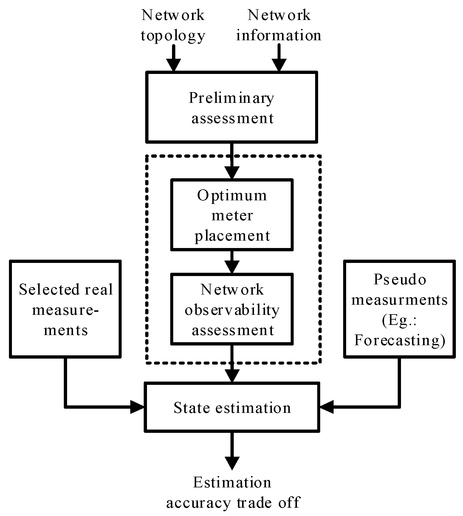
Network topology, grid parameters, field measurements and system data correlation are never fixed; everything depends on the operating conditions. Due to these uncertainties, network modelling is never perfect, and inaccuracies are contained in the DSSE results. When the database is extremely large, network reduction may help to improve the estimation accuracy to some extent. Key essential tasks for the enhancement of observability and improvement of accuracy of online models are: synergize the massive diverse data in different data formats from several information systems, synchronize the polling cycles, and minimize the communication delay and variation in measurements [
25]. Generally, three types of measurements are considered in DSSE [
15].
Equipment connectivity status received from Geographic Information System (GIS).
Real-time measurements from distribution SCADA systems (e.g., voltage, current and power flow) embedded with measuring units (e.g., smart meters, PMU, remote terminal unit (RTU), AMI, etc.).
Customer/prosumer’s demand and DER output data (active and reactive power) from data management system.
If all of these numerous measurements are used, it may give better accuracy, but will require additional bandwidth for a communication infrastructure with suitable reliability. This will then lead to other problems, like data overload and extra financial burden. On the other hand, limited use of real-time measurement cannot ensure the overall observability of the network [
26,
27]. To minimize the use of real measurements, a large number of pseudo and virtual measurements can be used. Load and generation forecasts are pseudo measurements, whereas zero voltage drops in closed switching devices, zero bus injections at the switching station nodes, etc., are virtual measurements. However, changes in the behavior of power consumption because of external factors like new tariff structures, environmental condition, etc., and the allocation of greater weight to virtual measurements and lower weight to pseudo measurements may lead to ill-conditioned systems [
15]. Therefore, this problem is tackled in this paper by utilizing maximum pseudo measurements only (injection measurements calculated from forecasted load/generation profiles) with a trade-off analysis where DSOs can achieve observability in their distribution grids with higher accuracy in estimated states by using minimal real measurements. The overall workflow for this problem is presented in
Figure 1. As shown in
Figure 1, for the particular network parameter to be estimated (in this work voltage in each bus), the type and combination of measurements (PV or PQ or IV or PQI, etc.) required are identified based on a preliminary assessment based on the available network topology and information. The best combination of measurements for real networks is identified in this preliminary assessment using the method explained in [
28], and consists of analyzing the impact of number and placement of smart meter data on errors in state estimation using a standard network. This is a onetime exercise, and there is no need for repeated analysis of the preceding calculations. This is the first step, and this will identify the key measurement parameters and their locations, to a certain extent. It is followed by the observability assessment of the network with minimum meter placement, which is described in
Section 3, below. Once the network is identified as being observable with minimum measurements, the state estimation (SE) is triggered. For the SE, real data from the identified key meters, together with the pseudo measurements for the rest of the nodes (which have no real measurements available), are supplied. Finally, a trade-off analysis between the number of real measurements used, the level of network observability and state estimation accuracy is carried out. For the estimation of network parameters, the weighted least square-based approach based on the Newton-Raphson method is applied. A detailed explanation of the methodology followed for each working block represented in
Figure 1 is explained in
Section 3 and
Section 4 below.
3. Observability Assessment
The first stage in the assessment of observability is to choose estimation variables, and the best combination of parameters to be measured. This is termed preliminary assessment in this paper. It will minimize the iteration cycle in SE and give the minimum estimation error to a certain extent. For voltage estimation, line flow measurements are found to be more crucial [
28]. It depends on network type and the variables to be estimated. As described in [
28], if the parameters to be measured from specific locations are selected properly, better estimation quality can be achieved even with fewer real measurements. As explained above, once the estimation variables and the proper combination of measurements of parameters are selected, the actual network observability assessment will start, followed by state estimation. If the network is identified as being unobservable, all branches in it that cannot be observed have to be determined first. Then, by removing unobservable branches, the network can be divided into many individual observable islands that can be treated individually and merged later to have a single observable island. To improve the overall observability of the whole network, further analysis on the determination of specific measurement locations and the selection of minimum measurements has to be carried out [
29]. The proposed integrated algorithm for observability assessment and its application in SE is given in
Section 3.
Algorithm for Network Observability, SE and Accuracy Trade-Off
Algorithm for Observability Check (AOC):
Step 1: Calculate measurement Jacobian matrix (H) and its gain matrix (G) [
5,
29].
Step 2: Perform triangular factorization of G and evaluate its triangular factors (L: lower factor). Using triangular factors, identify diagonal matrix (D) [
5].
Step 3: Test for zero pivot in D, and if D is equal to one, network is observable [
29]. If network is observable proceed to state estimation for this go to ‘step one in Algorithm for SE formulation’; otherwise go to step four.
Step 4: Determine test matrix W using equation: and calculate another test matrix C using equation: where A is incidence matrix of branches and buses.
Step 5: Identify unobservable branches corresponding to the row in ‘C’ with at least one non-zero element. Remove all unobservable branches
Step 6: Prepare the list for probable measurement points. Prioritize them. Highest priority for placing a meter is assigned to the bus that has the maximum number of incident lines in the unobservable region. Line flow measurement from the branches between the observable islands and the injection measurements from the buses at the boundary of these islands are the next most suitable candidate measurements, which can merge the islands. Current flow measurement at the beginning of the feeders are another prioritized measurement, and feeders with greater length and higher number of branches are of higher priority among the others. Select the measurement points based on priority, and go to step one for all new measurements added.
Normally in MV distribution systems, there is a limitation due to economic concerns on the availability of adequate real measurements from each node; therefore, a large number of pseudo measurements are used for the analysis. Therefore, even though the network is identified as being observable, there is a high chance that an estimated state can differ significantly from the actual state. Hence, re-examination of network observability considering the accuracy of the estimated states is recommended.
State Estimation Formulation:
SE is the core of the security analysis function in power systems. It acts like a filter between raw measurements and application functions like control and protection modules. Based on the available measurement sets, it estimates the network status. The state of the network is defined by voltage magnitude
and angle
at every bus (i.e., 2n state variables) for an ‘n’-bus power system network [
5,
30]. The basic algorithmic steps for network state estimation are given below:
Step 1: Represent the network model by state vector as shown in Equation (1). If bus 1 is considered to be the reference, it is set as (
).
The measurement vector (z) is related to the state vector (x) by a nonlinear function (h) and a vector of measurement error (e) as given in (2). These functions and their behavior are dependent on network topology and actual power flow.
Step 2: Define the objective function as represented in Equation (3) and minimize it for the network estimation. To minimize this objective function, WLS—the most commonly used method—is used in this paper. Here, R,
and m represent the measurement error covariance matrix, measurement variance and the number of measurements, respectively.
This approach determines the variance of the estimated state variables by:
Where the diagonal elements of cov(x) represent the variance of the estimated state variables.
Step 3: Once the all the network states are estimated, accuracy is evaluated based on the number of measurements used. Go to ‘step one of algorithm for accuracy trade-off in state estimation’.
Algorithm for accuracy trade-off in state estimation (AAT):
Step 1: Choose the desired confidence level (CL). This represents the risk that the true value goes beyond the boundary of the confidence interval (CI), i.e., the lower the CL, the higher the risk, and vice versa [
31].
Step 2: Calculate the probability density function (PDF) of the estimated states using Equation (7) [
5].
Where I is the total number of network parameters that has to be estimated, and for each network parameter ‘i’, its estimated value is
for i = [1, 2, ..., i, ..., I].
represents the variance of ‘i’, whereas
denotes a possible value of this parameter ‘i’. There are many methods for calculating the PDF of an estimated parameter in order to calculate CI. Gain matrix-based approaches assuming Gaussian distribution have been used in this work, since the formulated observability assessment method is independent of the PDF calculation method [
31,
32].
Step 3: Calculate confidence interval (CI) for each defined PDF. For predefined values of CL, the CI end points,
and
, of the estimated parameter i have to satisfy Equations (8) and (9) [
31].
The CI can be calculated by multiplying the standard deviation by the coverage factor related to the predefined CL.
and
are the endpoints of the CI and represent the accuracy of the estimated value of parameter i. Then, calculate the maximum expected difference between
and its true value as given by Equation (10).
Step 4: Access the estimation accuracy. If Equation (10) is satisfied, the estimation can be classified as accurate and stop the process. Otherwise, go to step five.
Step5: Redefine the measurement placement with next possible measuring option, change the ratio of real and pseudo measurements, and go to ‘step six of algorithm for observability check’.
The overall methodology discussed in
Section 3 in the form of different algorithms can be combined to form a compact flowchart as shown in
Figure 2, systematically interlinking all the mathematical models (Equations (1)–(10)) for the complete analysis.
5. Case Study
The methodology described in
Section 3 and
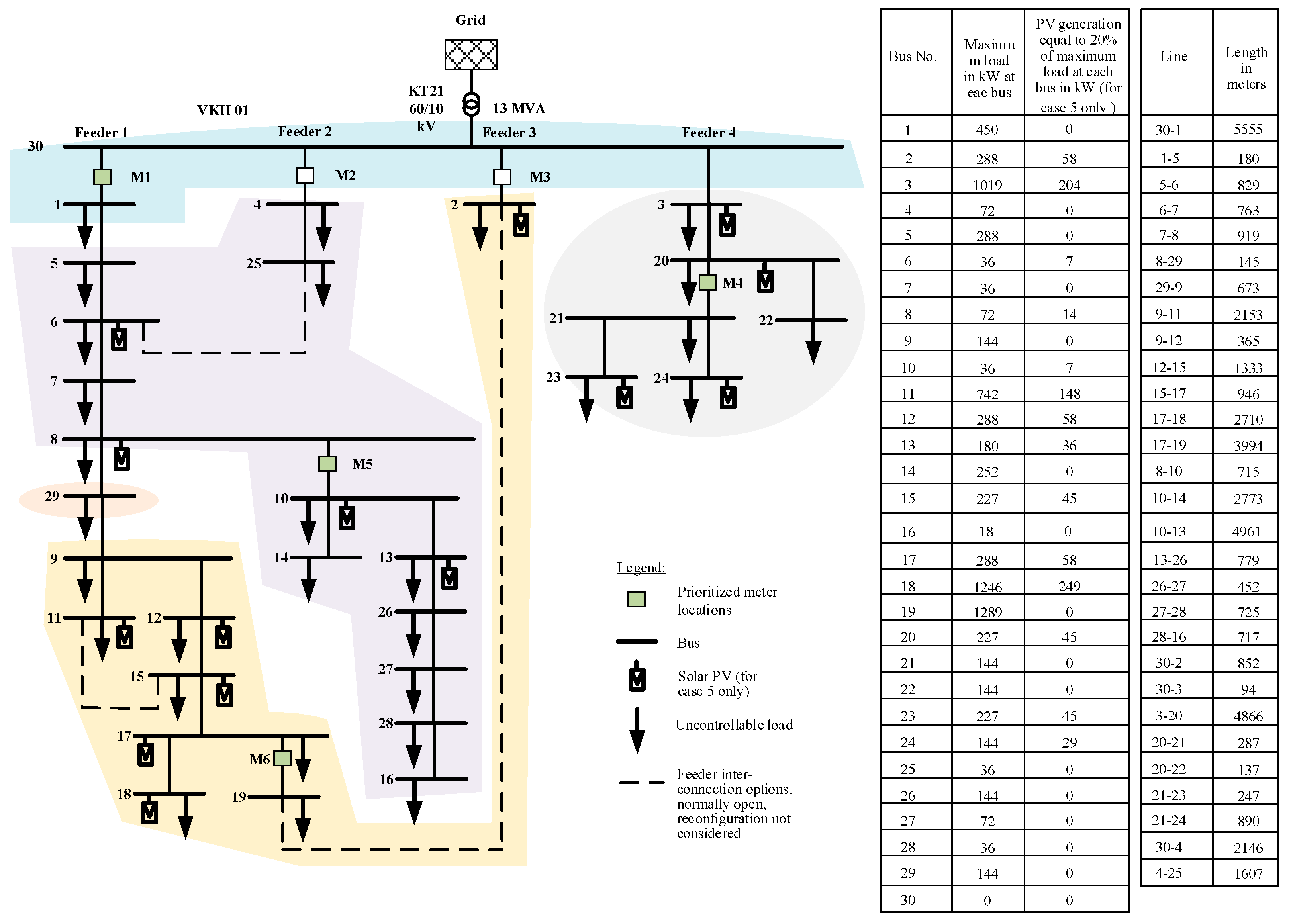
Section 4 is simulated for a real network and is discussed in the following sections. To demonstrate the applicability of the proposed methods, case studies have been performed on a model of a 52-bus MV distribution network from the Lind area in Denmark. For simplicity, the actual network is reduced to a 30-bus network preserving its radial nature and feeder connections, as given in
Figure 3. While reducing the network, 24-load points are lumped up, i.e., five loads to bus3, three loads to bus 11, one load to bus 12, three loads to bus 13, two loads to bus 14, one load to bus 17, four loads to bus 18, and five loads to bus 19. Therefore, with this setup, in the test network, the maximum load of 1289 kW is at bus 19 and next largest load size (1246 kW) is at bus 18, while the minimum load of 18 kW is at bus 16. The typical R/X ratio of distribution lines in this network varies between 7.07 to 1.38.
The types of load and the state of the transformer tap changer will have an impact on network performance. For simplicity, an operating scenario in which all distribution transformers (buses 1 to 29) are loaded with a capacity factor of 40% and load power factor of 0.9 is assumed for the load flow and network measurements. The load distributions in all of the buses in this scenario are given in the table included in
Figure 3. This operating condition is the peak load scenario for the main transformer (KT21). Another assumption is the presence of solar PV, which is considered to be available only in case 5.
Initially (case 1), it is assumed that 14 measurements from the substation (bus 30), the far end of the feeders (buses: 2, 11, 14, 16, 18, 19, 22, 23, 24, 25), and lines (6–7, and 17–19, i.e., close to the substation and at the far end of the longest feeder) are available. Thus, measurements are available for eleven power injections (net active/reactive power at the bus that can be obtained via load generation forecasting), two line flows (active/reactive power), and one voltage (at the substation). As per this measurement configuration, the network observability is analyzed by determining the gain matrix and its triangular factors. The upper triangular factor of the measurement gain matrix is evaluated and its diagonal elements (D) are identified. It is found that 28 elements out of 30 in D are zero. This shows the network is unobservable, and it is then divided into ten observable islands by removing the unobservable branches, as shown in
Table 1. The candidate measurements list is prepared in consideration of the boundary of observable islands. To justify the requirement of bus prioritization, initially, power injection measurements close to buses 3, 6, 12, 4, 27, and 29 are selected arbitrarily from the list as case 2. After each added measurement, observability assessment is carried out. The upper triangular matrix is updated and its new diagonal elements (D’) are found, in which 27 zero pivots are observed. Since significant improvement has not been achieved, the network is divided into eight observable islands. Now, the candidate measurements are prioritized according to the description given in step 6 of the observability algorithm in
Section 3. Only 10 measurement locations (5, 7, 8, 10, 15, 17, 20, 21, 25 and 30) out of 16 candidate sites are considered, and those remaining are filtered out. In reality, both power/current flow and power injection measurements can be measured from the same smart meter. Based on the user’s requirements, the smart meters can be tuned to measure specific parameters. This option is available in most of the smart meters available today. Therefore, for the new injection measurements to be added for case 3, locations 7 and 15 from the priority list, which are close to the branch flow measurements, are selected. Also, line 30–1, and 20–21 for the branch flow measurement are considered to be added as per priority for case 3. After these measurements have been added, the new upper triangular matrix is evaluated, and updated diagonal elements (D’’) are found. It is noticeable that observability is improved in this case due to significantly reduced number of zero pivots. However, the network is not fully observable. In this case, five observable islands are identified. Next, in case 4, the candidate list is updated based on the observable islands in this case, and prioritized as 5, 8, 10, 15, 20, 25, 29 and 30. Injection at locations 15 and 20 from the boundary of the islands that are observable are now selected, together with the branch flow in lines 30–1, 20–21, 8–10 and 17–19 (M1, M4, M5 and M6), as per priority. The diagonal elements of the upper triangular matrix (D’’’) from the updated triangular factors are calculated. In matrix D’’’, only one zero pivot can now be observed. This shows that the network is now fully observable. These case studies for network observability are summarized in
Table 1. Once the network observability has been assessed, network states are estimated for each case using selected real measurements and pseudo measurements (the forecasted load and generation value at each bus that will give net injection measurements at the respective buses). This is followed by accuracy trade-off evaluation. The case studies for state estimation and accuracy trade-off evaluation carried out after the network observability assessment are presented in the subsequent
Section 5.1 and
Section 5.2.
5.1. Parameter Estimation and Accuracy Trade Off
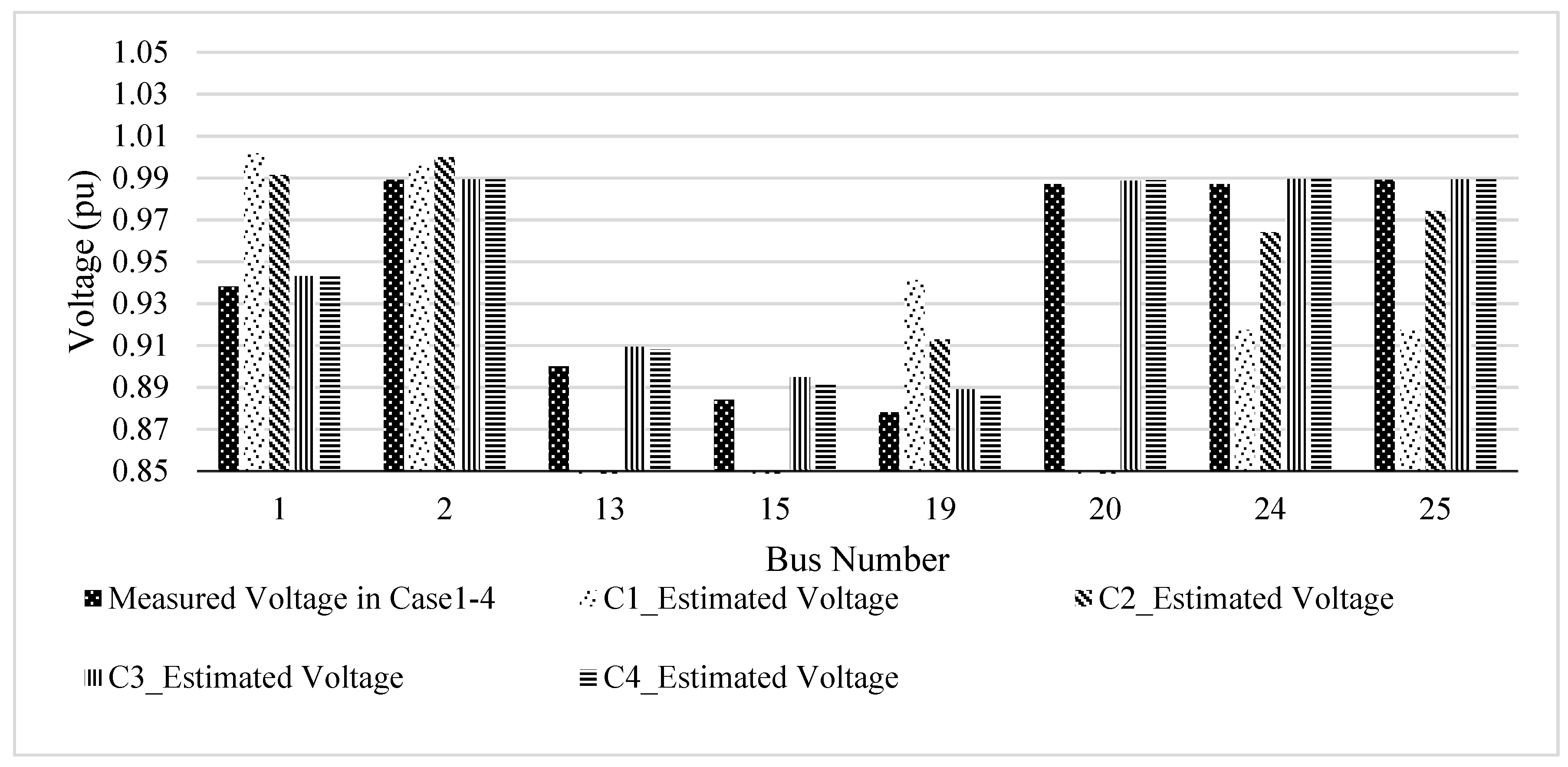
Network observability setups with the minimum number of identified measurements can only be useful if this configuration can be used to estimate network states close to the actual values. Therefore, for instance, voltage magnitude is estimated for each case and compared with actual measured values, as shown in
Figure 4 for selected buses close to the substation (buses 1 and 2), the far end (buses 19 and 24), and the middle (buses 13, 15, 20 and 25) of the feeders. In the measurement a minimum voltage of 0.88 pu is observed at bus 18 when all feeder interconnection options (6–25, 11–15 and 2–19) are open, i.e., at the end of the first radial (the longest radial feeder in the setup), which violates the grid code [
35]. Buses 13 and 15 are also in the same feeder as bus 18, but are towards the substation, so they have slightly more voltage than in bus 18. Since buses 25, 2, 20, and 24 are in the 2nd, 3rd and 4th feeders (short feeders, i.e., lightly loaded compared to the first feeder), respectively, they have higher bus voltages (close to 0.99 pu). In real network operation, reconfiguration is used to maintain the grid code (e.g., minimum voltage of 0.95 at bus 16 while closing 2–19 and opening 9–12), but reconfiguration is not considered in this paper. In addition, a fixed load of 40% is considered in this work to see the performance of the proposed algorithm in special cases (case 1–7). This loading scenario may not exist all the time in real network operation. The results are obtained from a series of repeated simulations in MATLAB (observability analysis) and DigSILENT power factory (load flow, measurement setup, and state estimation) and snapshots of the results are shown here. The accuracy class of all smart meters is considered to be 0.5, as per IEC 62053-11 [
36]. In this simulation, bus 30, which is close to the main substation, is considered to be the reference bus, the measured voltage of which is 0.99 pu. The first feeder is extremely long compared to the other three feeders, so lower voltages are observed in the buses (e.g., in buses 1, 13 15 and 18) in this feeder. Meanwhile, the other three feeders are short compared to the first feeder, so the voltages in the buses (e.g., in buses 2, 20, 24, 25) in these feeders are almost the same as the reference voltage, i.e., 0.99.
As expected, in case 1, where measurements are insufficient, the network is not fully observable, i.e., it is not possible to estimate the bus voltage for all buses (e.g., buses 13, 15 and 20), as is shown in
Figure 4, where the magnitude of the estimated voltage for these buses is not available. In this case, overall network observability, which is a prerequisite for SE, is established by reducing the number of control variables (suspending the states to be estimated for buses 13, 15 and 20), and the bus voltages for rest of the buses is estimated. In case 2, real measurements (30%) are supplied, but without any bus prioritization, resulting in there being no significant improvement in the network state estimation. However, after applying the bus prioritization technique, i.e., by selecting only key measurements from the selected buses (only 22% real measurements) as in case 3, significant improvement is achieved. All network states including bus 13 and 15 are estimated due to the key added measurements from the prioritized buses. In case 4, which has 4% more real measurement than in case 3, all network states are estimated, with estimated states being closer to the real values. This verifies the network observability assessment results presented in
Table 1. Comparison of parameter estimation errors in different case studies for the selected bus voltages are shown in
Figure 5. As seen here, it is a trade-off between higher accuracy and investment in measuring devices. The magnitude of error shows the deviation of estimated quantity from its respective measured value. Positive error means overestimation and negative error means underestimation. The magnitude of error depends upon the number, type and location of the measurements considered for the respective case studies. In case 3, a maximum error of 1.24% (in bus 19) using fewer real measurements can be achieved. Also, further improvement is observed with a maximum error of 0.96% in the estimated voltages in case 4.
5.2. Worst Case Scenario Analysis
Under any operating conditions, all possible states have to be estimated to confirm the observability of a network. Therefore, the algorithm is tested in worst case scenarios, in which network states are likely to be violated. These scenarios are generally used during the planning phase of grid network operation, so it is known to DSOs [
37,
38]. Following worst case scenario (a), which is one of the worst operating scenarios, in which more DGs are integrated in the distribution network, other scenarios (b), (c) and (d) that could happen in real network operation have been set up to test the applicability of the method:
Case 5 (C5): Minimum load and maximum generation. Minimum load (30% of maximum load at each bus) and maximum generation (20% of maximum load at each bus where generation is available) respectively.
Case 6 (C6): Parameter estimation when line flow measurements (M4, M5 and M6) have an error of plus 5% of nominal reading.
Case 7 (C7): Parameter estimation with large error on pseudo measurements models (over forecasting of load by 10%).
Network measurement setup is designated as a fully observable condition, i.e., as in case 4, which is then re-simulated to estimate the network parameters for the scenarios mentioned in cases 5–7; a snapshot of the results for voltage estimation is shown in
Figure 6 and
Figure 7.
As seen in
Figure 6, i.e., in case 5, it is found that using the same technique, network parameters can be estimated at close to their true value (maximum error 0.97%) even when the network is more active (i.e., in the presence of DG). About 0.01% more error than case 4 is noticed in case 5. This is because the estimator is modelled using net injection measurements at each bus, which logically include the impact of DG. However, a change in the system state due to RE penetration can result in the WLS estimator becoming trapped in local minima, and can add some error if the network is large, with the highest number of DGs [
6]. From
Figure 7, it can be seen that different patterns of impact are seen in case 6, i.e., only voltage estimates close to erroneous measurement points are more influenced (buses 13, 15, and 19). This is because the accuracy of the estimator is inversely proportional to the level of measurement error, and this will be reflected to the estimated states, which are close to the erroneous meter; furthermore, the effect could also be different with different types of measurements [
39]. However, negligible impact is seen in the other buses, which are further away from the erroneous meters. The level of impact depends on the closeness of the meter and the number and locations of available meters in the same feeder [
6,
39]. This is valid for a radial feeder setup, which is the predominant case in most power distribution networks. The impact of forecasting error (case 7) can be reflected in the estimation error to some extent. This is because most of the pseudo measurements (load and generation at each bus) will be noisy and result in erroneous injection measurements in all buses. Therefore, estimated voltage magnitude will be lower than the real value in some buses due to the application of overestimated forecasting. As shown in
Figure 7, since the error for the forecasted load is plus 10% and the estimating variable is the voltage, not the load, at each bus, the maximum error recorded on voltage estimation in this situation (case 7) is only 1.1%. The magnitude of error on the estimated parameter depends on the number of pseudomeasurements used by the estimator that have been selected from an incorrectly forecasted load/generation.
Key results are summarized in
Table 2, showing the advantage of the proposed methodology over the conventional method. This shows the possibility of achieving higher accuracy in estimated states with the minimum use of real measurements (26%). The maximum error in the estimated states without applying the proposed technique is improved to 0.91 % (without considering DG) and 0.92% (considering DG). Even by using only 22% real measurements, all network states can be estimated with a maximum error of 1.14%. This proposed technique is a simple algebraic technique that identifies the minimum number of meters to be installed for full network observability. Therefore, it will be more economical and reliable than more complex methods, such as the Fisher information-based meter placement technique described in [
9], which uses the pre-specified number of additional measurement units from the set of candidate units. The highest-quality result (minimum SE error) is obtained with 23% real measurements (20 real measuring units, with each unit consisting of 3 real measurements, i.e., with 60 real measurements out of 260 measurements (both real and pseudo)) in the test network. Even though in the latter case, about 23% real measurements are used, technique followed is comparatively more complex than the proposed method.


