Article

Optimal Power Flow of Integrated Renewable Energy System using a Thyristor Controlled SeriesCompensator and a Grey-Wolf Algorithm

1
Department of EEE, GMR Institute of Technology Rajam, Rajam, AP 532127, India
2
Department of EEE, JNTUA CE Pulivendula, Pulivendula, AP 516390, India
3
Department of EEE, JNTUK Kakinada, Kakinada, AP 533001, India
*
Author to whom correspondence should be addressed.
Energies 2019, 12(11), 2215; https://doi.org/10.3390/en12112215
Submission received: 16 April 2019 / Revised: 16 May 2019 / Accepted: 30 May 2019 / Published: 11 June 2019
(This article belongs to the Section F: Electrical Engineering)

Abstract

:
Inrecent electrical power networks a number of failures due to overloading of the transmission lines, stability problems, mismatch in supply and demand, narrow scope for expanding the transmission network and other issues like global warming, environmental conditions, etc. have been noticed. In this paper, a thyristor-controlled series compensator (TCSC) is placed at the optimum position by using two indices for enhancing the power flows as well as the voltage security and power quality of the integrated system. A fusedseverity index is proposed for the optimal positionalong with a grey wolf algorithm-based optimal tuning of the TCSC for reduction of real power losses, fuel cost with valve-point effect, carbon emissions, and voltage deviation in a modern electrical network. The voltage stability index to evaluate the power flow of the line and a novel line stability indexto assessthe line capacityare used. The TCSC is placed at the highest value of the fusedseverity index. In addition, an intermittent severity index (IMSI) is used to find the most severely affected line and is used for relocating the TCSC to a better location under different contingencies.Lognormal and Weibull probability density functions (PDFs)are utilized forassessing the output ofphotovoltaic (PV) and wind power. The proposed methodhas been implemented on the IEEE 57 bus system to validate the methodology, and the results of the integrated system with and without TCSC are comparedunder normal and contingency conditions.

1. Introduction

In the recent past interest in distributed generation has increased tremendously due to the cost of fuel, carbon footprint concerns, load demand, and its delivery ofclean power, etc. At present, the electrical power system is facing various problems like network communication, load demand, environmentalconstraints and limited expansion of lines that influencethe sustainability and reliability. These issues have encouragedresearchersto utilize solar and wind generation for the reduction of transmission losses, carbon emissions and fuel cost. These sources can be operated either in private or grid-connected modes.The idea of wind and solar associated with a conventional system, though innovative, has causedmore difficulties for planners and analysts due to the need toimprove voltage stability and sustainability. Researchers are searching for better strategies to utilize the maximum power with the current integrated energy systems. The optimization can achieve an optimum power solution within the predefined conditions. This developmentcan be possible by associating shunt and series devices and keeping voltageswithin specified limits. Lately, the improvement of power electronic devices providecontrol and isadaptable to FACTS. FACTS instruments can be utilized to control various parameters of the transmission lines in a powerful way. The capacity of these devices can be used appropriately by properly tuning and placement at a specific locationin the network and this leads to the reduction ofactive power losses and maintains stability. Various optimization methods have been proposed for obtaining the desired systemperformance.
In the literature, various distributedgeneration systems like wind, solar, etc. combined with conventional thermal generators are proposed to alleviate many of the concerns [1,2,3,4,5,6,7,8]. Abaci et al. [9] clarified the planning of generators considering the monetary criteria, valuesof shunt capacitors, load tap changers in the OPF outline. Shi et al. [10] have talked about and reviewed diverse systems utilized withOPF underwind power constraints and environmental cost benefits. Sichilalu et al. [11] have endeavored to consolidate a heat pump-based water heater model which is delivered by wind and a PV solar system considering price minimization and electricity tariff as an objective. Levron et al. [12] demonstrated control of stored energy to balance the power generation by renewable energy sources. Biswas et al. [13] have demonstrated some vulnerabilities of PV and wind, where the constraints are incorporated with conventional generators for the objective function. Reserve cost, penalty cost, and estimated cost of renewable energies areadditionally considered for taking care of the OPF issue.
HamzehAghdam et al. [14] demonstrated that line blackouts due to the failure of system components, overburden, and high infiltration of renewable energy sourcesmight influence the entire energy management of the system. Rao et al. [15] clarifiedthe optimum placement for SVC utilizing firefly and BAT algorithms. Hingorani et al. [16] explained and analyzed various devices for different types of electrical power system issues. Bali et al. [17] proposed a combined index-based optimal generation reallocation utilizinga harmony search algorithm. Kumar Gundavarapu et al. [18] recommended a disparity line-based utilization index for the ideal location of interline power flow controllers based on the resolutionof line flows using a firefly algorithm. Modarresi et al. [19] havedemonstratedvarious indices suitable for finding the frail lines and buses for optimal placement problems. Kim et al. [20] explained the available transfer capability for the power flow using the fuzzy sets. Nireekshana et al. [21] investigated the use of TCSC, SVC to enhance the power transfer capability using a cat swarm algorithm. Mansour et al. [22] proposed optimal placement for TCSC under the condition of voltage stability. Bhattacharyya et al. [23] demonstrated the optimal TCSC location aimed at the enhancement of power flow by setting the control parameters like generator outputs, tap changing transformers, etc.Over the last two decades, many metaheuristics algorithms have been developed. Some of them are utilized for the optimal power flow problems for various applications and objectives considering equality and inequality constraints. The novel algorithms used for optimum power flowinclude the krill herd procedure [24], particle swarm optimization (PSO) [25], adaptive group search optimization procedure [26] for multi-tasking functions. Mirjalili et al. [27] demonstrated a new meta-heuristic grey wolf algorithm in 2014 which provides thebest results as compared to existing optimizing methods.
This paper predominantly focuses on optimal power flow-based generation reallocation of a renewable integrated power system in the absence and presence of TCSC utilizing a grey wolf algorithm. A fused severity factorthat is a blend of a rapid voltage stability index (RVSI) and a novel line stability index (NLSI) has been framed to achieve the optimumposition of the TCSC device and isadditionally utilized to attain aprecise measurement of overburdened lines.RVSI is being used for the assessment of loaded linesconcerning line parameters and reactive power. NLSI is used for the estimation of the overloaded line concerning real power and resistance.FSI is determinedto find the frail lines connected to the buses of the power system. Every one of the lines is positioned in descending order based on the fused severity index. The line sets that have the maximum value of FSIareviewed asoptimum placement locations for TCSC. The multi-objective task consists of active power loss, carbon emission, voltage deviation and fuel cost with valve-point impact has been formulated for optimum tuning of TCSC using grey wolf optimization. A detailed assessment of the results has been compared to an IEEE 57-bus system to mark the effectiveness of the proposed model. It is also verified for different conditions like normal loading andcontingency conditions.

2. Problem Design

The main objective is to decide the generation reallocation and optimum parameter of the integrated energy system. The objective function is explained as below.

2.1. Objective Function

A multi task function is formulated and given as the following equations:
MinF = Min (w1 *FC + w2* FVPE + w3* FPL + w4* FVD + w5*FCE)
w1 + w2 + w3 + w4 + w5 = 1
w1 = w2 = w3 = w4 = w5 = 0.2
Weightage of individual objective task has given equal priority and the total is equal to one. FC, FVPE, FPL, FVD, FCE are the different individual objective functions explained as follows.

2.1.1. Real Power Generation Cost

This cost function can be minimizedutilizing the accompanying quadratic condition:
F C 1 = M i n ( i = 1 N T G a i + b i P T G I + C i P T G I 2 )
F w e ( P w e ) = g e P w e
F s f ( P s f ) = h f P s f
F c = F c 1 + F w e + F s f

2.1.2. Real Power Generation Cost with Valve-Point Effect

F V P E ( P T G ) = i = 1 N T G a i + b i P T G I + C i P T G I 2 + | d i × s i n ( e i × ( P T G I m i n   P T G I ) ) |
The valve-point loading impact has been considered onaccount of the fact it allows more operative and accurate modeling of cost functions. By studying the effect of multi-valve turbines, the power systemdisplays more significant variation in the generating cost and sinusoidal function is upgraded to the fuel cost.

2.1.3. Active Power Loss

This objective comprises minimizing the active power losses in a transmission line. This can be represented as:
F P L = m i n ( P L o s s ) = m i n ( k = 1 n t l r e a l ( S i j k + S j i k ) )

2.1.4. Voltage Deviation

Voltage deviation (VD)is considered is to attain the required transmission voltage of a given system and can be expressed as:
F V D = m i n ( V D ) = m i n ( k = 1 N b u s V k V k r e f 2 )

2.1.5. Emission

With an increase in the polluting environment, it is desirable to takethe emissions into account to modify the optimal power flow. The total ton per hour emissions of the environmental pollutants caused by thermal units can be represented as follows:
Emission in tons per hour (ton/h) is calculated by:
F C E = i = 1 N T G [ ( δ i + φ i P T G i + λ i P T G I 2 ) × 0.01 + ψ i e ( σ i P T G i ) ]

2.2. Modeling of Installed TCSC

The active and reactive power equations at bus t are:
P t = V t V m B m s i n ( θ t θ m )
Q t = V t 2 t V m B m c o s ( θ t θ m )

2.3. Equality Constraints

Power balance Equations:
i = 1 N P G i = i = 1 N P D i + P L
i = 1 N Q G i = i = 1 N Q D i + Q L
where : P G i = j = 1 N P G j + P w e + P s f

2.4. Inequality Constraints

2.4.1. Voltage Limits for Generator Buses

V G i m i n V G i V G i m a x

2.4.2. Real Power Generation Limits

P G i m i n P G i P G i m a x
where Gi = 1, 2, 3...ngb and ngb = overall number ofgenerator buses.

2.4.3. Reactive Power Generated Limits

Q G i m i n Q G i Q G i m a x

2.4.4. TCSC Limits

X T C S C m i n X T C S C X T C S C m a x

2.4.5. Wind Power Constraint

P w e m i n P w e P w e m a x

2.4.6. Solar PV Power Constraint

P s f m i n P s f P s f m a x

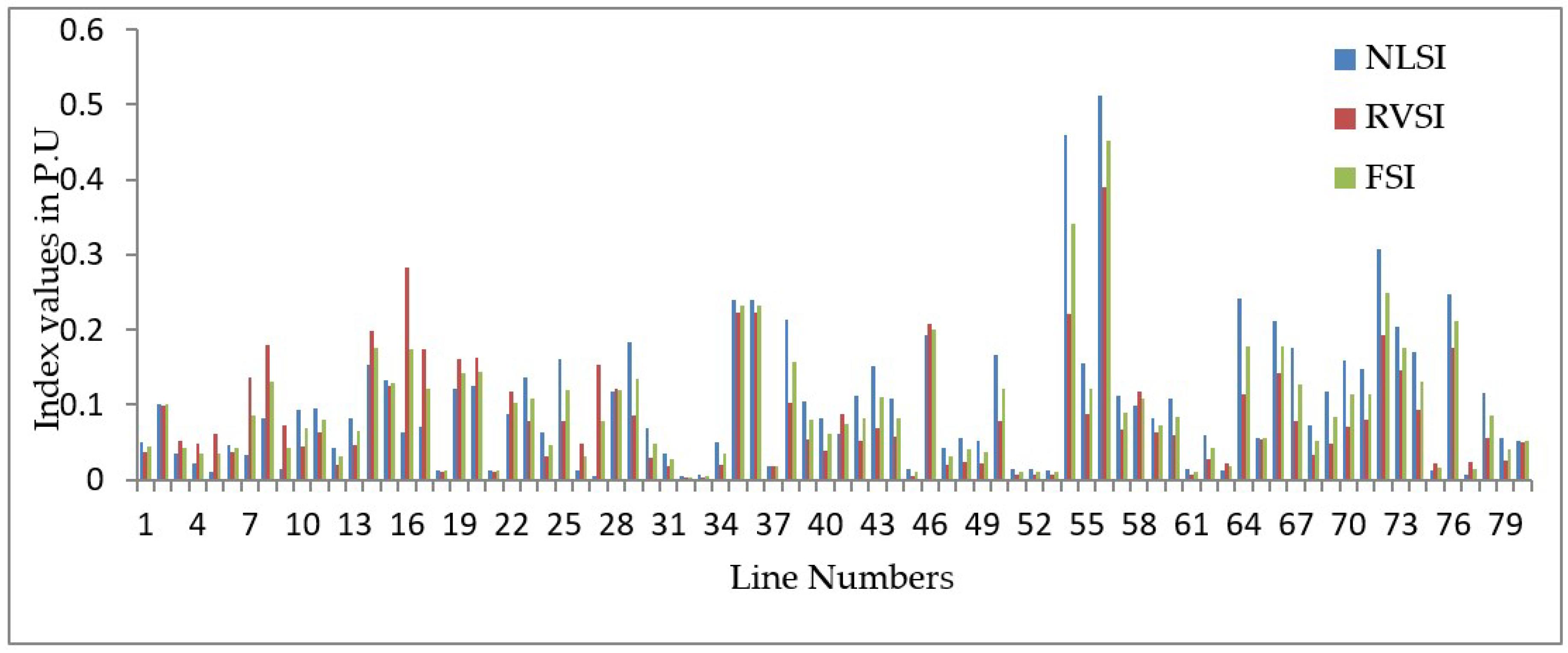
3. Index Based on Optimal Placement of TCSC

3.1. RapidVoltage Stability Index

To assess the voltage stability of an electrical power network, a rapid voltage stability index (RVSI) is taken to indicate a system’s weakness and susceptibility to voltage collapse [28]:
R V S I i j = 4 X i j V i 2 ( P j 2 Q j + Q j )
RVSIij = RVSI for the line associated with bus i and bus j. A heavily loaded line has a RVSI magnitude close to unity. Hence, RVSI values are kept at less than unity to ensure system stability.

3.2. Novel Line Stability Index

To determine the congestionof transmission lines and line capacity utilization, a novel line stability index(NLSI) is taken as [29]:
N L S I i j = R i j P j + X i j Q j 0.25 V i 2
NLSI gives an estimate of the percentage of the line being utilized.

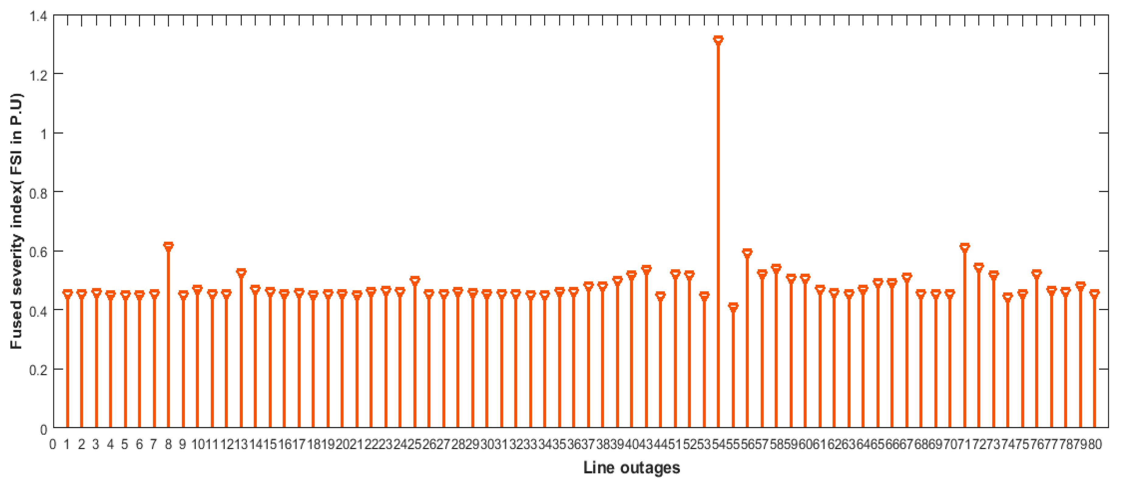
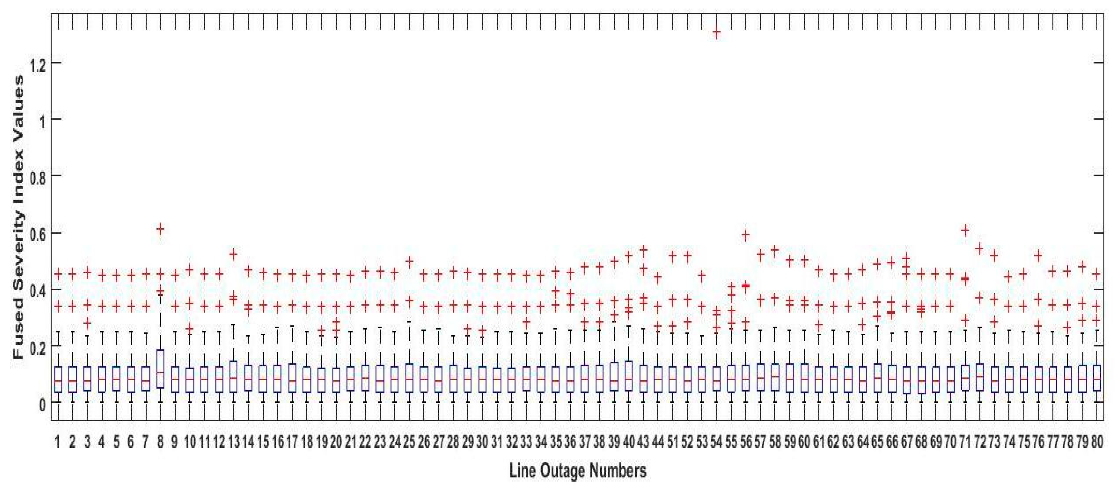
3.3. FusedSeverity Index

A fused index is formulated as a combination of NLSI and RVSI index set by the following balanced equation:
FSI = m1 × NLSI + m2 × RVSI
where m1 = m2 = 0.5.

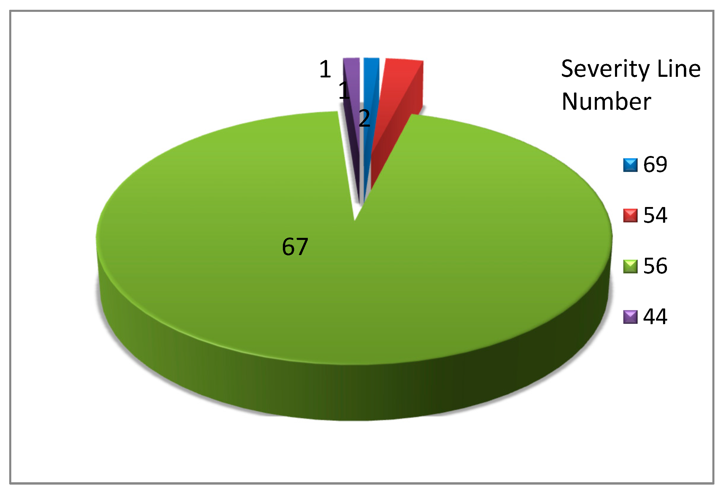
3.4. Intermittent Severity Index

After performing the contingency analysis, the intermittent severity index (IMSI) is determined to find a better location for the placement of TCSC. In this analysis, primarily the highest value of FSI for a specific line among all line contingenciesis determined. Then the number of times that line has been repeated in the line outages is identified. Lastly, the value of IMSI for a particular line can be obtained by multiplying the maximum value of FSI of that line for different line outages and the number of times that particular line has appeared in the severity list. The same procedure is repeated for all the lines. The linethat is having the highest value of IMSI is considered as the most severe line:
I M S I i j = P B i j × F S I i j M A X
IMSIij and FSIijMax are intermittent severity index and maximum fused severity index of the line between the i-th and j-th bus.

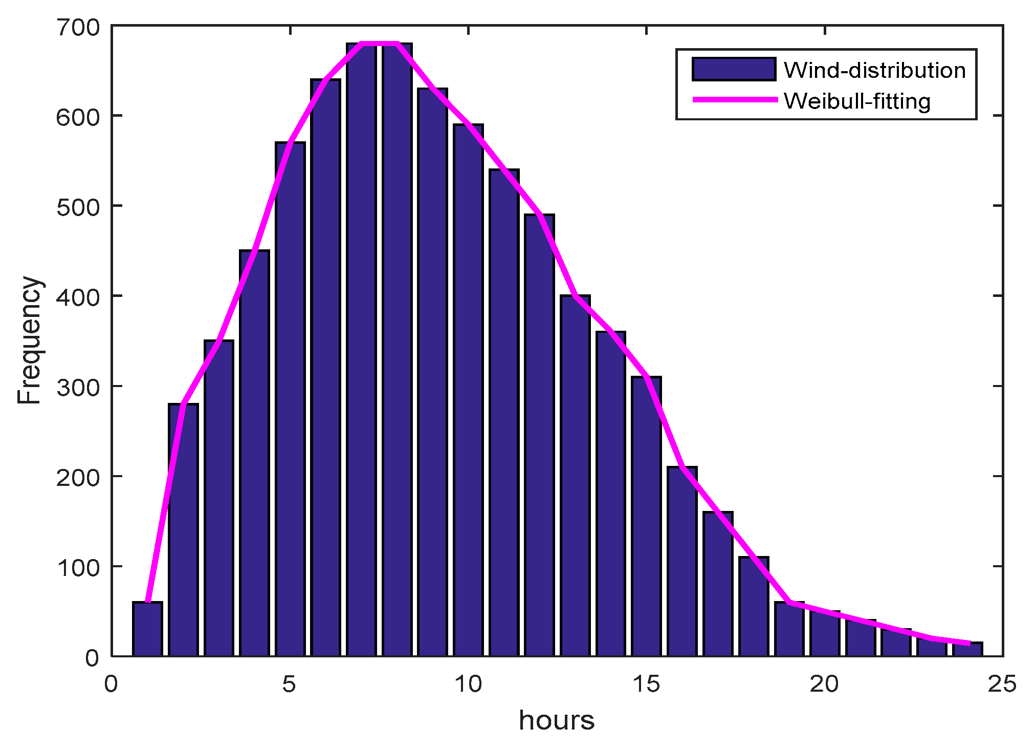
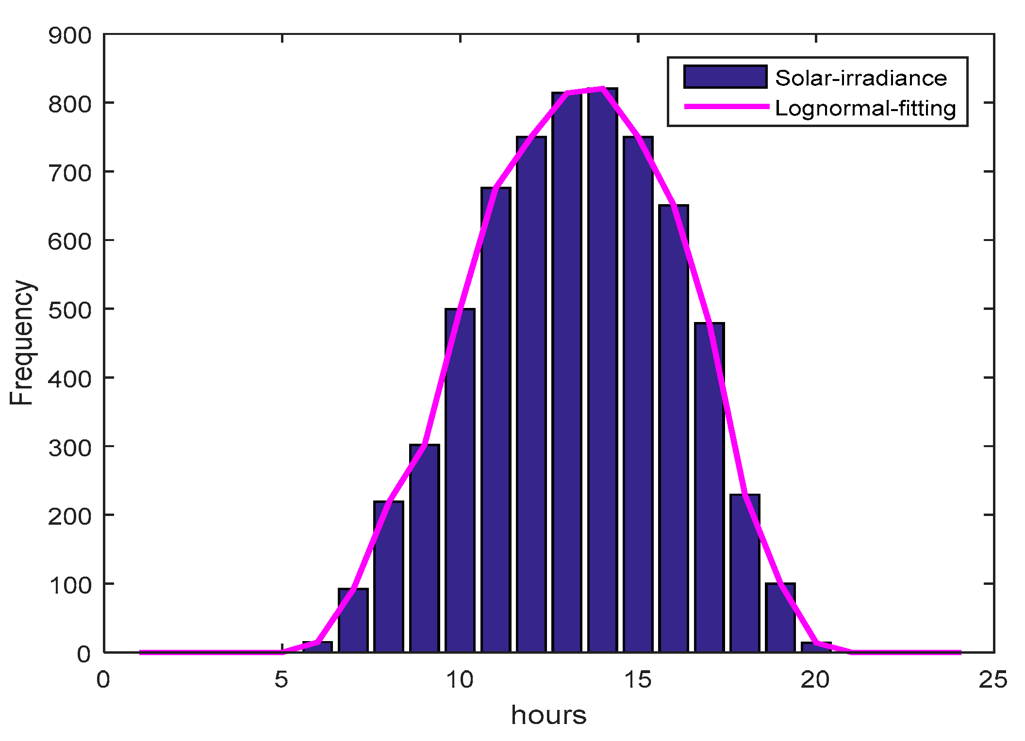
4. Weibull and Lognormal for Wind/PV

To assess the output power of wind, the Weibull PDF is used. In the Weibull study, the frequency, probability and cumulative probability are determined. The completeprocedure of the Weibull PDF is given below.

4.1. Weibull PDF

Here, the wind speed distribution is measured to utilize the Weibull PDF. In the Weibull, two parameters are used. The primary one is a scale constraint, and the second one is a shaped constraint. For the analysis of wind speed, the following Weibull distribution formula is given as:
f ( v ) = k c ( v c ) k 1 e ( v c ) k
where c and k denote the wind speed characteristics. If the c value is less the wind speed is also less. After that, the cumulative Weibull distribution is calculated by the succeeding function:
F ( v ) = 1 e ( v c ) k
Based on that, the cumulative Weibull distribution function is calculated, later the frequency is resolved. The wind power energy can be acquired by employing its power curve and represented by the succeeded equation:
P ( v ) = { 0 v < v c i o r v > v c o q ( v ) v c i v v r P r v r < v < v c o
Similarly, the lognormal function is examinedfor the PV power generation.

4.2. Lognormal PDF

In the section, the lognormal PDF function is used for the analysis of power in PV with random variable x. Lognormal distribution equation is given below with standard deviation and the mean:
f ( x : μ , β ) = { 1 β x 2 Π e 1 2 β 2 [ ln ( x ) μ ] 2 x 0 0 O t h e r w i s e
The density function for the analysis is represented as:
r ( x ) = 1 x β 2 Π e [ ln ( x ) μ ] 2 2 β 2
The mean and variance of the lognormal distribution is calculated as the following equation:
μ = e μ + β 2 2
β 2 = e 2 μ + β 2 ( e β 2 1 )
The lognormal distribution is used for anextensiveassortment of applications. It applied and assessed the output power of PV. Based on that, the frequency and probability of PV are analyzed. Here, the mean and variance values are changed; the relating values are assessed. The lognormal based PV is utilized to analyze the output power. After that, the variation of the mean and covariance parameters, the output power is resolved and accomplishes the optimal power flow solutions.

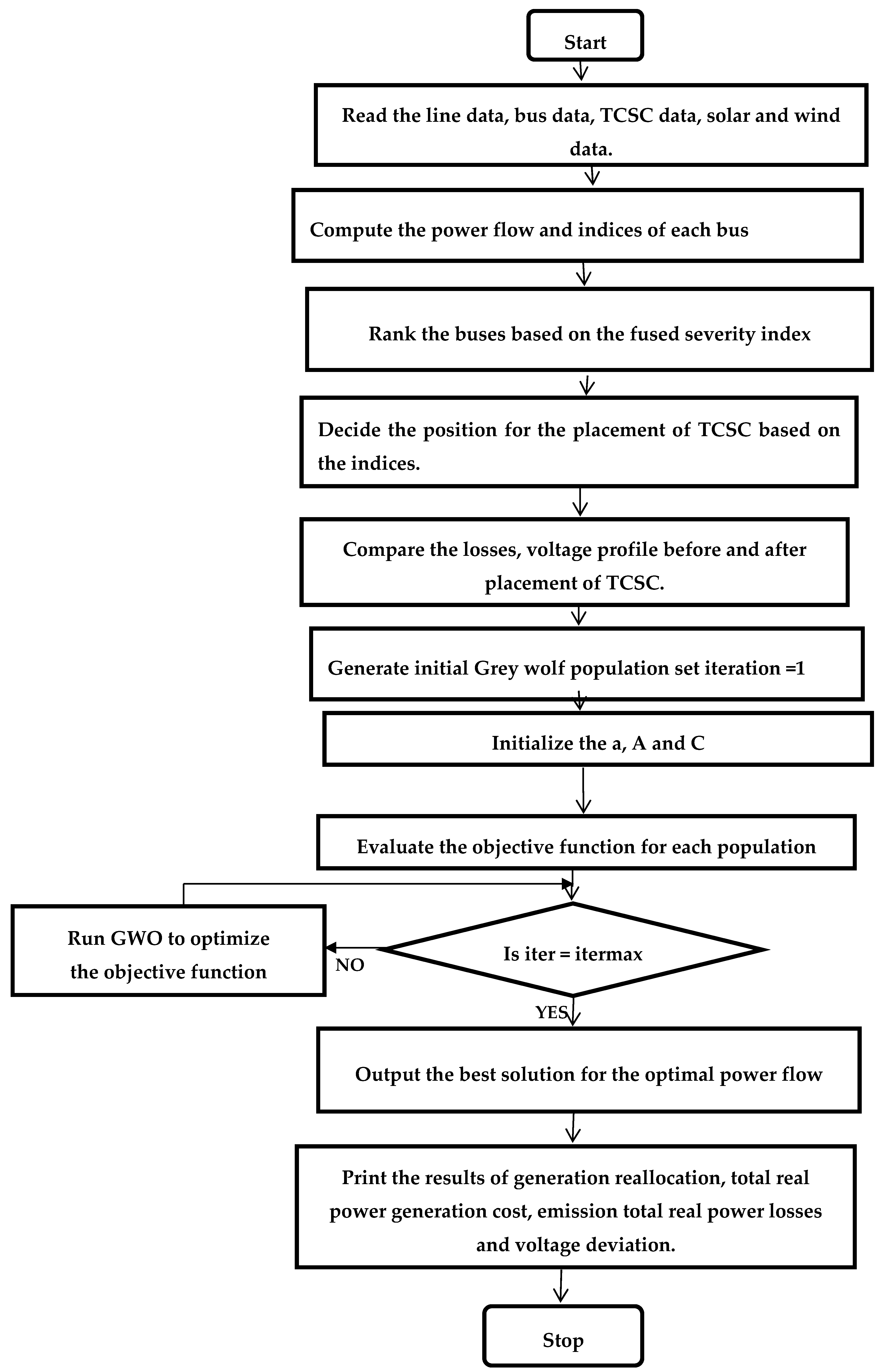
5. Optimal Tuning of TCSC using Grey Wolf Optimization

Mirjalilidescribed the grey wolf optimizer (GWO)algorithm in 2014 [27]; this procedure is wholly structured dependent on seeking prey and individual chasing agents of grey wolves. In this technique, four unique dimensions of chains of hierarchies are present. Grey wolves including ‘p’ being first then followed by the second one ‘q’ then third one ‘r’ and the last dimension ‘s.’Grey wolves are increasingly keen on living in a gathering. The pack size might be overall of around 5–12 wolves. Figure 1 depicts the flow chart for multi-objective function utilizing the grey wolf algorithm.
Algorithm 1. Grey Wolf Optimizer (GWO) Algorithms
1. Generate the initial prey wolf population/search agents
Yj (where j = 1, 2 ….n)
2. Initialize a, A and C
3. Compute the fitness value of each search agent
Yα = the best seek after an authority
Yβ = the second best seek after an authority
Yδ = the third best seek after an authority
4. Initialize Iteration = 1
5. Repeat the steps
6. For j = 1: Ys (size of Grey wolf)
For each chase agent
Invigorate the location of the current chase agent by using the equation
Y (k+1) = Y1 + Y2 + Y3/3
End for
7. Compute the fitness values of all chase agents
8. Renew the vectors of a, A and C
9. Renew the values of Yα, Yβ, Yδ
10. Increment the Iteration (k = k+1)
11. While (iterations< max number of iterations)
12. Get the output Yα
End

6. Simulation Results

An IEEE 57 bus system is amended to incorporate renewable energy system with equivalent values of thermal Generators. The grey wolf technique is used to resolve the OPF problem and check the effectiveness of the suggested method. Here 24h data is considered for the solar and wind power analysis [30]. The actual output power of the wind turbine is determined by using Weibull PDF and its variations of speed are noted. The wind speed is assumed as the miles per hour (m/h) and then it is converted into m/sec. Based on the Weibull PDF, the frequency is analyzed and plotted in Figure 2. Here, the output power flow of PV is investigated with the help of lognormal PDF functions. One PV is employed and the 24h PV data is noted. Based on the data, the irradiance level is noted and the corresponding frequency is determined and illustrated in Figure 3. The mean output power values of the wind farm and solar is assumed for solving the OPF and the proposed grey wolf algorithm has been implemented on IEEE-57bus system in the presence and absence of TCSC. Moreover, different cases like normal loading and contingency have been investigated and reported in separate tables to support the proposed method.

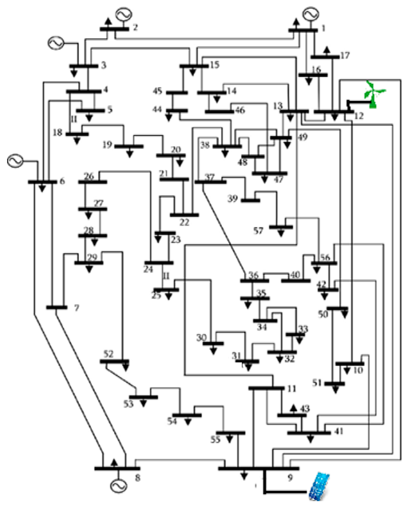
6.1. IEEE57 BusTest System

The modified IEEE 57 bus test system comprises of seven generators, among them slack bus is placed at bus 1 and four thermal generators are placed at the buses nos. 2,3,6,8, thesolar system is located at bus 9and wind system is located at bus no. 12 and the remaining 50 buses are treated as load buses. This configuration has 80 interconnected lines. The generator cost coefficient characteristics of IEEE57 bus have been presented in the Appendix A. Only load buses are assumed for the optimal placement of TCSC.Grey wolf optimization is utilized for obtaining the optimal power flow including and excluding TCSC and program is executed in MATLAB software and parameters are tabulated. Equal weights of 0.2 have been considered for all objectives. The results are carried out for different objective function.The Enercon model E82-E4 wind farm is chosen as the model connected to bus 12 andits datasheet is taken as reference for the analysis. The different speed values taken are vin = 3 m/s, vr = 12 m/s and vout = 25 m/s. Here 120 wind turbines, each with a rating of 3MWare considered to form a wind farm of 360 MW rating which gives amaximum output of 212 MW according to the Betz law. This value is taken output power of the wind farm. Solar park of 200 MW is considered for the radiation of 800 w/m2 in the standard climatic conditions. Table 1 represents the parameters of the grey wolf algorithm.

6.2. Normal Loading Condition

The different arrangements of weights related to NLSI and RVSI are altered and the obtained values are listed in Table 2. As the weighted values are changing the FSI value is decreasing.The weighted factors demonstrate the necessity of indices. The total value of NLSI is more than the value of the total value of NVSI further decrease in values is not desirable minimum values of total fused severity index has been observed for m1= −0.5 and m2 =0.5 and equal priority of indices has been selected for the calculations. Figure 4 shows NLSI, RVSI, FSI values for totally ranks of IEEE 57 bus system. Table 3 indicate that the top 25 RVSI, NLSI, and FSI values of all severity lines are listed in decrease order. From Table 3, it is noticed that line 56 connected between buses 41–43 has the highest FSI value. This location was chosen for the optimal placement for the TCSC based upon the highest fused severity index values. An additional node 58 is considered in between 41 and 43 for TCSC placement, and it is observed that losses, carbon emissions, fuel cost with valve-point effects are reduced at that particular location as compared to the placing TCSC at different positions of the IEEE 57 bus system as tabulated in Table 4. The system is tuned with a grey wolf algorithm by comprising the objective functions like generation fuel cost, active power losses, carbon emissions, fuel cost with valve-point effect and voltage deviations with and without TCSC. Table 5 and Table 6 indicate the different individual as well as multi-objective functions in the absence and presence of TCSC. It is observed that various parameters are reduced with TCSC placement at a particular location as compared to the without installation of TCSC. It is also noticed that the voltage profile is also improved.

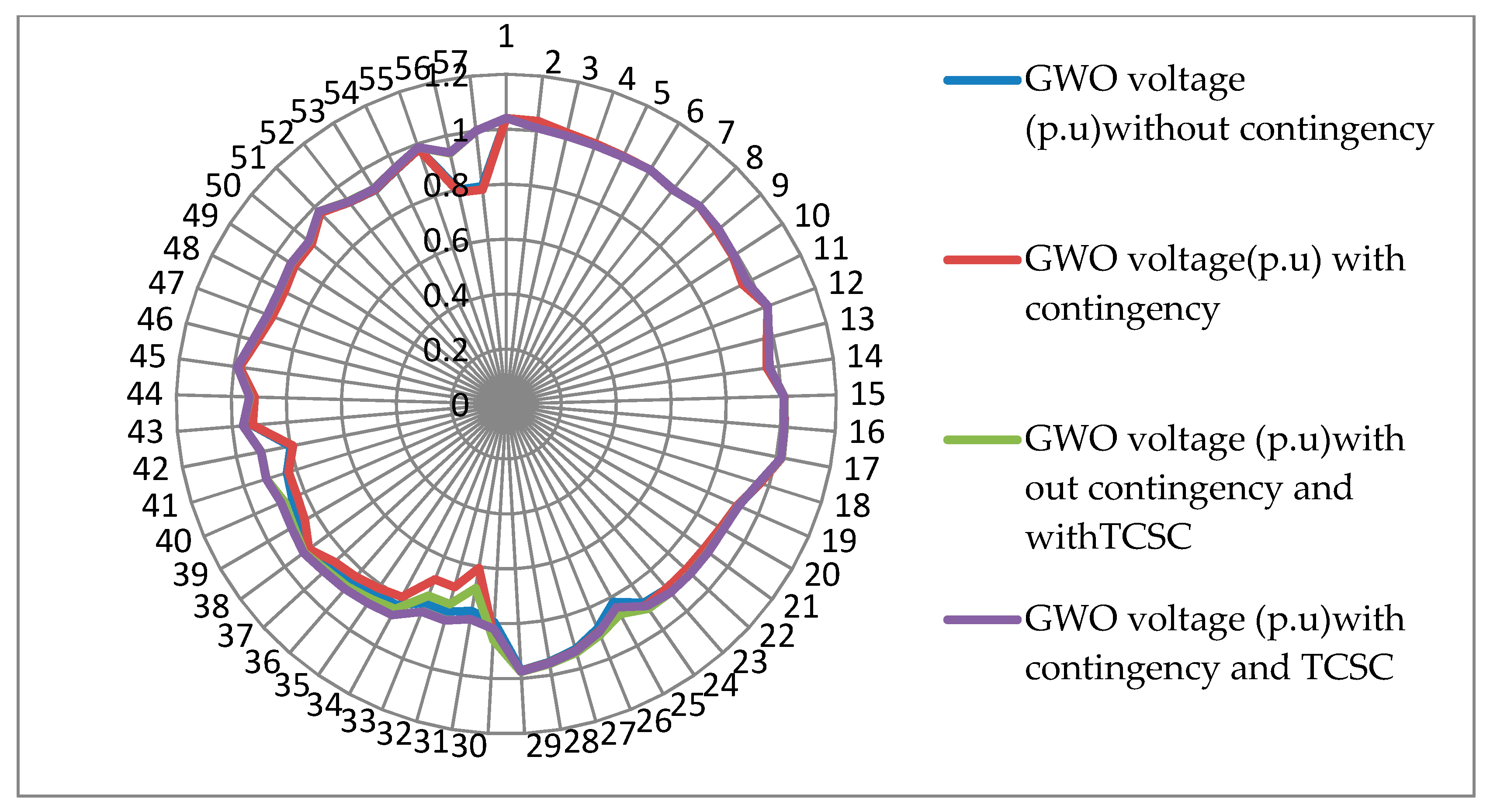
6.3. Contingency Condition using Intermittent Approach

The above system is also tested under contingency conditions using an intermittent method. The intermittent approach can be explained as the maximum value of FSI obtainedduring the line outages, multiplied by the number of times the probability of occurrence of the severity occurs in that line and is displayed in Figure 5. After the execution of contingency analysis, the intermittent severity index value can be determined to find out the better location for the placement of TCSC. Initially, the maximum value of the fused severity indexamong all the line outages is determined. Then the number of times that line was affectedis determined. The line with the highest value of the line outage is multiplied by the number of times the line has been repeated for many line outages is taken as reference. It is noticed from Table 7 that line number 56 is the most severe line that is associated with buses no. 41–43 causes more stress on the line. This line 56is removed and the load flow is done using Newtonraphson, this in turn gives the maximum severity value for line number 54, connected between buses 11–41, andhence TCSC is placed in line 54 under contingency conditions. This method provides a more accurate stressed line of the system as compared to the traditional way. The obtained maximum fused severity index values for distinctive line outages are represented as a stem plot shown in Figure 6. The box plot for (n-1) contingency of the modified IEEE 57 bus system is shown in Figure 7. The box plot shows all the FSI values taken for various line outages with maximum, minimum and median values. Table 8 gives the values for different parameters like own generators, real power generation, Active power loss, voltage deviation have been compared including and excluding contingency and TCSC. It is also further tuned with the grey wolf algorithm. Figure 8 indicates a marked improvement in the voltage profile of all buses without and with tuned TCSC under normal and contingency conditions. Table 9 and Table 10 consist of different objective functions in the presence and absence of TCSC with contingency.As compared to the Table 9 the objectives functions such as total generation cost, valve-point loading effect, voltage deviation, carbon-emission, active power loss present in Table 10 gave better results with optimal placement of TCSC using the grey wolf technique. The value of the individual objective function and multi-objective function effectively decreased with optimal placement of TCSC and enhanced the power transfer capability of the electrical network. It shows that the proposed grey wolf technique gives better results. Table A1 depicts the characteristics of the IEEE-57 bus system and cost coefficients of solar and wind are taken as 1.5$/h. Figure A1. Shows Integrated IEEE57 bus system with solar and wind

7. Conclusions

For any consistent and successful operation of integrated system generator reallocation, reducing the losses voltageand stability are the primary issues. A multi-objective function comprised of active power loss, generation fuel cost along with valve-point impact, voltage deviation carbon discharges, with the utilization of minimum value of TCSC is considered for the optimal tuning of TCSC using grey wolf optimization.
  • A fused severity index has been implemented for finding out the most stressed line of the transmission system.The weak lines are recognized based on the rank and arranged in descending order of fused severity index for the lines associated between the buses.
  • Uncertainties of solar and wind are demonstrated as lognormal and Weibull probabilistic distribution functions and their interconnectionsto the traditional grid are explained.
  • The TCSC and output of generators are additionally tuned by limiting a multi-objective function comprising of active power loss, fuel cost with valve-point effect, carbon dischargesutilizing grey wolf algorithm and the best global ideal values are achieved.
  • A reduction in the losses, carbon discharges, fuel cost with valve-point effect has been obtained with an improvement in the voltage profile of the integrated system. The reduction in active power loss helps in contingency management. Improvement of voltage deviation helps in protectingthe system against line outages.
  • Finally, it can be inferred that the explored strategy is more capable in decreasing the losses, carbon emission and improving the voltage profile.

Author Contributions

Investigation, M.R.; Supervision, G.V.N.K. and S.S.

Funding

This research received no external funding.

Conflicts of Interest

The authors declare no conflict of interest.

Abbreviations

Nomenclature
TCSCThyristor-Controlled Series Compensator
SBSending end bus
RBReceiving end bus
RVSIRapid Voltage Stability Index
NLSINovel Line Stability Index
FSIFused Severity Index.
PDFProbability Density Function
GWOGrey Wolf Optimizer
FACTSFlexible AC Transmission System
VDVoltage Deviation
VPEValve Point Effect
CECarbon Emissions
IMSIIntermittent Severity Index
OPFOptimal Power Flow
PVPhoto Voltaic
SVCStatic VAR Compensator
Symbols
PweWind power generation from eth bus
PsfPower output from the fth PV plant
PLOverall real power loss
QLOverall reactive power loss,
PGiReal power generated in ith bus
PDiReal power demanded in ithbus
P TGI min The minimum power of the ith thermal unit
PjActive power at receiving at jth bus
QjReactive power at receiving at jth bus
NTGNumber of generator buses
a, b, cFuel cost coefficients
VkMagnitude of voltage at bus k
XReactance of line
XTCSCReactance of the TCSC
VinWind Speed (Cut-in)
VCOWind Speed (Cut-out)
VrWind Speed (Rated)
PrRated Power
ntlNo. of lines for transmission
Nno of buses
Zimpedance of line in ohms
geDirect cost coefficient of the eth wind farm
hfDirect cost coefficient of the fth solar plant
R i j The resistance of the line
SijApparent power flowing in the line
VkrefMagnitude of the Reference voltage at the busk
di,eiValve-Point Effect Coefficient
δi, φi, λi, ψi, σiEmission coefficients
cScale Parameter
kShape Parameter
PBijProbability occurring of line ij for all contingencies of the system
Βvariance of the lognormal distribution
µMean of the lognormal distribution
w1,w2, w3, w4, w5, m1, m2Weighted factors

Appendix A

Table A1. Generator Characteristics of IEEE 57 Bus Systems.
Generator Bus No.a ($/MW2/h)b ($/MW/h)c ($/h) P G m i n   ( MW ) P G m a x   ( MW ) δiφiλiψiσidiei
10.0775200019754.091−5.550.5490.00020.286180.037
20.0140001002.543−6.040.46380.00050.333160.038
30.2520001406.131−5.550.41510.000010.66713.50.041
60.140001003.491−5.750.5390.00030.266180.037
80.0222220005504.258−5.090.35860.0000010.8140.04
Figure A1. Integrated IEEE57 bus system with solar and wind.
Energies 12 02215 g0a1

References

  1. Ogunjuyigbe, A.S.O.; Ayodele, T.R.; Akinola, O.A. Optimal allocation and sizing of PV/Wind/Split-diesel/Battery hybrid energy system for minimizing life cycle cost, carbon emission and dump energy of the remote residential building. Appl. Energy 2016, 171, 153–171. [Google Scholar] [CrossRef]
  2. Kusakana, K. Optimal scheduled power flow for distributed photovoltaic/wind/diesel generators with battery storage system. IET Renew Power Gener. 2015, 9, 916–924. [Google Scholar] [CrossRef]
  3. Sanseverino, E.R.; Di Silvestre, M.L.; Badalamenti, R.; Nguyen, N.Q.; Guerrero, J.M.; Meng, L. Optimal power flow in islanded microgrids using a simple distributed algorithm. Energies 2015, 8, 11493–11514. [Google Scholar] [CrossRef]
  4. Erdinc, O.; Uzunoglu, M. Optimum design of hybrid renewable energy systems: Overview of different approaches. Renew Sustain. Energy Rev. 2012, 16, 1412–1425. [Google Scholar] [CrossRef]
  5. Deng, W.; Zhang, B.; Ding, H.; Li, H. Risk-based probabilistic voltage stability assessment in an uncertain power system. Energies 2017, 10, 180. [Google Scholar] [CrossRef]
  6. Shadmand, M.B.; Balog, R.S. Multi-objective optimization and design of a photovoltaic-wind hybrid system for community smart DC microgrid. IEEE Trans. Smart Grid 2014, 5. [Google Scholar] [CrossRef]
  7. Rambabu, M.; Nagesh Kumar, G.V.; Siva Nagaraju, S. Energy management of microgrid using support vector machine (SVM) model. IIOAB J. 2016, 7, 116–132. [Google Scholar]
  8. Carvallo, J.P.; Shaw, B.J.; Avila, N.I.; Kammen, D.M. Sustainable Low-Carbon Expansion for the Power Sector of an Emerging Economy: The Case of Kenya. Environ. Sci. Technol. 2017, 51, 10232–10242. [Google Scholar] [CrossRef] [Green Version]
  9. Abaci, K.; Yamacli, V. Differential search algorithm for solving multi-objective optimal power flow problem. Int. J. Electr. Power Energy Syst. 2016, 79, 1–10. [Google Scholar] [CrossRef]
  10. Shi, L.; Wang, C.; Yao, L.; Ni, Y.; Bazargan, M. Optimal power flow solution incorporating wind power. IEEE Syst. J. 2012, 6, 233–241. [Google Scholar] [CrossRef]
  11. Sichilalu, S.; Mathaba, T.; Xia, X. Optimal control of a wind–PV-hybrid powered heat pump water heater. Appl. Energy 2017, 185, 1173–1184. [Google Scholar] [CrossRef]
  12. Levron, Y.; Guerrero, J.M.; Beck, Y. Optimal Power Flow in MicrogridsWith Energy Storage. Power Syst. IEEE Trans. 2013, PP, 1–9. [Google Scholar] [CrossRef]
  13. Biswas, P.P.; Suganthan, P.N.; Amaratunga, G.A.J. Optimal power flow solutions incorporating stochastic wind and solar power. Energy Convers. Manag. 2017, 148, 1194–1207. [Google Scholar] [CrossRef]
  14. HamzehAghdam, F.; Salehi, J.; Ghaemi, S. Contingency based energy management of multi-microgrid based distribution network. Sustain. Cities Soc. 2018, 41, 265–274. [Google Scholar] [CrossRef]
  15. Rao, V.B.; Engineering, E.; Kumar, G.V.N.; Engineering, E. A Comparative Study of BAT and Firefly Algorithms for Optimal Placement and Sizing of Static VAR Compensator for Enhancement of Voltage Stability. Int. J. Energy Optim. Eng. 2015, 4, 68–84. [Google Scholar] [CrossRef]
  16. Hingorani, N.G.; Gyugyi, L.; El-Hawary, M. Understanding FACTS—Concepts and Technology of Flexible AC Transmission Systems; Wiley-IEEE Press: Hoboken, NJ, USA, December 1999. [Google Scholar]
  17. Bali, S.K.; Munagala, S.; Gundavarapu, V.N.K. Harmony search algorithm and combined index-based optimal reallocation of generators in a deregulated power system. Neural Comput. Appl. 2017, 1–9. [Google Scholar] [CrossRef]
  18. Kumar Gundavarapu, V.N.; Mishra, A. Line utilization factor-based optimal allocation of IPFC and sizing using firefly algorithm for congestion management. IET Gener. Transm. Distrib. 2016, 10, 115–122. [Google Scholar] [CrossRef]
  19. Modarresi, J.; Gholipour, E.; Khodabakhshian, A. A comprehensive review of the voltage stability indices. Renew Sustain. Energy Rev. 2016, 63, 1–12. [Google Scholar] [CrossRef]
  20. Kim, S.S.; Kim, M.K.; Park, J.K. Consideration of multiple uncertainties for evaluation of available transfer capability using fuzzy continuation power flow. Int. J. Electr. Power Energy Syst. 2008, 30, 581–593. [Google Scholar] [CrossRef]
  21. Nireekshana, T.; KesavaRao, G.; SivanagaRaju, S. Available transfer capability enhancement with FACTS using Cat Swarm Optimization. Ain Shams Eng. J. 2016, 7, 159–167. [Google Scholar] [CrossRef] [Green Version]
  22. Samimi, A.; Naderi, P. A New Method for Optimal Placement of TCSC Based on Sensitivity Analysis for Congestion Management. Smart Grid Renew. Energy 2012, 2012, 10–16. [Google Scholar] [CrossRef]
  23. Bhattacharyya, B.; Gupta, V.K. SVC & TCSC for Minimum Operational Cost Under Different Loading Condition. 2012, pp. 1–6. Available online: www.iitk.ac.in/npsc/Papers/NPSC2012/papers/12055.pdf. (accessed on 26 June 2018).
  24. Mukherjee, A.; Mukherjee, V. Solution of optimal power flow using chaotic krill herd algorithm. Chaos Solit. Fract. 2015, 78. [Google Scholar] [CrossRef]
  25. Vlachogiannis, J.G.; Lee, K.Y. A comparative study on particle swarm optimization for optimal steady-state performance of power systems. IEEE Trans. Power Syst. 2006, 21, 1718–1728. [Google Scholar] [CrossRef]
  26. Daryani, N.; Hagh, M.T.; Teimourzadeh, S. Adaptive group search optimization algorithm for multi-objective optimal power flow problem. Appl. Soft Comput. J. 2016, 38, 1012–1024. [Google Scholar] [CrossRef]
  27. Mirjalili, S.; Mirjalili, S.M.; Lewis, A. Grey Wolf Optimizer. Adv. Eng. Softw. 2014, 69, 46–61. [Google Scholar] [CrossRef] [Green Version]
  28. Murty, V.V.S.N.; Kumar, A. Optimal placement of DG in radial distribution systems based on new voltage stability index under load growth. Int. J. Electr. Power Energy Syst. 2015, 69, 246–256. [Google Scholar] [CrossRef]
  29. Yazdanpanah-Goharrizi, A.; Asghari, R. A Novel Line Stability Index (NLSI) for Voltage Stability assessment of Power Systems. In Proceedings of the 7th WSEAS e 7th WSEAS International Conference on Power Systems, Beijing, China, 15–17 September 2007; pp. 164–167. [Google Scholar]
  30. Fort Collins Data Access: Results. Available online: http://climate.colostate.edu/~autowx/fclwx_results.php (accessed on 26 June 2018).
Figure 1. Flow chart for multi-objective optimization using grey wolf algorithm.
Energies 12 02215 g001
Figure 2. Frequency analysis-based wind speed (k = 3, c = 6).
Energies 12 02215 g002
Figure 3. Illustrations of frequency for solar (mean = 2, SD = 3) variation.
Energies 12 02215 g003
Figure 4. NLSI, RVSI and FSI values of all lines in IEEE-57-bus system.
Energies 12 02215 g004
Figure 5. Probability of occurrence severity lines in IEEE-57-bus system.
Energies 12 02215 g005
Figure 6. Maximum fused severity index values for various line outages.
Energies 12 02215 g006
Figure 7. Box plot for fused severity index values for various line outages.
Energies 12 02215 g007
Figure 8. Voltage profile for the IEEE 57 bus system including and excluding TCSC.
Energies 12 02215 g008
Table 1. Grey wolf algorithm parameters.
Serial Number.ParametersQuantity
1Grey wolf size20
2Number of iterations50
3a vector2
Table 2. A contrast of FSI of the system for various weights.
m1(NLSI)m2(NVSI)Total FSI
0.50.57.3884
0.60.47.5503
0.70.37.7122
0.80.27.8741
0.90.18.036
Table 3. NLSI, RVSI and FSI Values of top 25 lines in IEEE-57-bus system.
LINE NumbersSB NumberRB NumberNLSI (p.u.)RVSI(p.u.)FSI(p.u.)
5641430.51230.39050.4514
161160.06330.28360.3404
3524250.23930.22350.2494
3624250.23930.22350.2314
5411410.45930.22140.2314
4634320.19230.20790.2119
1413150.1540.19840.2001
7244450.30660.19220.1777
8890.08120.18020.177
7639570.24690.17680.1762
171170.0710.17350.175
204180.12490.1620.1734
194180.12230.16180.1575
2712170.00410.15350.1435
7340560.20460.14530.1421
6613490.21160.14230.1349
7680.03390.13590.1313
151150.13220.12440.1307
281150.11690.12130.1283
5815450.09840.11810.1267
22780.08810.1170.1223
6450510.24130.11410.1223
3826270.21280.10230.1221
2230.10110.09910.1194
Table 4. Multi-objective function in IEEE 57 bus system by locating TCSC in differentplaces.
SB NumberRB NumberTotal Power Generation (MW)Fuel Cost ($/h)Active Power Losses(MW)Emission(t/h)Voltage Deviation in p.uValve Point Effect ($/h)Multi-Objective Function
41431227.22748731.411.00644.8522753411012
1141122742752131.59751.04574.83382755811023
1315122792751532.07671.05934.9122755711022
4445122782748531.9551.02764.93042754011013
50511227.32748931.18771.00654.85262753711014
Table 5. Optimal Power flow solution without contingency using GWO.
ParameterOF1OF2OF3OF4OF5OF6
Real power generation (MW)PG1(MW)158.0297265.076163.4177179.0372170.1787165.5765
PG2(MW)10012.8868100100100100
PG3(MW)49.4902125.90349.913814014051.4046
PG6(MW)18.184106.12815.762515015014.9543
PG8(MW)490.8169301.122487.1829243.1543251.931484.1597
PGs(MW)200200200200200200
PGw(MW)210210210210210210
Total Active power generation (MW)1226.5211221.121226.27691222.1921222.111226.095
Total real power generation cost ($/h)273433176927347329073276227352
Active power Loss (MW)30.7225.31630.4726.3926.3130.29
Valve point effect cost ($/h)273933181527391329463279927393
Voltage deviation (p.u.)4.90584.79124.89964.764.84.8951
Carbon Emission(ton/h)1.01590.79451.01240.59240.59111.0479
Objective function2734325.316273914.760.591110956
Computation time27.9926.9923.6823.9822.7623.44
OF1: Generation cost, OF2: Active power Loss, OF3: Valve point effect cost, OF4: Voltage Deviation, OF5: Carbon emissions, OF6: Multiobjective function.
Table 6. Optimal Power flow solution without contingency with TCSC using GWO.
ParameterOF1OF2OF3OF4OF5OF6
Real power generation (MW)PG1(MW)171.6265265.1003176.1099324.9398174.6181184.4858
PG2(MW)10029.0587100100100100
PG3(MW)47.329592.225347.875822.322314048.5226
PG6(MW)16.8781114.228512.063952.221158.73166.2416
PG8(MW)479.7787309.8535479.4983314.4824239.0236476.0984
PGs(MW)200200200200200200
PGw(MW)210210210210210210
Total Active power generation (MW)1225.6131220.4661225.5481223.9661222.3731225.348
Total real power generation cost ($/h)265803003226582304233240926603
Active power Loss (MW)29.81224.6629.7428.16526.5729.5484
Valve point effect($/h)266293007026626304613244426635
Voltage deviation (p.u.)4.82674.7944.82474.77944.8084.8206
Carbon Emission(ton/h)0.96660.79360.97270.95240.55620.9755
Objective function2658024.66266264.77940.556210655
Computation time(secs)26.7625.8424.4321.6425.2627.41
Table 7. Contingency analysis by intermittent approach.
(Max FSI) x(No of Times the Severity of the Line)Intermittent Index Value(p.u)Severity Line No.SBRB
0.5083230.508323695354
0.6100*21.22541141
0.614*6741.138564143
0.5375430.537543443132
Table 8. Different parameters for the IEEE57bus system using the grey wolf algorithm.
QuantityTuned Without Contingency and TCSCTuned Without Contingency and with TCSCTuned with Contingency and without TCSCTuned with Contingency and TCSC
Real power generation (MW)PG1(MW)165.576184.4858152.2136192.0006
PG2(MW)100100100100
PG3(MW)51.404648.522649.331347.9692
PG6(MW)14.95436.241616.516413.7667
PG8(MW)484.159476.0984501.8825464.311
PGs(MW)200200200200
PGw(MW)210210210210
Total power generation (MW)1226.091225.351229.9441228.048
Total Load(MW)1195.81195.81195.81195.8
Active power Loss (MW)30.2925.6234.143832.2475
Voltage deviation (p.u.)4.89514.776.17096.1562
Table 9. Optimal power flow solution with contingency using GWO.
ParameterOF1OF2OF3OF4OF5OF6
Real power generation (MW)PG1(MW)160.8007253.576164.1703236.6245164.3258152.2136
PG2(MW)1009.0711100100100100
PG3(MW)50.032414051.086114014049.3313
PG6(MW)16.8994103.687217.96143.98915016.5164
PG8(MW)491.5837307.4762485.7775335.7361260.4213501.8825
PGs(MW)200200200200200200
PGw(MW)210210210210210210
TotalActivepowergeneration (MW)1229.3161223.8111228.9951226.351224.7471229.944
Total real power generation cost ($/h)27467322062747130867327627472
Active power Loss (MW)33.5128.0133.1930.5428.9434.1438
Valve point effect($/h)275163223527515309093280427529
Voltage deviation (p.u.)6.0975.9626.095.94115.94566.1109
Carbon Emission(t/h)1.02330.78791.00960.79530.59581.0449
Objective function2746728.01275155.94110.595811008
Computation time(s)26.1327.729.226.8927.0124.01
Table 10. Optimal power flowsolution with contingency and TCSC using GWO.
ParameterOF1OF2OF3OF4OF5OF6
Real power generation (MW)PG1(MW)154.0963269.203156.1643329.2276158.5345172.0006
PG2(MW)10029.692100100100100
PG3(MW)47.764495.238648.119421.156414047.9692
PG6(MW)36.5722115.824934.285852.4674158.637713.7667
PG8(MW)480.4047303.6558480.2326314.3568238.3618464.311
PGs(MW)200200200200200200
PGw(MW)210210210210230230
Total active power generation (MW)1228.8381223.6141228.8021227.2081225.5341228.048
Total real power generation cost ($/h)267193040326721307103255526759
Active power Loss (MW)33.0327.81433.002131.408229.7332.2475
Valve point effect($/h)267673044926765307443258826795
Voltage deviation (p.u.)6.16816.13036.1676.11436.14746.1562
Carbon emission(ton/h)0.97280.79620.97550.96740.56140.95
Objective function2671927.814267656.11430.561410719
Computation time(secs)27.6823.9226.10425.0925.9822.89

