You are currently viewing a new version of our website. To view the old version click .
Energies
  • Article
  • Open Access

11 June 2019

Energy Saving Operation of Manufacturing System Based on Dynamic Adaptive Fuzzy Reasoning Petri Net

,
,
and
1
Department of Industrial and Manufacturing System Engineering, Huazhong University of Science and Technology, Wuhan 430074, China
2
Department of Mechanical and Aerospace Engineering, University of Virginia, Charlottesville, VA 22904 USA
*
Author to whom correspondence should be addressed.
This article belongs to the Special Issue Energy Efficiency of Manufacturing Processes and Systems

Abstract

The energy efficient operation of a manufacturing system is important for sustainable development of industry. Apart from the device and process level, energy saving methods at the system level has attracted increasing attention with the rapid growth of the industrial Internet of things technology, which makes it possible to sense and collect real-time data from the production line and provide more opportunities for online control for energy saving purposes. In this paper, a dynamic adaptive fuzzy reasoning Petri net is proposed to decide the machine energy saving state considering the production information of a discrete stochastic manufacturing system. Fuzzy knowledge for energy saving operations of a machine is represented in weighted fuzzy production rules with certain values. The rules describe uncertain, imprecise, and ambiguous knowledge of machine state decisions. This makes an energy saving sleep decision in advance when a machine has the inclination of starvation or blockage, which is based on the real-time production rates and level of connected buffers. A dynamic adaptive fuzzy reasoning Petri net is formally defined to implement the reasoning process of the machine state decision. A manufacturing system case is used to demonstrate the application of our method and the results indicate its effectiveness for energy saving operation purposes.

1. Introduction

It has been shown that 37% of the energy consumption and 17% of carbon dioxide (CO2) emissions come from the industrial sector [1]. Moreover, the energy consumption of industries has an annual growth rate of 1.3% from 2013 to 2025 [2]. The manufacturing industry is responsible for 38% of energy-related CO2 emissions in China [3]. Its sustainable development requires industries to improve their energy efficiency eagerly [4,5]. The International Energy Agency reported that approximately 18–26% of the total energy consumption in manufacturing industries, i.e., 25-37 EJ, can be saved if proper actions are taken [6]. The energy-saving potential in manufacturing industries worldwide is estimated to be 20% until 2050 [7]. Therefore, energy management decisions are more and more important for manufacturing industries all over the world [8].
It is known that idle states are common in the shift time of non-bottleneck machines. The idle period took over 16% of the production time in an aircraft small-parts supplier and there was a turn-off opportunity to save at least 13% of the total energy consumption [9]. Apparently, the status of machines in a manufacturing system should be continuously monitored to make a decision. An OFF/SLEEP action could be taken for energy saving when a machine becomes idle (or tends to be idle). Later, it should be switched on or woken up to recover the production at an appropriate time slot without sacrificing the system throughput.
The development of the industrial internet of things (IoT) has endowed modern manufacturing systems with the sensible ability and real-time production data which can be collected, and provides more opportunities for energy saving operations. Currently, many new computerized numerical control (CNC) machines and robotics have energy-saving modes. However, most manufacturing execution systems have no module or function for energy saving decisions. From the system level, many works focus on the scheduling of jobs to minimize non-processing energy consumption [10]. Research on the dynamic decision of machine states for energy efficient manufacturing have gradually received significant attention from academics and industries.
The paper is organized as follows: Some related literatures are reviewed in Section 2. Section 3 describes the energy saving operations of a manufacturing system and the knowledge representation of machine state reasoning based on weighted fuzzy production rules are proposed. Section 4 proposes a dynamic adaptive fuzzy reasoning Petri net for machine state inferences to save energy considering the real-time production information. In Section 5, a serial manufacturing system is studied to demonstrate the effectiveness of our method and some discussions are also provided. Conclusions and future works are discussed in Section 6.

3. Problem Statement and Fuzzy Operation Knowledge Representation

3.1. System Description and Assumptions

For a serial discrete manufacturing system (Figure 1) in this paper, the assumptions are made in time (0,T] as follows.
Figure 1. A multistage serial manufacturing system.
  • Machine Mi, i = 1, 2, …, n, has a constant cycle time τ i . The cycle time of machines can be the same or different, which means the system can be synchronous or asynchronous lines.
  • Buffer Bi, i = 1, 2, …, n−1, has a finite buffer capacity Li. The buffer level of Bi at time t is represented as bi(t) at the beginning of each discrete time slot.
  • The reliability models of machines are assumed to follow a known but not definitive probability distribution. The time dependent failure mode is used in this study.
  • At the beginning of a discrete time slot, Mi is starved if it is powered on and its upstream buffer Bi-1 is empty. It is assumed that the first machine is never starved.
  • At the beginning of a discrete time slot, Mi is blocked if it is powered on and its downstream buffer Bi is full. It is assumed that the last machine is never blocked.
  • A power-on machine consumes materials, such as electricity, fuel, gas and compressed air. All consumed materials will be converted into energy.
  • In this study, a machine has following states: Processing (PS), starvation (ST), blockage (BL), failure (FL), and sleep for energy saving (SL).
In a time unit, a machine in a processing state consumes the processing energy Eps,i. The energy consumption of traditional idle states, i.e., starvation and blockage, is described as Eid,i. A machine consumes energy Esl,i in the energy saving state, i.e., sleep state. It is assumed that Esl,i < Eid,i < Eps,i. A machine in a failure state does not consume energy. Buffers do not consume energy. The consumed energy Ei of a machine Mi in time (0,T] is calculated as:
E i ( T ) = E p s , i × T p s , i + E i d , i × T i d , i + E s l , i × T s l , i ,
where Tps,i, Tid,i, Tsl,i are the time length of the corresponding machine state.
The overall energy consumption of a manufacturing system Esys during time (0,T] is the summation of the energy consumption of all machines as follows:
E s y s ( T ) = i = 1 n E i ( T ) ,
Based on Esys, the total energy cost of machines in a manufacturing system can be achieved. In this paper, the total energy cost of machines, the system throughput and the energy consumption per part are the main energy performance indicators of a manufacturing system.

3.2. Knowledge Representation of Machine Energy Saving Operations

The machine idle states are the main non-valuable operational states with higher energy consumption. Reducing or eliminating the idle periods by switching a machine into the energy saving state for some reasonable duration, and then waking it up, is the main objective of our work. Regarding a power-on machine, the decision of whether or not to switch it into the sleep state is evaluated and executed between two consecutive time slots based on production data. If a sleep operation is decided, the machine enters the sleep state during the subsequent time period. If a running decision is made, the machine is woken up from the sleep state or keeps its running state.
Traditionally, an exact buffer level was assigned as the threshold value for switching ON/OFF a machine that approaches either starvation (due to upstream buffer) or blockage (due to downstream buffer) [14,15]. It is difficult to decide a precise level of all buffers for energy control purposes in different manufacturing systems due to the combinatorial explosion of the buffer levels. Fuzzy production rules (FPRs) are a good tool for processing uncertain, imprecise, ambiguous real-world knowledge, and the uncertainty of the fulfillment of the conditions in rules [27]. Fuzzy knowledge representations for energy saving machine operation based on weighted FPRs (WFPRs) is presented in this study to switch a machine into the energy saving state in advance, if the machine has an inclination of starvation or blockage based on the real level of its upstream buffer, downstream buffer and production rate.
Let Rx be a set of WFPRs for machine state reasoning. Based on the definition of a general WFPR [37], a specific WFPR for the energy saving operation of a power-on machine is described in this paper as follows:
R x : IF   b i ( t )   is   U B   AND   b i + 1 ( t )   is   D B   THEN   s i ( t )   is   S R   ( c f i ( t ) = μ x ) ,   ω u b , x ,   ω d b , x ,
where
  • bi(t) is the level of upstream buffer of Mi at time point t.
  • bi+1(t) is the level of downstream buffer of Mi at time point t.
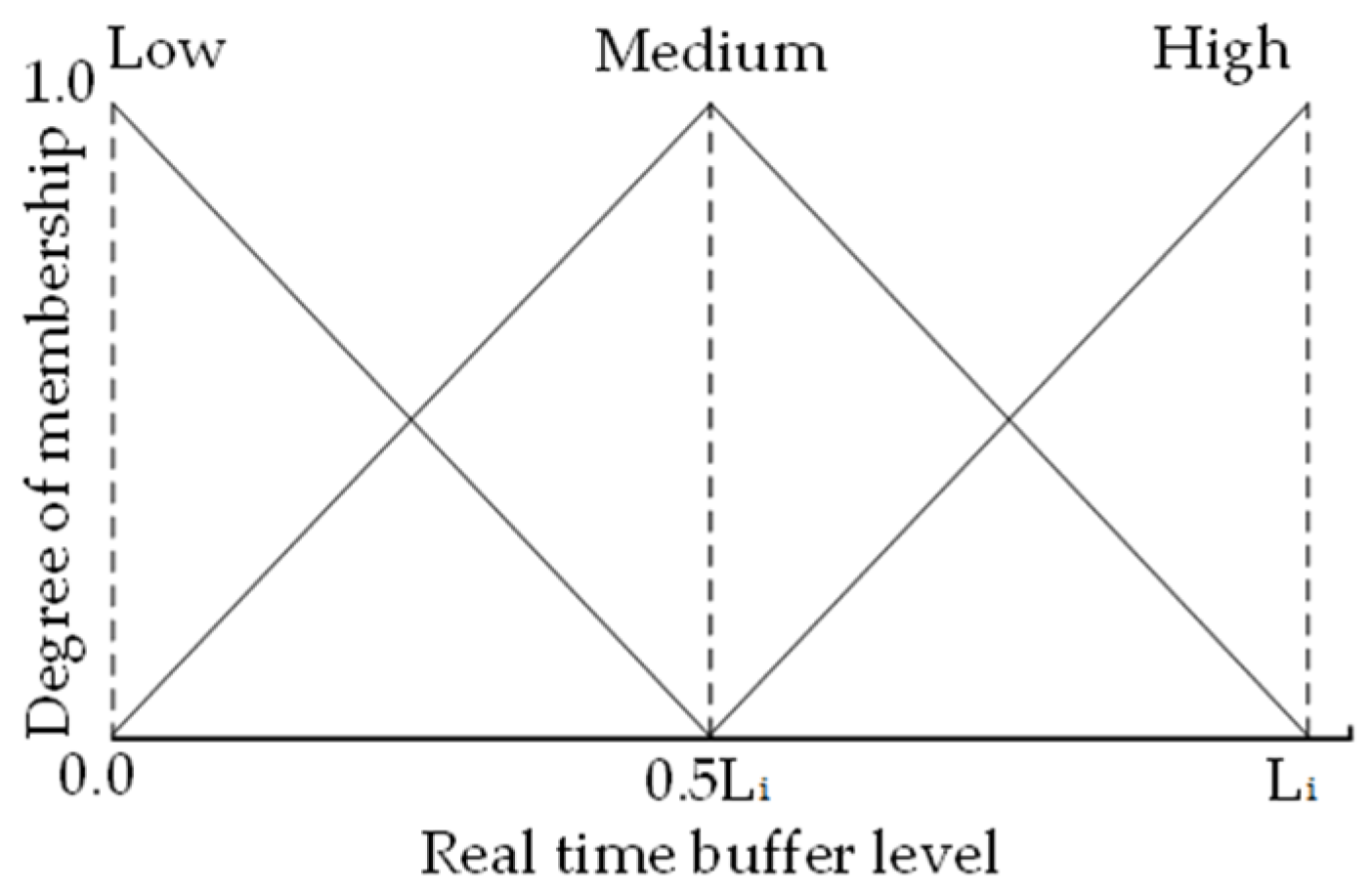
  • UB and DB are the fuzzy sets of buffer levels which are described in 3 linguistic variables {Low, Medium, High} in this paper.
  • si(t) is the decided machine state, i.e., SR = {Sleep, Running}, at time t.
  • The parameter μx = {μs, μr} defined in the universe of discourse [0,1] is the certainty factor (CF) representing the strength of the certainty of WFPRs when si(t) is {sleep} and {running} respectively.
  • wub,x and wdb,x are the set of weights, which are defined in the universe of discourse [0,1] and assigned to the first and second antecedent propositions in the rules. The weights show the relative importance of each antecedent proposition to the consequence proposition. The sum of the proposition weights equals to 1.
All the knowledge defined in WFPRs for energy saving state decisions of power-on machine are shown in Table 1 and explained as following.
Table 1. Weighted adaptive fuzzy production rules for machine state decisions.
In the antecedent propositions of the WFPRs, six abbreviations are used as {UBL, UBM, UBH, DBL, DBM, DBH} in this paper. For example, UBL means the level of the upstream buffer is low and DBM means the level of the downstream buffer is medium. Each linguistic variable has a membership function. The triangle membership function of the buffer level is adopted in Figure 2 according to [28] and the optimization of membership function is not the focus of this paper. At each decision time point, the real level of buffers is sampled and the degree of membership is calculated. Different weighted fuzzy production rules can be activated for energy saving decisions based on the PN reasoning in the next section.
Figure 2. Membership functions of a buffer level.
Each antecedent proposition has a weight, i.e., ω u b , x   and   ω d b , x , which means the relative degree of importance of a proposition contributing to the consequent proposition. For example, if the level of the upstream buffer bi(t) is sampled as {Low} and the level of downstream buffer bi+1(t) is also sampled as {Low} at a time point, the machine has a high-risk of starvation but a low-risk of blockage. For the energy saving purpose, the high-risk of starvation has a more important degree on a sleep decision comparing to a low-risk of blockage. It is reasonable to assign a larger weight to antecedent proposition {bi(t) is Low} and a smaller weight to proposition {bi+1(t) is Low} in the first rule shown in Table 1.
The CF in a WFPR indicates the degree of certainty of a rule. The larger the value of a certainty factor, the more the consequent proposition of a rule is believed. The traditional CF is a constant determined by an expert. Our objective is to sleep the machine and save more energy while not sacrificing the machine/system throughput. The decision rules should dynamically balance energy saving operations and product throughput between decision cycles. In this study, the CF is used to dynamically change the truth of a WFPR rule based on the production rate of a machine during the production. For example, when the production rate of a machine is low during a decision cycle, the sleep decision of a WFPR has small truth and the running decision has large truth in order to improve the machine/system throughput. The rules are defined to infer the CF of WFPRs in a decision cycle as follows:
R y : IF   r i ( t )   is   P R   THEN   μ s   is   C V S   AND   μ r   is   C V R ,
where ri(t) is the production rate of a machine within a decision cycle, PR is a fuzzy set, CVS and CVR are the certainty values of the sleep decision and the running decision respectively.
The ri(t) of a machine is zero when no parts are processed during a decision cycle. The maximum production rate will be 1 τ i when the machine always processes parts in a decision cycle. The production rate is calculated as follows:
r i ( t ) = T P i ( t ) T P i ( t d c ) d c
where dc is the decision cycle, TPi(t) and TPi(t-dc) is the throughput of machine i.
The PR is represented with a fuzzy term set {Low, Medium, High}. This study uses a symmetrical triangle membership function [ 0 , 1 2 τ i , 1 τ i ] for PR shown in Figure 3a. CVS and CVR take the fuzzy term set {Small, Middle, Big} with the triangle membership function [0, 0.5, 1] as shown in Figure 3b,c. The rules for CF reasoning are shown in Table 2. The Mandani scheme is used during the reasoning process of μs and μr. The knowledge of rules in Table 2 is straightforward. If the production rate of a machine is higher in a decision cycle, a bigger CF for a sleep decision and a smaller CF for a running decision will be assigned to the WFPRs aiming to compromise the energy saving behavior and the machine throughput in the next decision cycle.
Figure 3. Membership function: (a) Production rate of a machine; (b) Certainty value of sleep decision; (c) Certainty value of running decision.
Table 2. The fuzzy rules for certainty factor reasoning.

4. Dynamic Adaptive Fuzzy Reasoning Petri Net for Energy Efficient Operation

4.1. Formal Definition of Dynamic Adaptive Fuzzy Reasoning Petri Net

As a graphical and mathematical modeling tool, a Petri net is widely used to describe and study information processing systems. For a rule-based reasoning process, the graphical description of a PN can visualize the structure of a rule-based system and make the model relatively simple and legible. The algebraic equations of a PN can provide a mathematical foundation to express the dynamic behavior of a system. In this section, a dynamic adaptive fuzzy reasoning PN is proposed to implement machine state reasoning for energy saving operations in a manufacturing system for the first time.
A dynamic adaptive fuzzy reasoning Petri net (Figure 4) is built for the machine states decision based on the fuzzy knowledge (Table 1 and Table 2) and can be defined as a 9-tuple:
D A F R P N = ( P ,   T N ,   I ,   O ,   D ,   W ,   μ ,   α ,   β )
where
Figure 4. Dynamic adaptive fuzzy reasoning Petri net for machine states decision.
  • P = { p 1 , p 2 ,   ,   p m } 
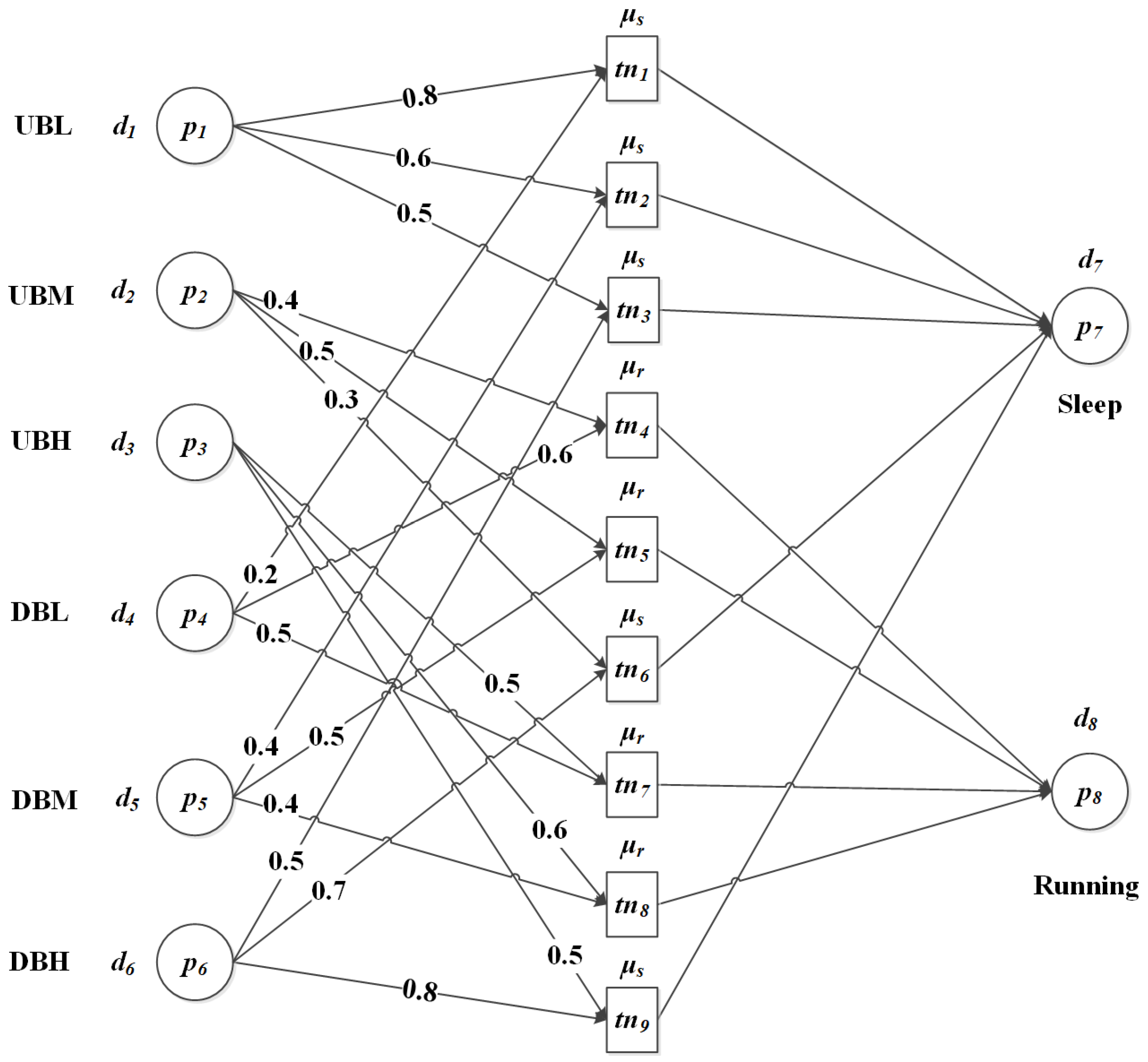
is a finite set of propositions or called places, P = P S P T , including a set of starting places P S = { p P | * p =   a n d   p * } , a set of terminating places P T = { p P ( * p   a n d   p * = } . Here, * p is the set of all input transitions of p, and p * is the set of all output transitions of p. Variable m is the number of propositions in the rules. In this paper, there are 8 places, i.e., m = 8. | P S | = 6 , which represent three linguistic levels of upstream buffers and three linguistic levels of downstream buffers. | P T | = 2 represents the two decision states {sleep, running} of a machine.
  • T N = { t n 1 , t n 2 ,   ,   t n x } is a finite set of transitions, representing a set of fuzzy inference rules. Variable x is the number of rules. In this paper, there are 9 rules and x = 9 . Transitions t n 1 t n 9 correspond to rules R 1 R 9 shown in Table 1.
  • D = { d 1 , d 2 ,   ,   d m } , a finite set of propositions in the fuzzy knowledge base. | P | = | D | . P T D = . For example, the proposition d 1 = {UBL} describes the fuzzy level of upstream and the proposition d 7 = {Sleep} is the decision result of the machine at the next decision cycle.
  • I :   P S T N , the input function, defining the directed arcs from starting places to transitions.
  • O :   T N P T , the output function, defining the directed arcs from transitions to terminating places.
  • W :   P × T N [ 0 ,   1 ] , an input function whose elements are the weights of input places, which indicates that how much an input place (or corresponding antecedent proposition) impacts on its transition. The sum of the antecedent proposition weights of a transition is equal to 1.
  • μ :   T N × P [ 0 ,   1 ] , an output function whose elements are the certainty factors of the transitions/rules, indicating how much a transition/rule impacts on its output places, i.e., the decided machine state. μ is adjusted automatically based on the changing production conditions.
  • α :   P [ 0 ,   1 ] , a correlation function, representing mapping from a set of places to a set of real values in [0,1]. α ( P i ) is the fuzzy value of a starting place, indicating the truth degree of proposition d i .
  • β :   P D , a correlation function, represents a bidirectional mapping between a set of places and a set of propositions. For example, β ( p 1 )   means   the   mapping   between   d 1   and {UBL}.

4.2. Knowledge Reasoning for Energy Saving State Decisions of A Machine

In our model, each starting place has a token. At each decision time point, the real level of the upstream and downstream buffer is collected from the manufacturing system by the IoT. The actual buffer level is converted into fuzzy linguistic values which have different fulfillment degrees, i.e., α ( p i ) , based on membership functions. Let ( t n ) = { p i } , i = 1 , 2 , 6 , O ( t n ) = { p k } ,   k = 7 , 8 , certainty factors μ ( t n ) = { μ j } ,   j = 1 , 2 , , 9 , the weights of input places are represented as w 11 , w 12 , , w i j .
• Enabling criterion
t n T N , transition tn is enabled for p i I ( t n ) ,
α ( p i ) > 0 ,
• Firing criterion
When tn is fired, a token in the starting place is copied and a token with an equivalent truth value is put into the output place.
If | * p | = 1 , the output place has only one input transition. The equivalent fuzzy value of an output place is defined by:
α ( p k ) = μ j × [ α ( p i ) × w i j ] ,   k = 7 , 8
If | * p | > 1 , the output place has more than one input transition. The equivalent fuzzy value of an output place is determined by the input transition with the maximum equivalent fuzzy value as follows:
α ( p k ) = m a x { μ j × [ α ( p i ) × w i j ] } ,   k = 7 , 8
The reasoning process of machine states can be realized in a parallel way by matrix equation as in [38] and is not described here.
• Decision Making
After the firing of all transitions, the conclusion proposition with the larger fuzzy truth value is chosen as the decided machine state at a current decision time point. During the production process, the fuzzy reasoning process based on DAFRPN will execute at each decision time point. The machine state will be switched to running or sleep, and the idle period of a machine can be reduced to achieve energy saving operations.

5. Numerical Experiments and Discussions

5.1. A Serial Automotive Powertrain Line
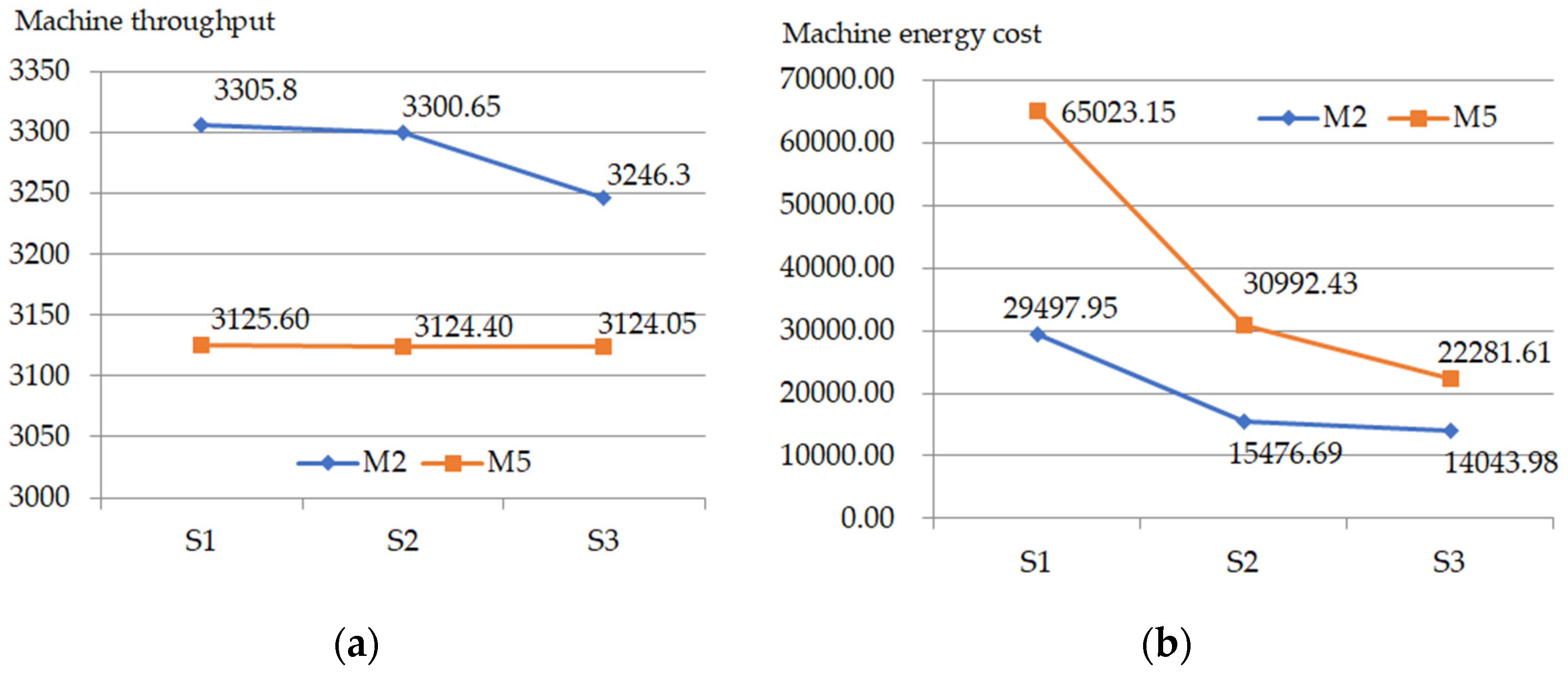
In order to illustrate the feasibility and effectiveness of our proposed method, a 6M5B serial manufacturing system is taken as a case study for comparison with the control method in [22,29]. This system is a simplified version of a real automotive powertrain production line and parameters are mocked up for confidence. The reliability models of machines are assumed as exponential distribution. The power rate is assumed to be 0.2 $/kWh. The simulation is repeated twenty times and all simulations last three weeks (30240 minutes). Table 3 and Table 4 show the system parameters.
Table 3. Parameters of machines in a serial manufacturing system.
Table 4. Parameters of buffers in a serial manufacturing system.
This study conducted simulation experiments in three scenarios: Baseline without machine control (S1); only one machine is controlled (S2), e.g., M2 or M5; multi-machines are controlled (S3), i.e., M1, M2, M3, M5, except the bottleneck machine and the last machine for maximizing the system throughput. First, the baseline scenario is simulated and the system bottleneck is identified as M4 based on the machine blockage and starvation data using the method in [39]. The decision cycle of each machine in controlled scenarios S2 and S3 is set as five times as much as its cycle time. The system performances of three scenarios are compared in Table 5.
Table 5. Comparison of system performances in three scenarios.
From Table 5, the machines have notable sleep time in S2 and S3. For single machine control, the sleep time of M2 (14021.62 min) and M5 (15468.38 min) is about 46.37% and 51.15% of their total work time (30240 min). When multi-machines are controlled simultaneously, the total sleep time of M1, M2, M3, M5 (73722.71 min) is 60.95% of the four controlled machines’ work time. The system throughput has negligible loss in all control scenarios with distinct energy cost savings. Compared with energy cost in S1, the system energy cost reduces by 6.21%, 15.07%, 45.18% in S2(M2), S2(M5) and S3 when different machines are controlled. Regarding the energy cost per part, all controlled scenarios also have observable cost savings. The energy cost per part decreases from 71.24 $ in S1 to 39.08 $ in S3, which has a 45.14% cost reduction. The results show that the controlled scenarios are effective energy saving operations of the manufacturing system.

5.2. Discussions

The purpose of machine control is to sleep the machine when it has the tendency for starvation or blockage without sacrificing the machine and system throughput. The performances of M2 and M5 are shown in Figure 5 for the three scenarios. The throughput of M2 only slightly reduces approximately by 0.16% and 1.8% in S2 and S3. The energy cost of M2 dramatically reduces from 29497.95 (S1) to 15476.69 (S2) and 14043.98 (S3), which save 47.53% and 52.39% of the energy cost respectively. The M5 has negligible throughput loss, i.e., 0.04% and 0.05% of S1, in controlled scenarios, which means the control method does not affect the productivity of M5. The machine M5 achieves a 52.34% energy cost reduction in S2 and a 65.73% energy cost reduction in S3 compared with S1. From the single machine aspect, the control method has a remarkable effect for energy saving operations.
Figure 5. The performances of machine M2 and M5 in three scenarios: (a) Throughput of machines; (b) Energy cost of machines.
Table 6 shows the time length of different states, which are throughput loss (TPL) and energy cost reduction (ECR) of each machine in S1 and S3. It can be seen that the processing time of each machine in S3 has a slight reduction compared with S1, which results in a corresponding loss of the machine throughput. When multi-machines are controlled, the blockage and starvation time of machines are obviously decreased and are changed into sleep time. In S1, the total idle time of M3 is 20997.81 minutes. In S3, machine M3 has the longest sleep time, i.e., 20676.43 minutes, which reaches 98.47% conversion of the idle time and accounts for 68.37% of the total simulation time. Among the controlled machines, M1 has the largest throughput loss percentage (2.29%) in S3. The throughput of bottleneck M4 statistically keeps the same, which indicates the multi-machine control has no influence on the bottleneck machine M4. Each controlled machine has gained over 50% of energy cost savings, with only 0.06% system throughput loss.
Table 6. Time length of machine states and machine performances comparison in S1 and S3.
During the simulation, this study recorded the main parameters at each decision time point. Figure 6 is a randomly sampled experiment time phase in S3 from 22512 minutes to 24591 minutes, which shows the state changing, the production rate and the level of related buffers for M2.
Figure 6. A random sampled simulation in S3 at each decision time point: (a) Level of buffer before/after M2; (b) Processing rate of M2; (c) State change of M2.
From Figure 6a, it can be concluded that the buffer, B1 and B2, are not empty or full when multi-machines are controlled in S3. Consequently, the blockage/starvation time of M1, M2 and M3 are greatly decreased as shown in Table 6. Due to the sleep and failure times, the production rate of M2 is changed accordingly in Figure 6b. Based on the buffer level and production rate, the state of M2 is decided using the DAFRPN. For example, at time point 23142, the machine is still at the failure state with zero production rate and buffer level {b1 = 115, b2 = 98}. Twenty-one minutes later, i.e., 23163 minutes, the production rate is 0.0930 and the buffer level is b1 = 112, b2 = 102. The decided state of M2 is running, as shown in Figure 6c. The machine continually processes parts until the next decision time point, 23184. The production rate is 0.2093 and the buffer level is b1 = 110, b2 = 107. The state of M2 will be switched as sleep based on the DAFRPN. After two decision intervals, i.e., 23226 minutes, the machine will be woken up with the production rate 0.0233 and buffer level {b1 = 110, b2 = 108}. It reveals that M2 is turned into a sleep state if it has the tendency of blockage or starvation with higher production rates.
In order to investigate the performance of our dynamic adaptive fuzzy reasoning Petri net method, the results of the mathematical method of energy saving opportunity windows [22] and the fuzzy control method [29] for the above case line are compared in Table 7. Our method has the least throughput loss when a single machine and multi-machines are controlled. The energy cost reduction in S3 of our method is higher than [22] but lower than [29]. Compared with the fuzzy control method in [29], our method has less parameters to be set for control. There are many threshold values that must be adjusted for better control performance [29], which is time consuming and not practical in actual application. The mathematical method in [22] assumed that there was a slow machine in the line which meant their method is only applicable to asynchronous lines. Our method has no restriction on machine cycle time and can be used for both synchronous and asynchronous manufacturing systems. If it is assumed the profit per part produced is 300 $ and 600 $ respectively as in [22], the profit increase percentage of different methods considering throughput loss and energy cost can be calculated (Table 7). It is obvious that the increase percentage of a system profit will decrease owing to the reduced throughput with higher prices for parts. As the method in this study has the least throughput loss, it can be seen that the profit increase percentage of this method has less reduction when produced parts are more valuable.
Table 7. System performance comparison of different methods.
The system performances of different decision cycles in S3 are compared in Table 8 with the same WFPR weights. Decision cycles are set as two times, five times and ten times as much as the machine cycle time respectively. From Table 8, it can be found that the system throughput do not have an obvious change under different decision cycles. When a longer decision cycle is adopted, the total sleep time gets smaller, and the total energy cost and the energy cost per part becomes larger. A longer decision interval means a less frequent data collection from the workshop, which makes it harder to catch the transient state of the system, thus missing some energy saving chances to reduce idle time. A smaller decision interval can catch much more energy saving opportunities but with a frequent switch between a sleep state and processing state. Based on the cycle time of machines and the results of simulation experiments, an appropriate decision cycle interval should be determined.
Table 8. System performance comparison of different decision cycles in S3.
The selection of different input weight combinations will influence the effects of the energy saving method. Many groups of input weights have been adopted in our simulation experiments, from which three groups chosen as examples (G1, G2, G3) and the system performances of these three groups are shown in Table 9. The decision cycle is five times as much as the cycle time in these three experiments. It can be seen that different input weight groups all obtain the energy cost reduction and have certain effects on system performances. The optimal combination of input weights can be determined based on the results of simulation experiments and the actual situation of the shop floor in the future work.
Table 9. System performance comparison of input weights group in S3.
In this paper, the authors do not consider the warm-up energy from a sleep state to a running state in order to compare the results with the literature [22,29]. The proposed method can be used when a warm-up process is taken into account. In our method, the elements of the DAFRPN, such as the amount of places and arcs, can be varied if the granularity of the buffer level in linguistic values and the number of decided machine states are changed. For example, the buffer level can be described in five grads {Very low, Low, Medium, High, Very high} and the machine can have three decided states {Light sleep, Deep sleep, Running}. The DAFRPN can be adjusted conveniently based on the newly defined WFPRs of the energy saving operation knowledge, which will have twenty-five rules. There will be ten starting places and three terminating places in the DAFRPN. This makes the DAFRPN method more flexible for different control granularity.

6. Conclusions

Energy saving operations of manufacturing systems is a popular research topic in academia and industry for sustainable development. Due to the stochastic and dynamic properties of manufacturing systems, the real-time energy saving operations considering production conditions is a difficult problem at a system level. A control method based on dynamic adaptive fuzzy reasoning Petri nets is proposed to make a decision on machine states for reducing idle times. Weighted fuzzy production rules with certain values are used to describe fuzzy knowledge of machine state decisions considering online production information. The real-time production rate and buffer levels are formatted as linguistic fuzzy sets to represent the imprecise knowledge of machine operations. The fuzzy knowledge describes the purpose for energy saving operation, i.e., turning the machine to sleep if the machine has an inclination of starvation or blockage during the production process. A dynamic adaptive fuzzy reasoning Petri net is formally defined in this paper to implement reasoning processes of machine state decisions. A serial automotive powertrain line is taken to conduct simulation experiments. The results of three scenarios show the effectiveness and flexibility of our method for energy saving manufacturing system operations. For future works, the energy saving operation method based on dynamic adaptive fuzzy reasoning Petri nets will be extended and applied to manufacturing systems with parallel, assembly or disassembly structures.

Author Contributions

The authors contributed equally to this work.

Funding

This research was funded by National Natural Science Foundation of China grant number No. 71571075.

Acknowledgments

Authors thank the anonymous reviewers for the valuable comments.

Conflicts of Interest

The authors declare no conflicts of interest.

Abbreviations and Nomenclature

AbbreviationsDescription
PNsPetri nets
FRPNsFuzzy reasoning Petri nets
FPRsFuzzy production rules
WFPRsWeighed fuzzy production rules
DAFRPNDynamic adaptive fuzzy reasoning Petri net
PSProcessing state
STStarvation state
BLBlockage state
FLFailure state
SLSleep state
CFCertainty factor
UBLThe level of the upstream buffer is low
DBMThe level of the downstream buffer is medium
CIConfidence interval
TPLThroughput loss
ECREnergy cost reduction
P S Starting places
P T Terminating places
τ i Cycle time of Mi,
LiBuffer capacity of Bi
bi(t)Buffer level of Bi at time t
Eps,iEnergy consumption of processing state
Eid,iEnergy consumption of idle state
Esl,iEnergy consumption of sleep state
Tps,iTime length of processing state
Tid,iTime length of idle state
Tsl,iTime length of sleep state
E i ( T ) Energy consumption of Mi in time (0,T]
E s y s ( T ) Energy consumption of the system during time (0,T]
bi(t)Level of the upstream buffer of Mi at time point t
bi+1(t)Level of the downstream buffer of Mi at time point t
si(t)Decided machine state
μsCertainty factor of WFPR when si(t) is sleep
μrCertainty factor of WFPR when si(t) is running
wub,xWeight of the first antecedent proposition in the rule
wdb,xWeight of the second antecedent proposition in the rule
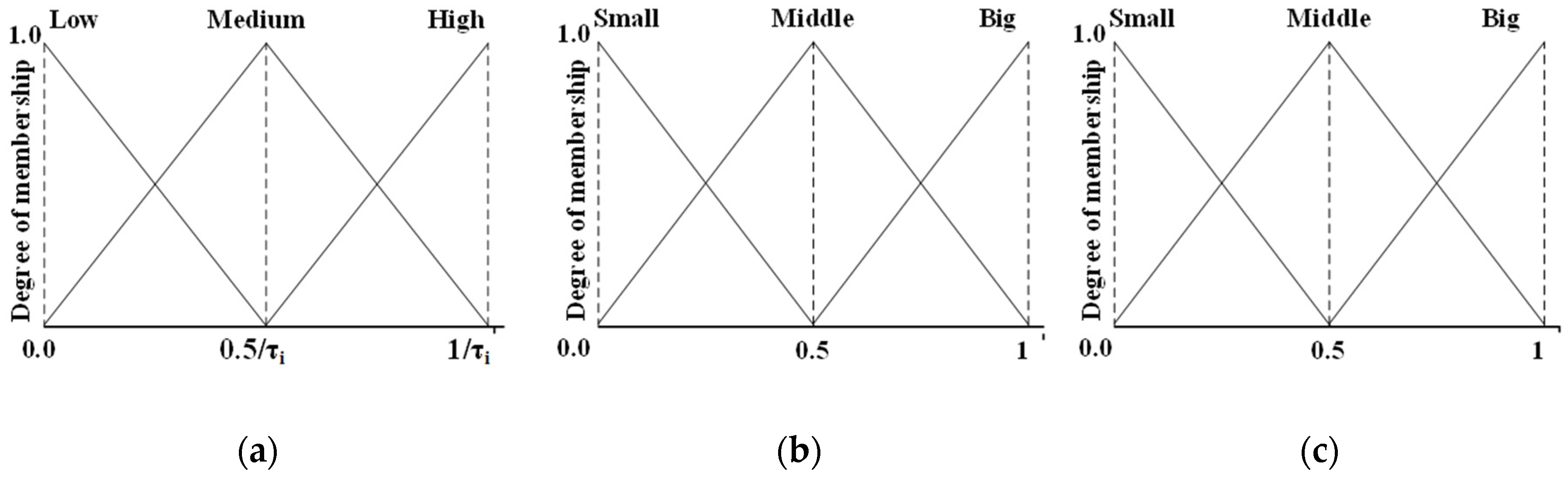
ri(t)Production rate of Mi within decision cycle
dcDecision cycle
TPi(t)Throughput of Mi at time point t

References

  1. Park, C.W.; Kwon, K.S.; Kim, W.B.; Min, B.K.; Park, S.J.; Sung, I.H.; Seok, J. Energy consumption reduction technology in manufacturing–a selective review of policies, standards, and research. Int. J. Precis. Eng. Manuf. 2009, 10, 151–173. [Google Scholar] [CrossRef]
  2. Energy Information Administration. Available online: http://www.eia.gov/outlooks/aeo/pdf/0383(2015).pdf (accessed on 20 December 2016).
  3. Zhang, X.P.; Cheng, X.M. Energy consumption, carbon emissions, and economic growth in China. Ecol. Econ. 2009, 68, 2706–2712. [Google Scholar] [CrossRef]
  4. Thomas, Z.; Charlotte, M. Evaluating the management system approach for industrial energy efficiency improvements. Energies 2016, 9, 774. [Google Scholar]
  5. Lawrence, A.; Thollander, P.; Andrei, M.; Karlsson, M. Specific energy consumption/use (SEC) in energy management for improving energy efficiency in industry: Meaning, usage and differences. Energies 2019, 12, 247. [Google Scholar] [CrossRef]
  6. International Energy Agency. Available online: http://indiaenvironmentportal.org.in/files/Indicators_2008.pdf (accessed on 20 October 2008).
  7. Gutowski, T.G.; Allwood, J.M.; Herrmann, C.; Sahni, S. A global assessment of manufacturing: Economic development, energy use, carbon emissions, and the potential for energy efficiency and materials recycling. Annu. Rev. Environ. Resour. 2013, 38, 81–106. [Google Scholar] [CrossRef]
  8. Patrik, T.; Jenny, P. Industrial energy management decision making for improved energy efficiency—strategic system perspectives and situated action in combination. Energies 2015, 8, 5694–5703. [Google Scholar]
  9. Twomey, J.; Yildirim, M.; Whitman, B.L.; Liao, H.; Ahmad, J. Energy Profiles of Manufacturing Equipment for Reducing Energy Consumption in A Production Setting. Working Paper; Wichita State University: Wichita, KS, USA, 2008. [Google Scholar]
  10. Peng, C.; Peng, T.; Zhang, Y.; Tang, R.; Hu, L. Minimising non-processing energy consumption and tardiness fines in a mixed-flow shop. Energies 2018, 11, 3382. [Google Scholar] [CrossRef]
  11. Mouzon, G.; Yildirim, M.B.; Twomey, J. Operational methods for minimization of energy consumption of manufacturing equipment. Int. J. Prod. Res. 2007, 45, 4247–4271. [Google Scholar] [CrossRef]
  12. Prabhu, V.V.; Jeon, H.W.; Taisch, M. Modeling green factory physics-an analytical approach. In Proceedings of the 8th IEEE International Conference on Automation Science and Engineering, Seoul, Korea, 20–24 August 2012. [Google Scholar]
  13. Mashaei, M.; Lennartson, B. Energy reduction in a pallet-constrained flow shop through on–off control of idle machines. IEEE Trans. Autom. Sci. Eng. 2013, 10, 45–56. [Google Scholar] [CrossRef]
  14. Frigerio, N.; Matta, A. Energy-efficient control strategies for machine tools with stochastic arrivals. IEEE Trans. Autom. Sci. Eng. 2015, 12, 50–61. [Google Scholar] [CrossRef]
  15. Jia, Z.; Zhang, L.; Arinez, J.; Xiao, G. Performance analysis for serial production lines with Bernoulli machines and real-time WIP-based machine switch-on/off control. Int. J. Prod. Res. 2016, 54, 1–17. [Google Scholar] [CrossRef]
  16. Chang, Q.; Xiao, G.; Biller, S.; Li, L. Energy saving opportunity analysis of automotive serial production systems. IEEE Trans. Autom. Sci. Eng. 2013, 10, 334–342. [Google Scholar] [CrossRef]
  17. Sun, Z.; Li, L. Opportunity estimation for real time energy control of sustainable manufacturing systems. IEEE Trans. Autom. Sci. Eng. 2013, 10, 38–44. [Google Scholar] [CrossRef]
  18. Li, L.; Sun, Z. Dynamic energy control for energy efficiency improvement of sustainable manufacturing systems using Markov decision process. IEEE Trans. Syst. Man Cybern. Syst. 2013, 43, 1195–1205. [Google Scholar] [CrossRef]
  19. Li, Y.; Chang, Q.; Ni, J.; Brundage, M.P. Event-based supervisory control for energy efficient manufacturing systems. IEEE Trans. Autom. Sci. Eng. 2018, 15, 92–103. [Google Scholar] [CrossRef]
  20. Li, Y.; Wang, J.; Chang, Q. Event-based production control for energy efficiency improvement in sustainable multistage manufacturing systems. ASME J. Manuf. Sci. Eng. 2018, 141. [Google Scholar] [CrossRef]
  21. Zou, J.; Arinez, J.; Chang, Q.; Lei, Y. Opportunity window for energy saving and maintenance in stochastic production systems. Trans. ASME J. Manuf. Sci. Eng. 2016, 138, 121009. [Google Scholar] [CrossRef]
  22. Zou, J.; Chang, Q.; Arinez, J.; Xiao, G.X. Data-driven modeling and real-time distributed control for energy efficient manufacturing systems. Energy 2017, 127, 247–257. [Google Scholar] [CrossRef]
  23. Hibino, H.; Yanaga, K. Decision support for energy-saving idle production facility operations in a production line based on an M2M environment. Procedia CIRP 2017, 61, 399–403. [Google Scholar] [CrossRef]
  24. Azadegan, A.; Porobic, L.; Ghazinoory, S.; Samouei, P.; Kheirkhah, A.S. Fuzzy logic in manufacturing: A review of literature and a specialized application. Int. J. Prod. Econ. 2011, 132, 258–270. [Google Scholar] [CrossRef]
  25. Tsourveloudis, N.C.; Doitsidis, L.; Ioannidis, S. Work-in-process scheduling by evolutionary tuned fuzzy controllers. Int. J. Adv. Manuf. Technol. 2007, 34, 748–761. [Google Scholar] [CrossRef]
  26. Tamani, K.; Boukezzoula, R.; Habchi, G. Application of a continuous supervisory fuzzy control on a discrete scheduling of manufacturing systems. Eng. Appl. Artif. Intell. 2011, 24, 1162–1173. [Google Scholar] [CrossRef][Green Version]
  27. Precup, R.E.; Hellendoorn, H. A survey on industrial applications of fuzzy control. Comput. Ind. 2011, 62, 213–226. [Google Scholar] [CrossRef]
  28. Wang, J.; Fei, Z.; Chang, Q.; Li, S.; Fu, Y. Multi-state decision of unreliable machines for energy-efficient production considering work-in-process inventory. Int. J. Adv. Manuf. Technol. 2019, 102, 1009–1021. [Google Scholar] [CrossRef]
  29. Wang, J.; Fei, Z.; Chang, Q.; Fu, Y.; Li, S. Energy saving operation of multi-stage stochastic manufacturing systems based on fuzzy logic. Int. J. Simul. Model. 2019, 18, 138–149. [Google Scholar] [CrossRef]
  30. Liu, H.C.; You, J.X.; Li, Z.W.; Tian, G. Fuzzy petri nets for knowledge representation and reasoning: A literature review. Eng. Appl. Artif. Intell. 2017, 60, 45–56. [Google Scholar] [CrossRef]
  31. Xie, N.; Duan, M.; Chinnam, R.B.; Li, A.; Xue, W. An energy modeling and evaluation approach for machine tools using generalized stochastic petri nets. J. Clean. Prod. 2016, 113, 523–531. [Google Scholar] [CrossRef]
  32. Pang, C.K.; Le, C.V. Optimization of total energy consumption in flexible manufacturing systems using weighted p-timed petri nets and dynamic programming. IEEE Trans. Autom. Sci. Eng. 2014, 11, 1083–1096. [Google Scholar] [CrossRef]
  33. Wang, Q.; Wang, X.; Yang, S. Energy modeling and simulation of flexible manufacturing system based on colored timed Petri net. J. Ind. Ecol. 2014, 18, 558–566. [Google Scholar] [CrossRef]
  34. Li, Y.; He, Y.; Wang, Y.; Wang, Y.; Yan, P.; Lin, S. A modeling method for hybrid energy behaviors in flexible machining systems. Energy 2015, 86, 164–174. [Google Scholar] [CrossRef]
  35. Fei, Z.; Li, S.; Chang, Q.; Wang, J.; Huang, Y. Fuzzy petri net based intelligent machine operation of energy efficient manufacturing system. In Proceedings of the 14th IEEE Conference on Automation Science and Engineering (CASE), Munich, Germany, 20–24 August 2018; pp. 1593–1598. [Google Scholar]
  36. Gao, M.; Zhou, M.C.; Huang, X.; Wu, Z. Fuzzy reasoning Petri nets. IEEE Trans. Syst. Man Cybern. A 2013, 33, 314–323. [Google Scholar]
  37. Yeung, D.S.; Tsang, E.C.C. Weighted fuzzy production rules. Fuzzy Sets Syst. 1997, 88, 299–313. [Google Scholar] [CrossRef]
  38. Liu, H.C.; Lin, Q.L.; Mao, L.X.; Zhang, Z.Y. Dynamic adaptive fuzzy petri nets for knowledge representation and reasoning. IEEE Trans. Syst. Man Cybern. S 2013, 43, 1399–1410. [Google Scholar] [CrossRef]
  39. Li, J.; Meerkov, S.M.; Zhang, L. Production systems engineering: Problems, solutions, and applications. Annu. Rev. Control. 2010, 34, 73–88. [Google Scholar] [CrossRef]

Article Metrics

Citations

Article Access Statistics

Multiple requests from the same IP address are counted as one view.