Numerical Simulations and Empirical Data for the Evaluation of Daylight Factors in Existing Buildings in Sweden


Abstract
1. Introduction
1.1. Daylighting Indicators and Calculation Techniques in Use
1.2. Daylight Availability in Existing Buildings
1.3. The Layout of the Paper
2. Research Methodology
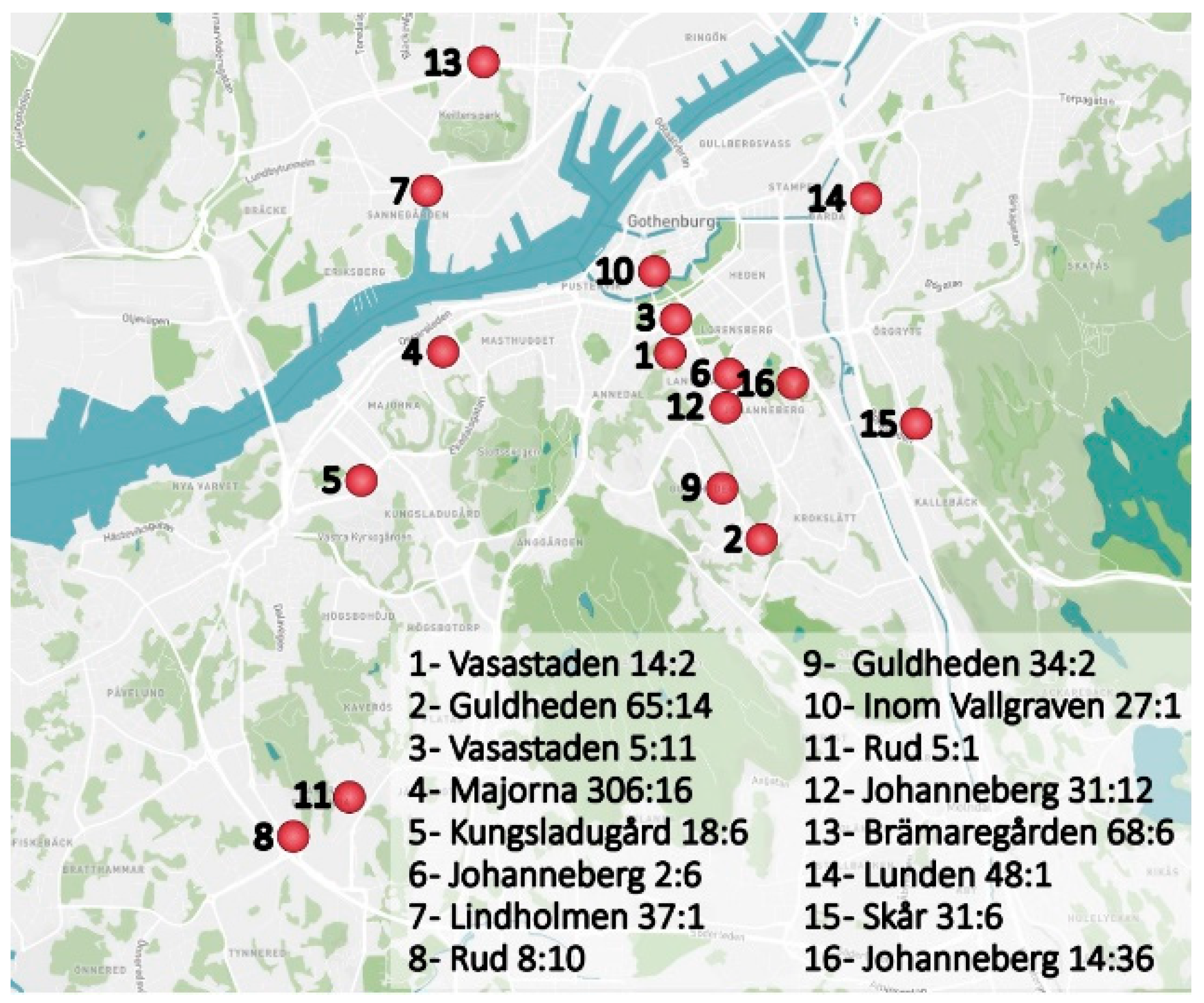
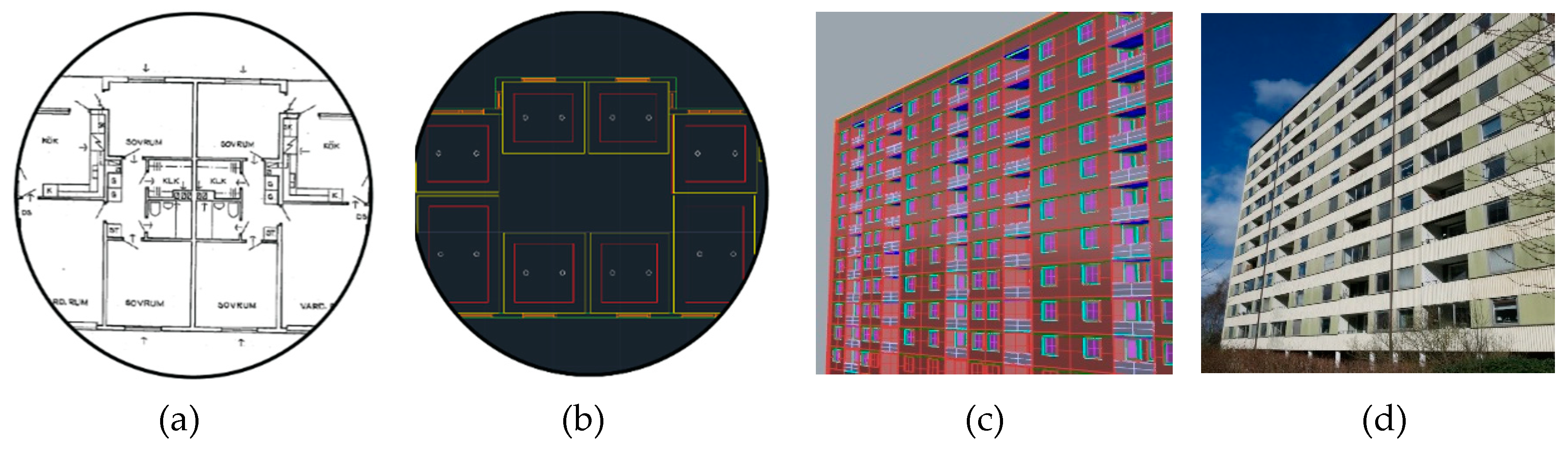
2.1. Sample Buildings and Their CAD Replicas
2.2. Optical Properties of Surfaces
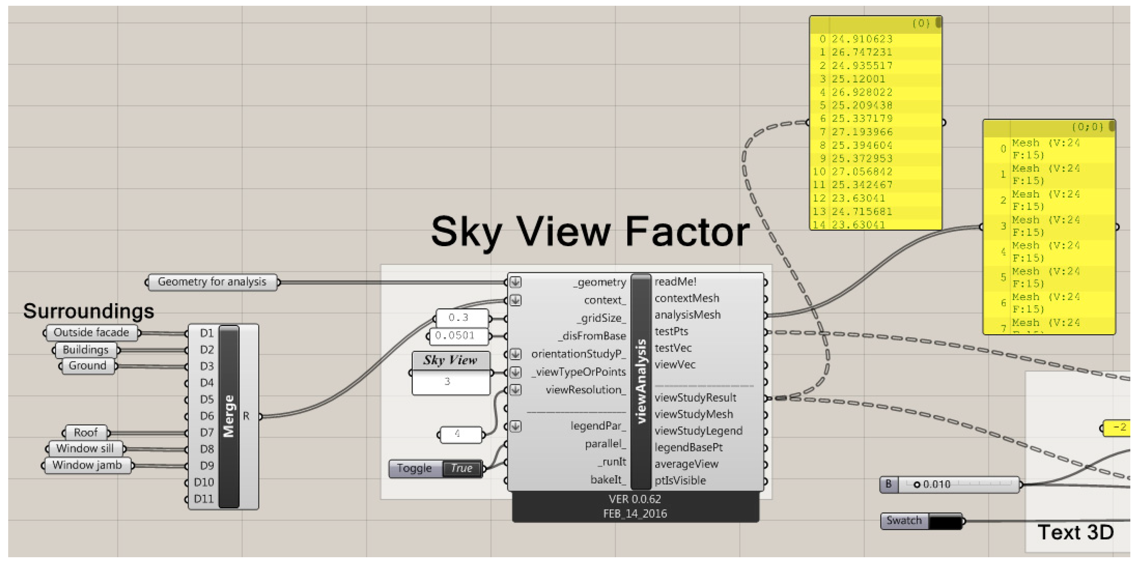
2.3. Calculation of Indoor and Outdoor Illuminance
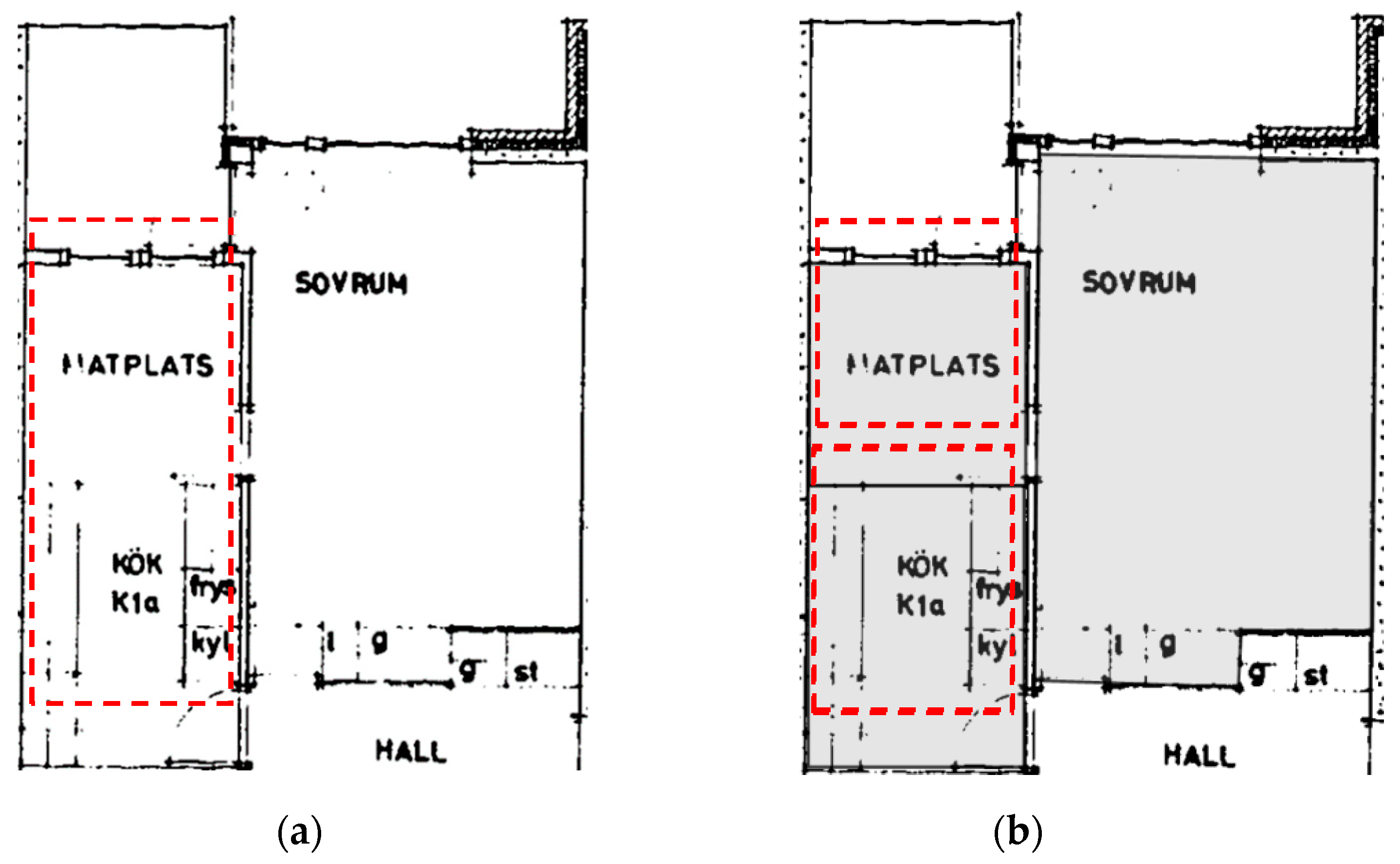
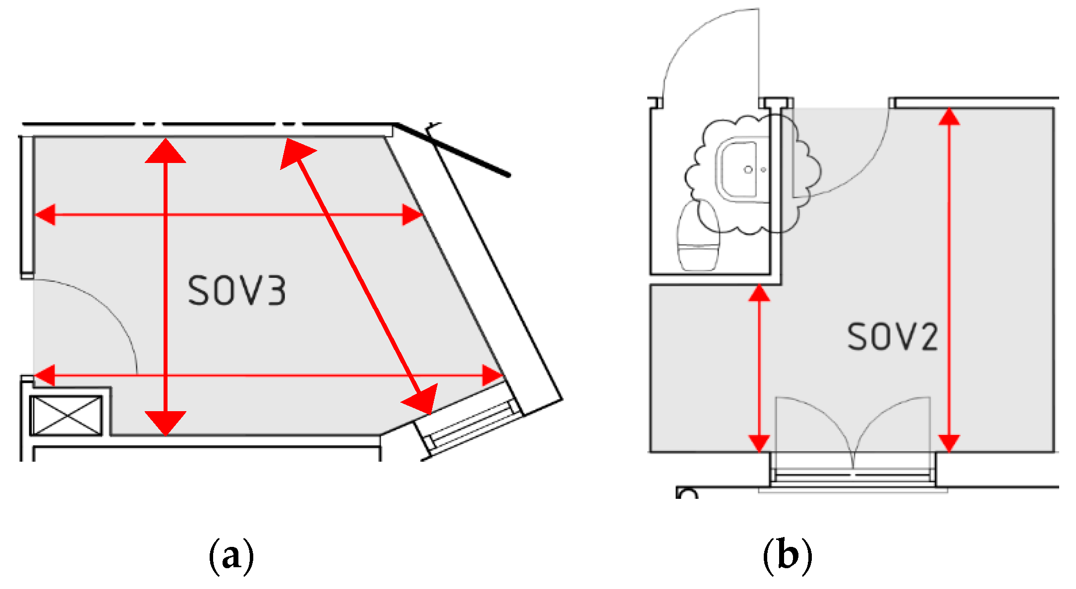
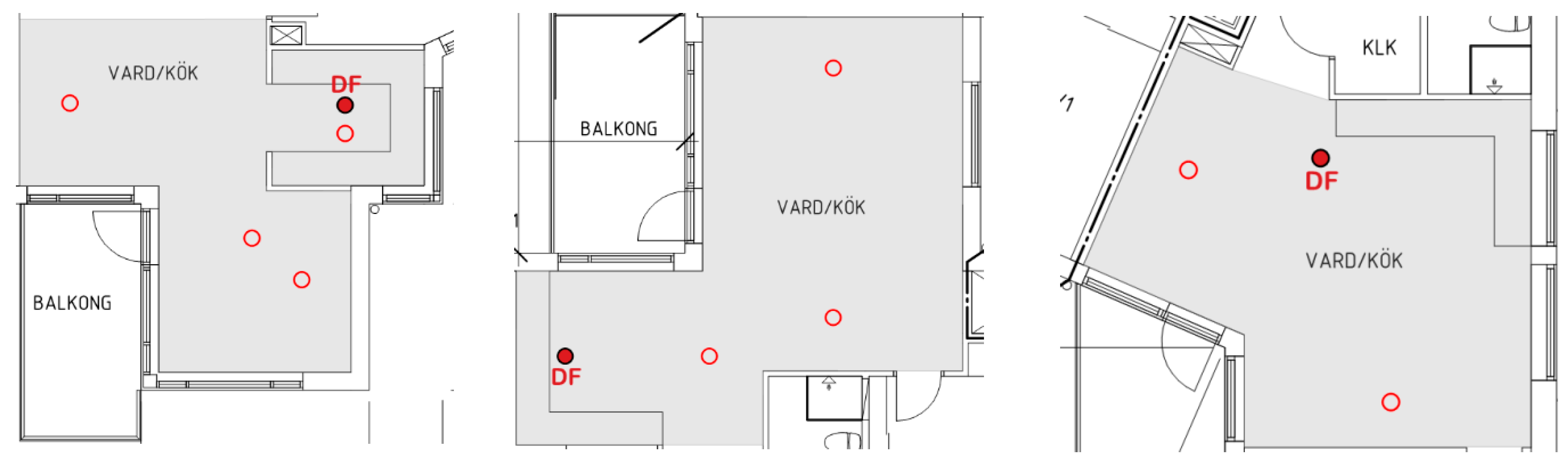
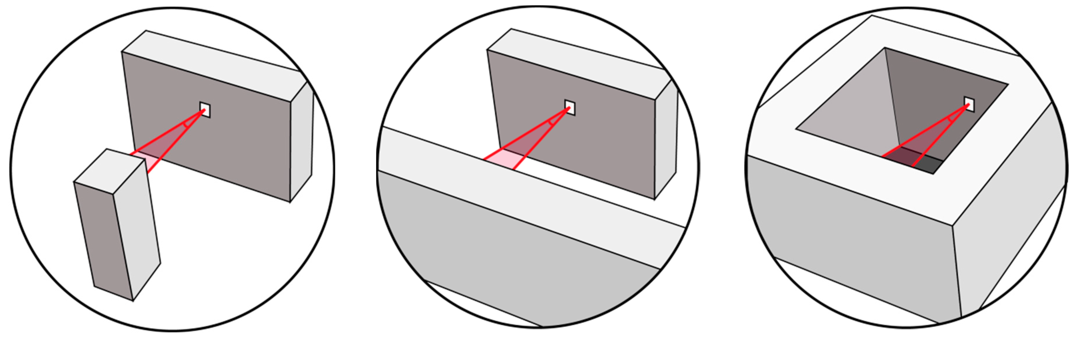
2.4. Control Points for DFP in Complex Rooms
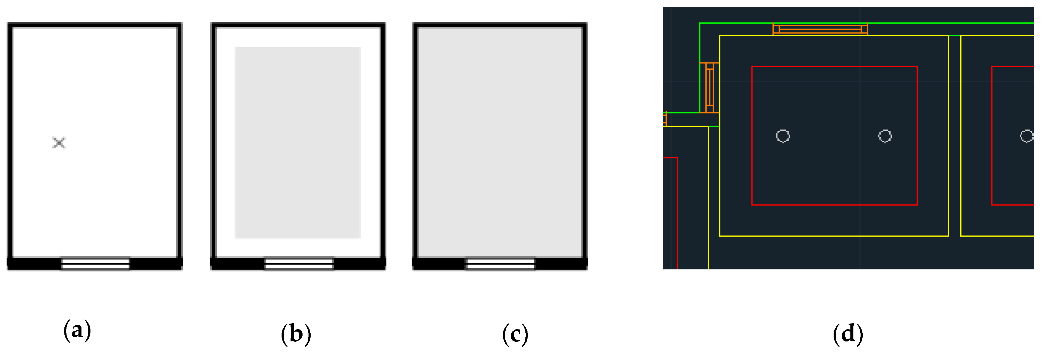
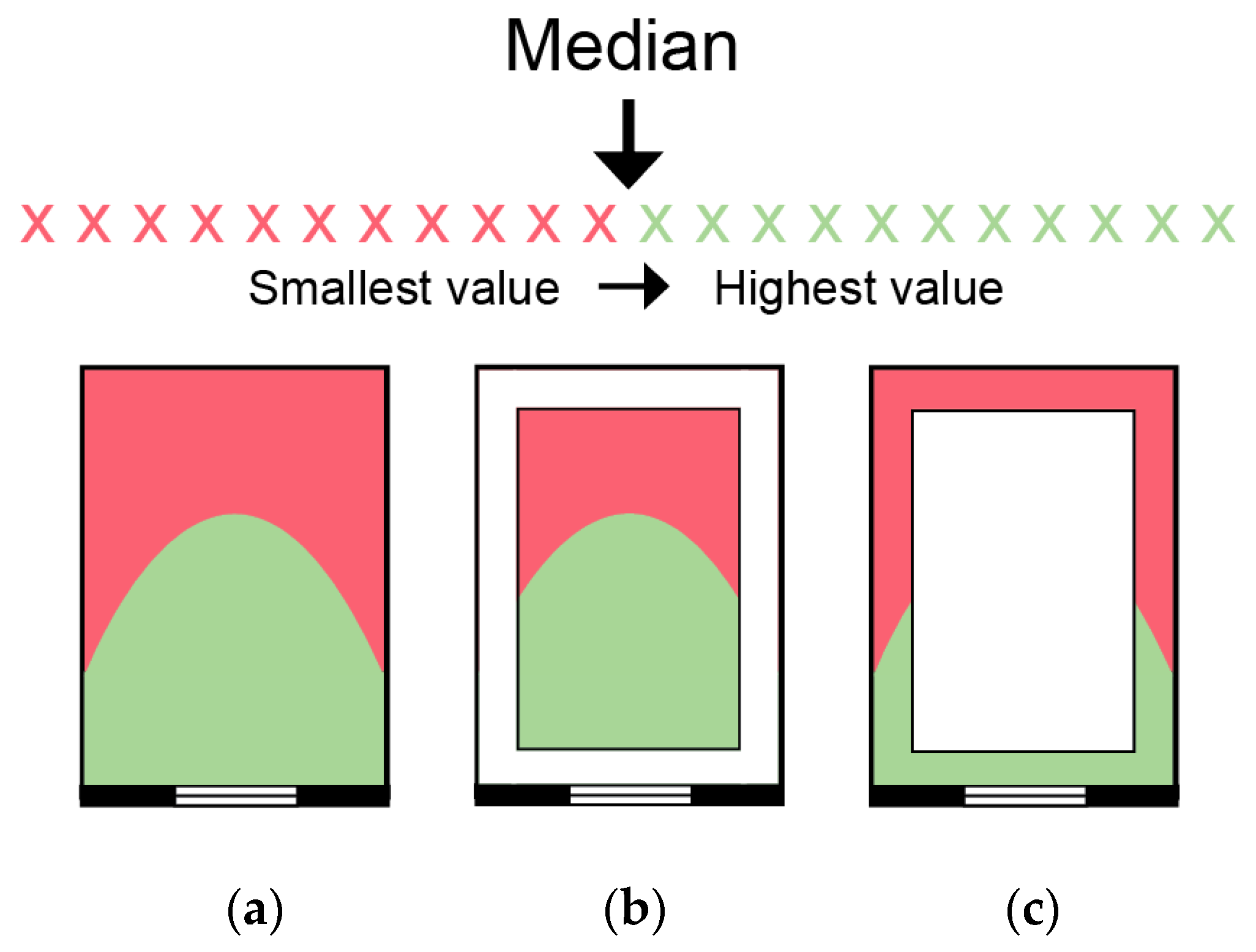
2.5. Control Surfaces and Grids for Area-Averaged DF
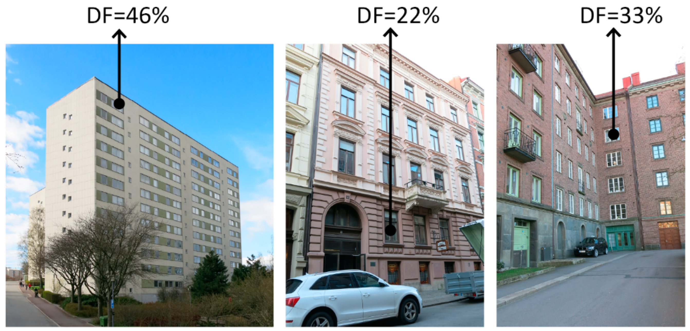
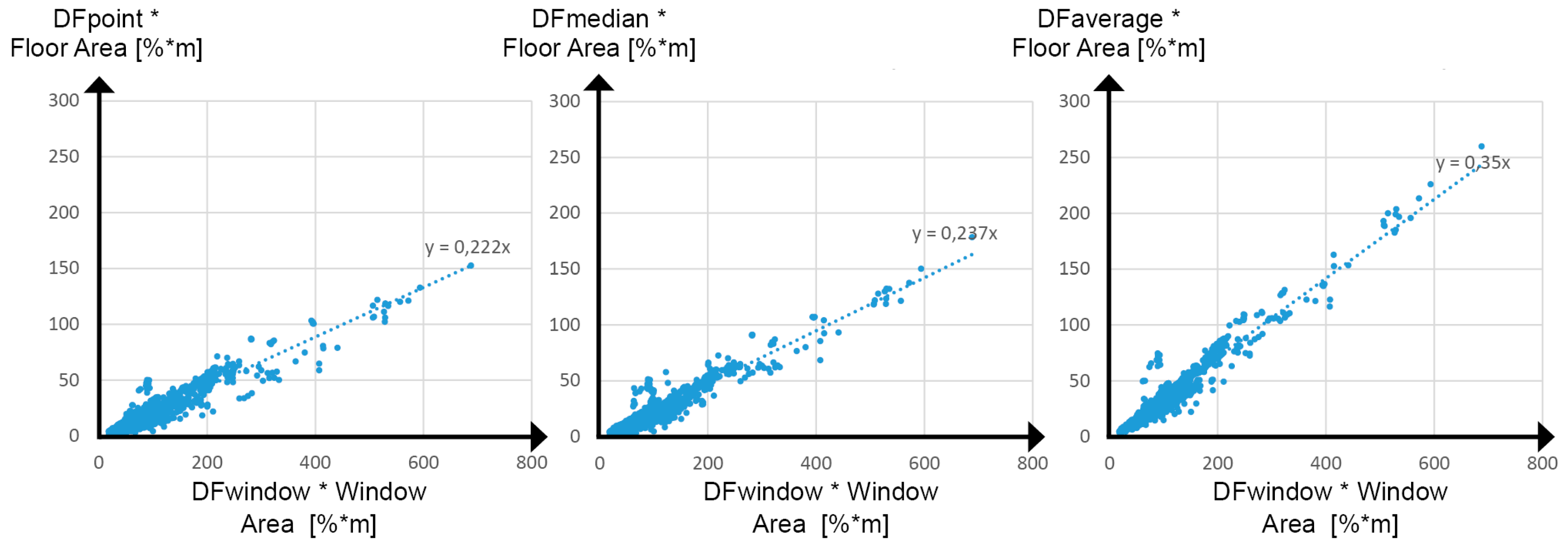
2.6. New Daylight Metrics: DFW
2.7. Field Surveys
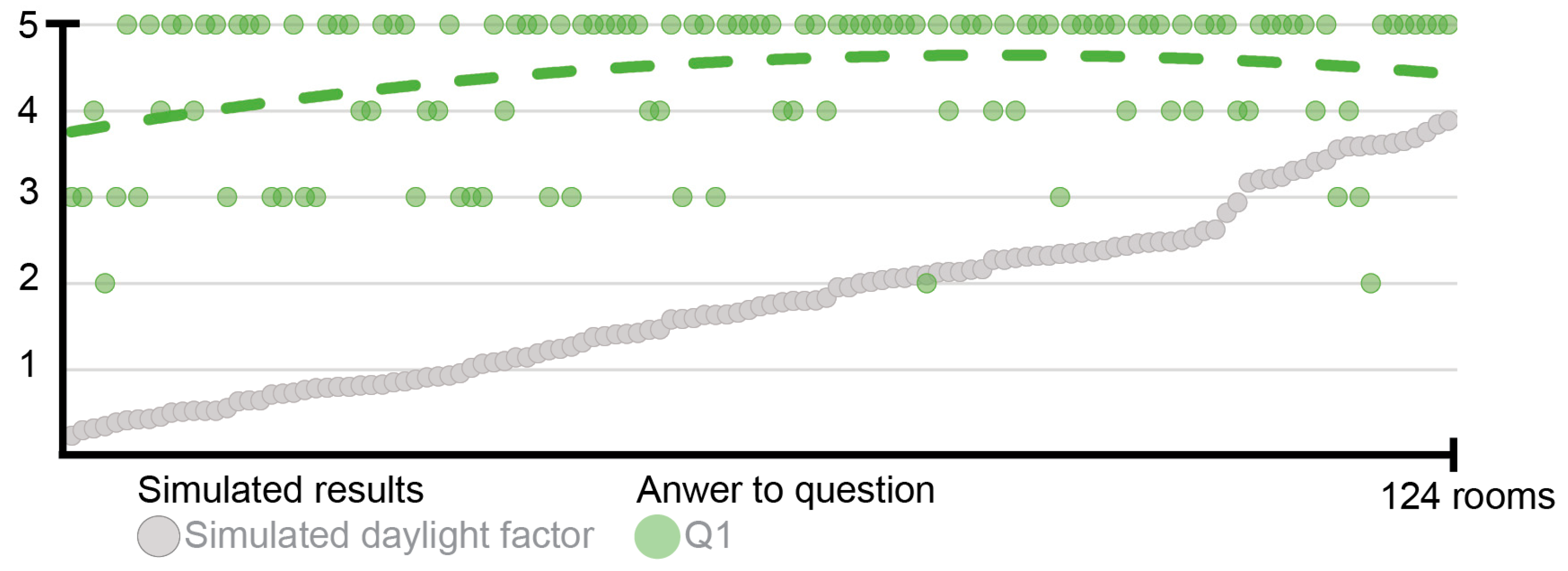
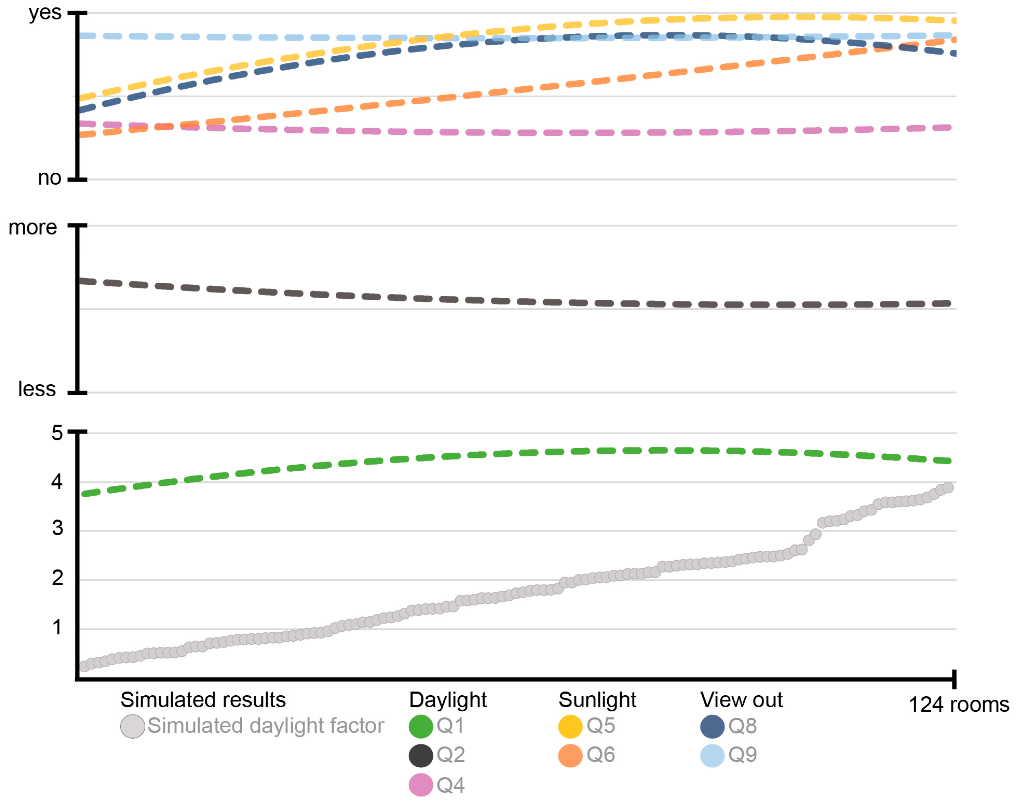
- Q1.
- How do you perceive the access to daylight in the following rooms?
- Q2.
- Would you prefer more or less daylight in these following rooms?
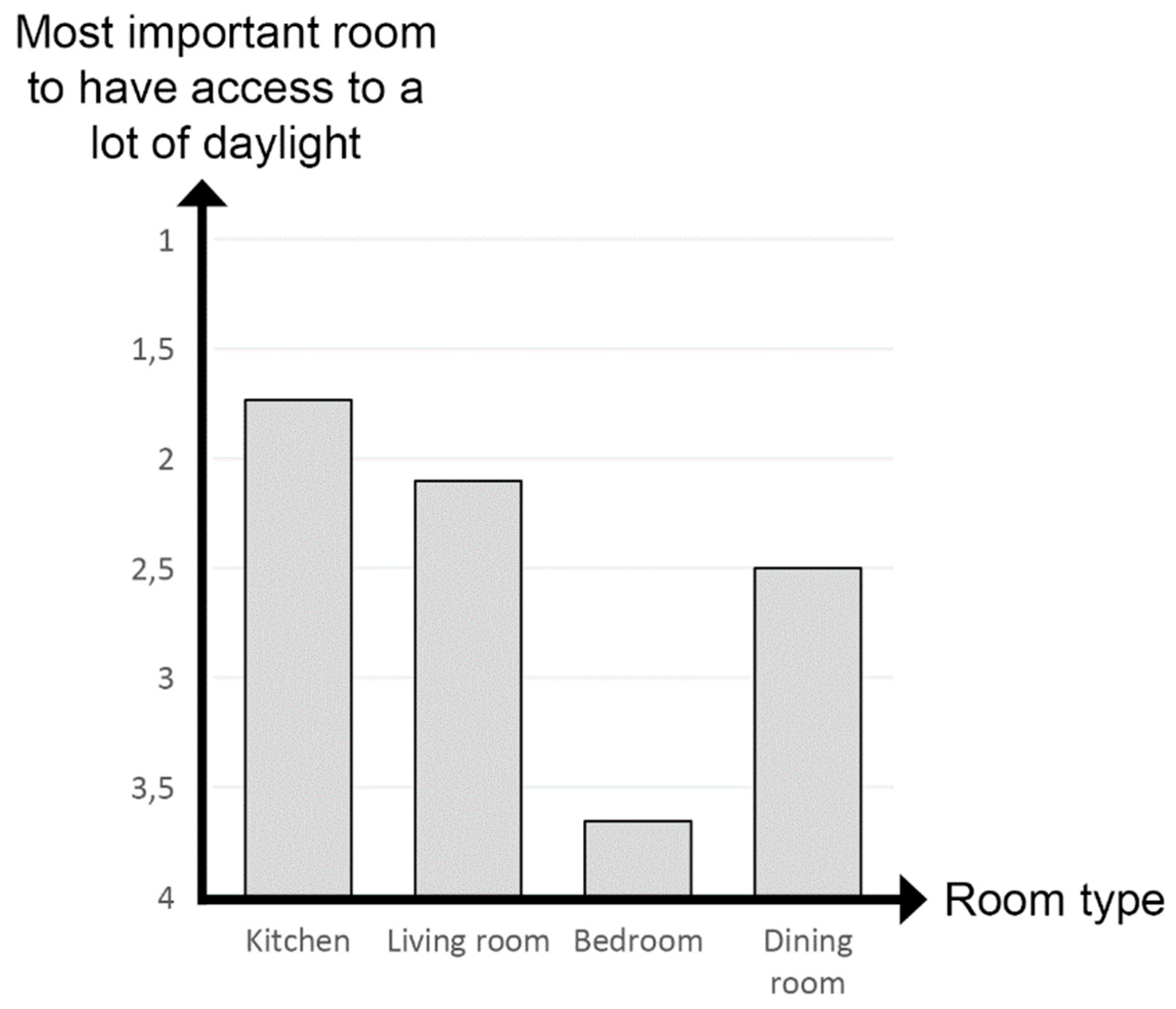
- Q3.
- Which room type do you think is the most important room to have the greatest access to daylight?
- Q4.
- Do you normally use electrical lighting daytime in the following rooms?
- Q5.
- Do you have access to direct sunlight in the following rooms?
- Q6.
- Do you often use curtains, blinds or other sun shadings in the following rooms?
- Q7.
- In case of using a sun shading, why is it used?
- Q8.
- Do you consider the view out to be interesting in the following rooms? (Quantity)
- Q9.
- Do you consider the view out to be enough in the following rooms? (Quality)
3. Results: Simulated DFP in the Sample Buildings
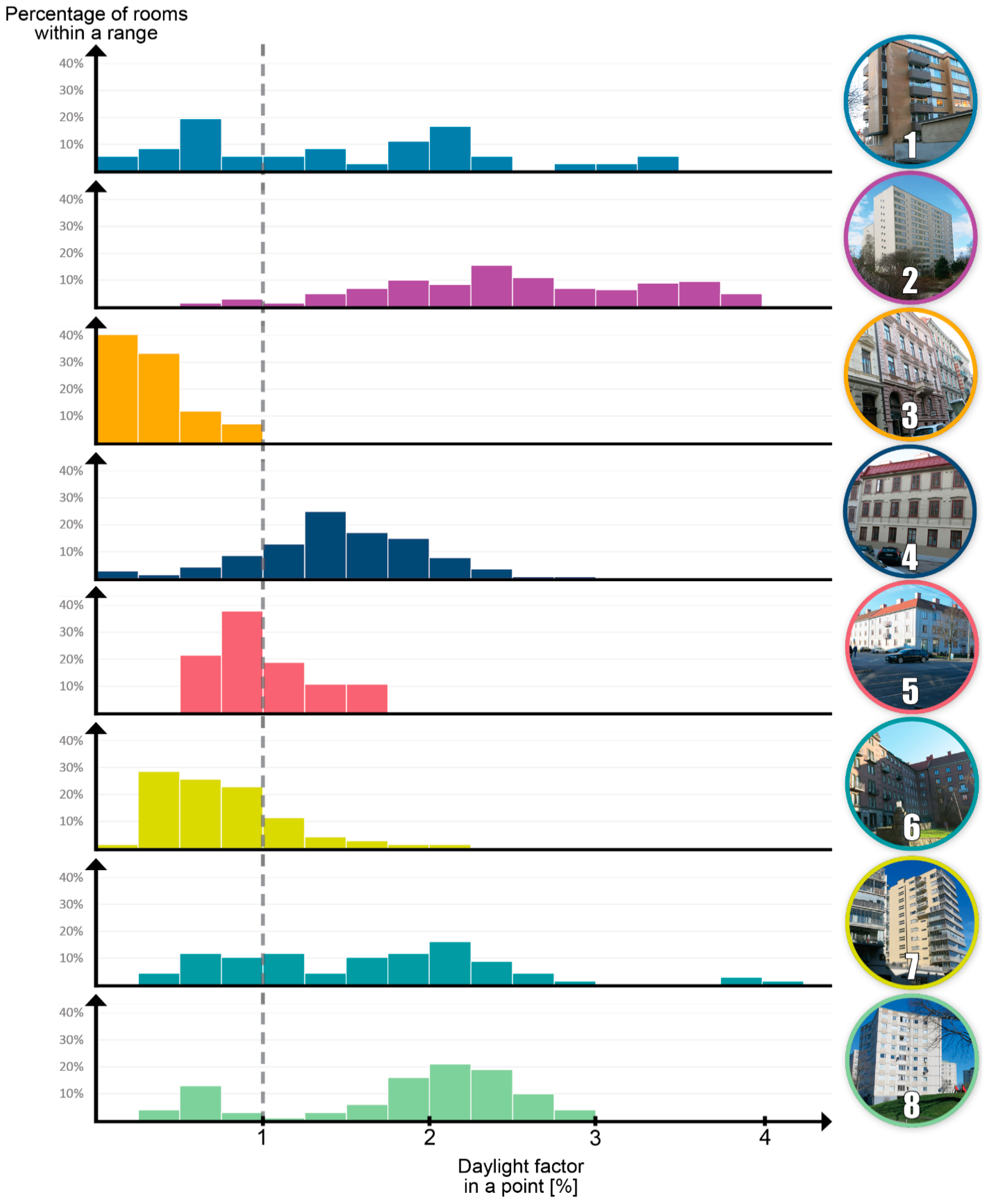
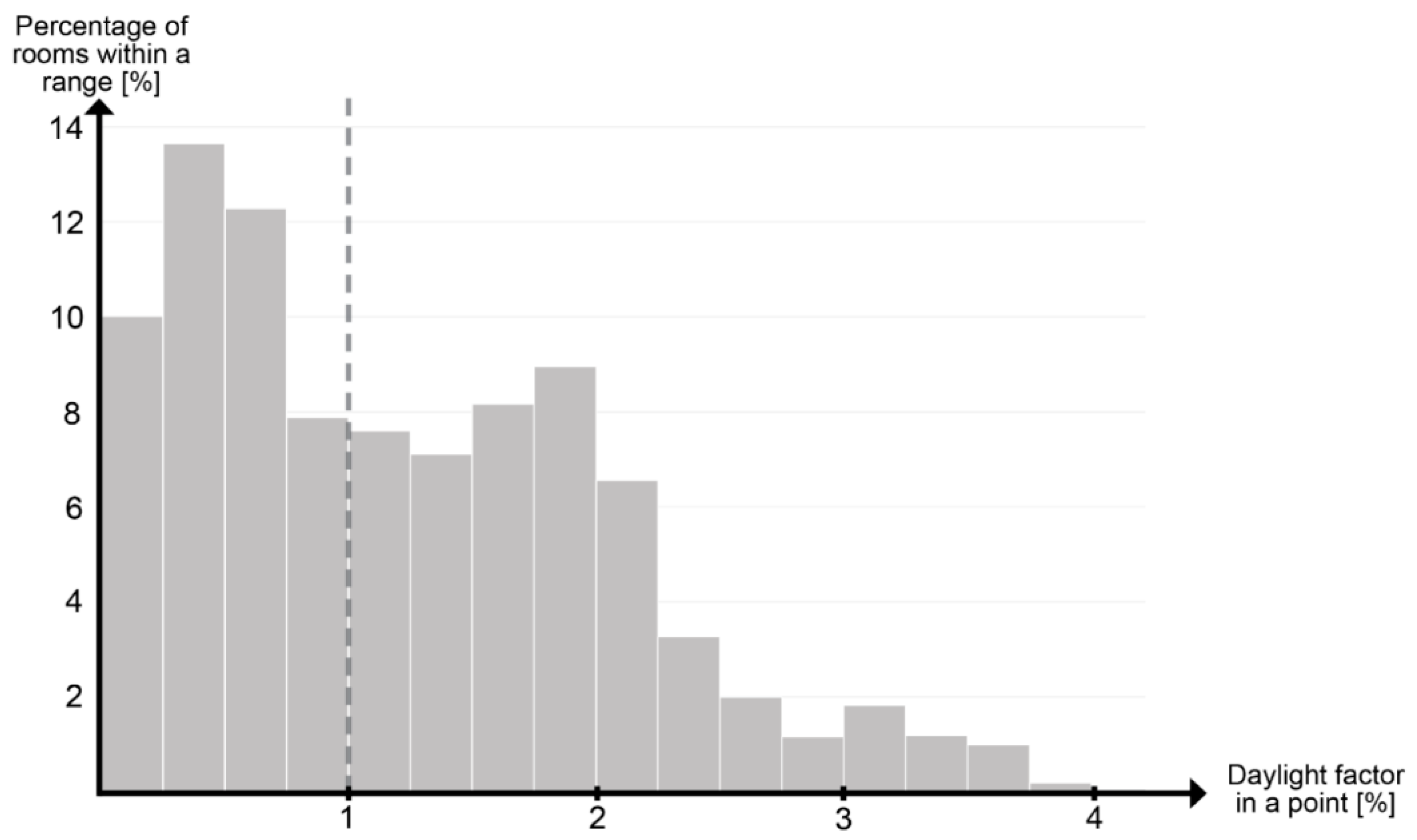
3.1. Residential Buildings (IDs 1–8)
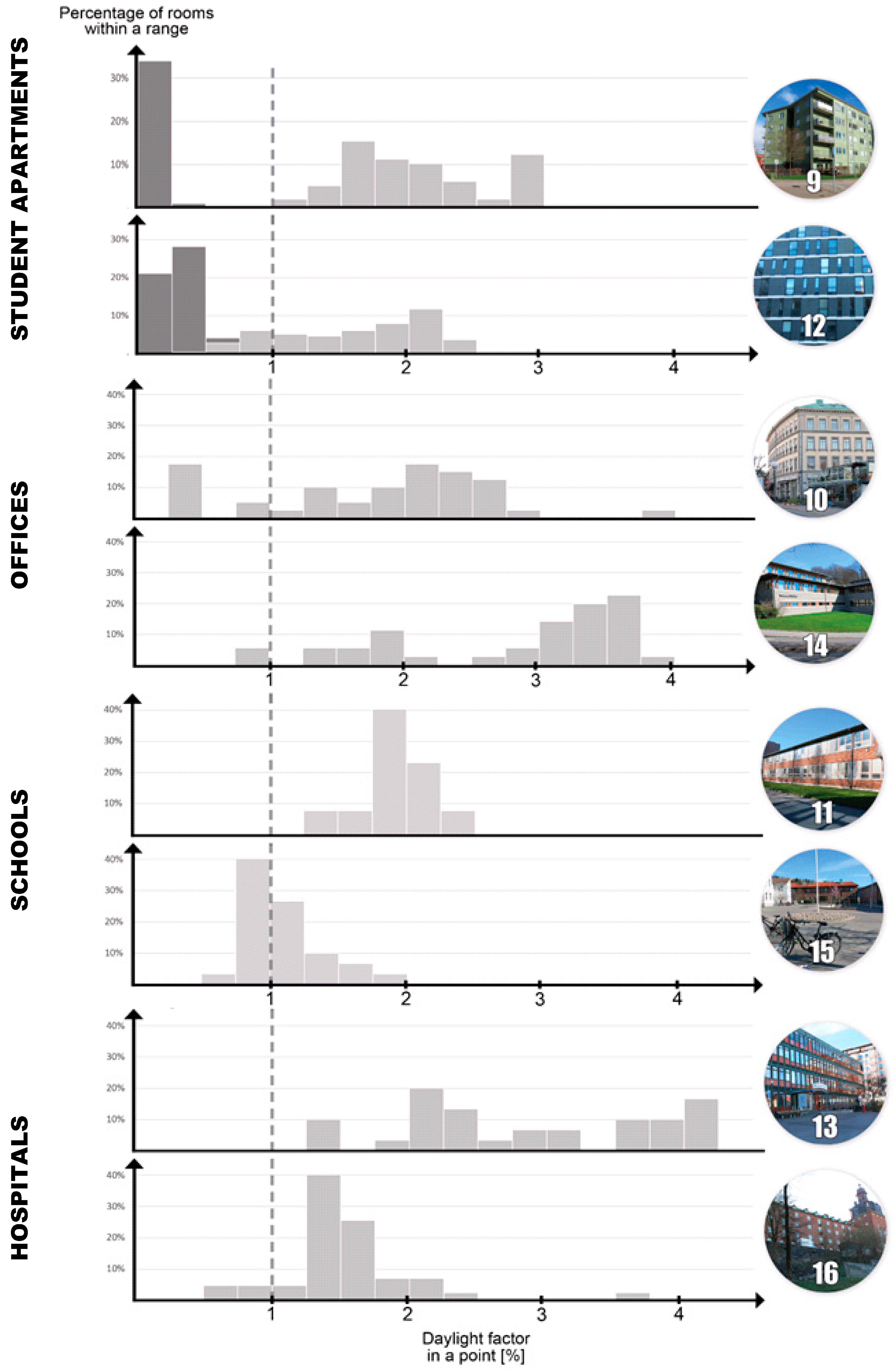
3.2. Non-Residential Buildings (ID 9 to ID 16)
4. Results – Correlation Between Different DF Metrics
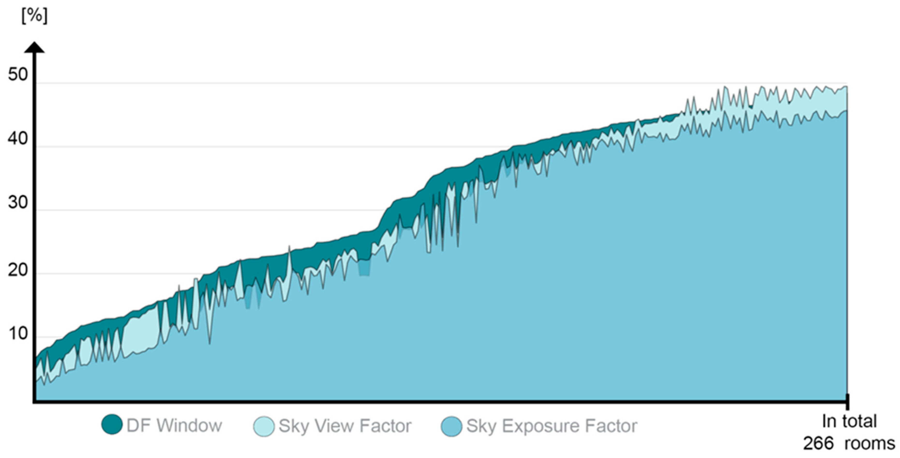
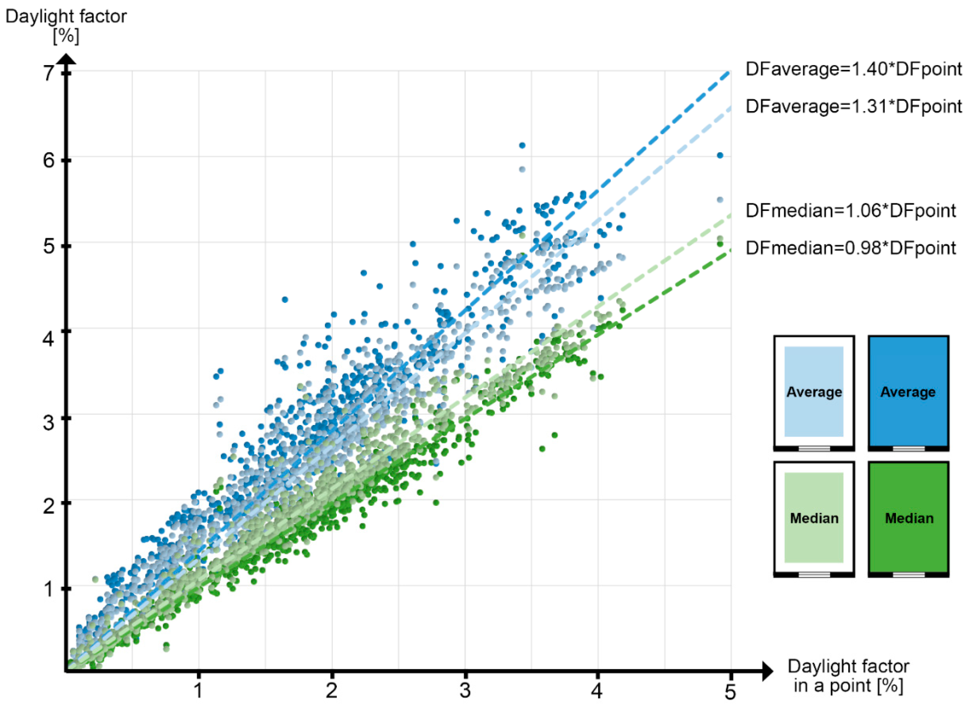
4.1. Correlation Between , and
4.2. Correlation Between and AF
4.3. Correlation Between Daylight Factors Indoors and
4.4. Correlation Between DFP and Results of the Field Survey
5. Conclusions
Author Contributions
Funding
Acknowledgments
Conflicts of Interest
References
- Boverket. SBN 1975 Svensk Byggnorm. 1975. Available online: https://www.boverket.se/contentassets/c4c3f9ae57294ae889bfaf710b08b125/sbn-1975-utg-3.pdf (accessed on 30 May 2019).
- Xue, P.; Mak, C.M.; Cheung, H.D. The effects of daylighting and human behavior on luminous comfort in residential buildings: A questionnaire survey. Build. Environ. 2014, 81, 51–59. [Google Scholar] [CrossRef]
- Cheung, H.D.; Chung, T.M. A study on subjective preference to daylit residential indoor environment using conjoint analysis. Build. Environ. 2008, 43, 2101–2111. [Google Scholar] [CrossRef]
- Cantin, F.; Dubois, M.-C. Daylighting metrics based on illuminance, distribution, glare and directivity. Light. Res. Technol. 2011, 43, 291–307. [Google Scholar] [CrossRef]
- Boverket. BBR Boverket’s building regulations. BFS 2011:6 with amendments up to 2018:4 (in Swedish). 2018. Available online: https://www.boverket.se/globalassets/publikationer/dokument/2018/bbr-2018_konsoliderad-version.pdf (accessed on 30 May 2019).
- Rogers, P.; Tillberg, M.; Bialecka-Colin, E.; Österbring, M.; Mars, P. En Genomgång av Svenska Dagsljuskrav 2015. Available online: http://www.acc-glas.se/wp-content/uploads/2013/12/SBUF-12996-Slutrapport-Förstudie-Dagsljusstandard.pdf (accessed on 30 May 2019).
- Boverket. Housing, Internal Migration and Economic Growth in Sweden. (In Swedish). 2016. Available online: https://www.boverket.se/globalassets/publikationer/dokument/2016/housing-internal-migration-and-economic-growth-in-sweden.pdf (accessed on 30 May 2019).
- Strømann-Andersen, J.; Sattrup, P. The urban canyon and building energy use: Urban density versus daylight and passive solar gains. Energy Build. 2011, 43, 2011–2020. [Google Scholar] [CrossRef]
- Robinson, A.; Selkowitz, S. Tips for Daylighting with Windows. Available online: https://buildings.lbl.gov/sites/default/files/ellen_thomas_lbnl-6902e.pdf (accessed on 14 April 2019).
- Eriksson, S.; Waldenström, L. Daylight in Existing Buildings A Comparative Study of Calculated Indicators for Daylight. Master’s Thesis, Chalmers University of Technology, Gothenburg, Sweden, 2016. [Google Scholar]
- Rogers, P.; Dubois, M.-C.; Tillberg, M.; Östbring, M. Moderniserad Dagsljusstandard. no. SBUF ID: 13209. 2018. Available online: http://www.acc-glas.se/wp-content/uploads/2013/12/SBUF-12996-Slutrapport-Förstudie-Dagsljusstandard.pdf (accessed on 30 May 2019).
- Mardaljevic, J.; Christoffersen, J. A Roadmap for Upgrading National/EU Standards for Daylight. In Proceedings of the CIE Centenary Conference “Towards a New Century of Light“, Paris, France, 15–16 April 2013; pp. 1–10. [Google Scholar]
- Reinhart, C.; Breton, P.-F. Experimental validation of 3DS MAX ® DESIGN 2009 and DAYSIM 3.0 1 2. In Proceedings of the 11th International IBPSA Conference, Glasgow, Scotland, 27–30 July 2009. [Google Scholar]
- Mardaljevic, J.; Andersen, M.; Roy, N.; Christoffersen, J. Daylighting metrics for residential buildings. In Proceedings of the 27th Session CIE, Sun City, South Africa, 11–15 July 2011; p. 18. [Google Scholar]
- Hellinga, H.; Hordijk, T. The D&V analysis method: A method for the analysis of daylight access and view quality. Build. Environ. 2014, 79, 101–114. [Google Scholar]
- Yu, X.; Su, Y. Daylight availability assessment and its potential energy saving estimation -A literature review. Renew. Sustain. Energy Rev. 2015, 52, 494–503. [Google Scholar] [CrossRef]
- Tregenza, P. Uncertainty in daylight calculations. Light. Res. Technol. 2017, 49, 829–844. [Google Scholar] [CrossRef]
- SIS. SS 914201 Building design - Daylighting - Simplified method for checking required window glass area; SIS Swedish Standards Institute: Stockholm, Sweden, 1988. [Google Scholar]
- Velux. Daylight Visualizer. 2019. Available online: https://www.velux.com/article/2016/daylight-visualizer (accessed on 30 May 2019).
- Radsite. Radiance. 2019. Available online: https://www.radiance-online.org// (accessed on 20 April 2016).
- SGBC. Miljöbyggnad 3.0; Sweden Green Building Council: Stockholm, Sweden, 2017. [Google Scholar]
- Ecolabelling, N. Small Houses, Apartment Buildings and Buildings for Schools and Pre-Schools. 2016. Available online: https://www.ecolabel.dk/kriteriedokumenter/089e_2_11.pdf (accessed on 20 March 2016).
- Mata, É.; Kalagasidis, A.S.; Johnsson, F. Energy usage and technical potential for energy saving measures in the Swedish residential building stock. Energy Policy 2013, 55, 404–414. [Google Scholar] [CrossRef]
- Yu, X.; Su, Y.; Chen, X. Application of RELUX simulation to investigate energy saving potential from daylighting in a new educational building in UK. Energy Build. 2014, 74, 191–202. [Google Scholar] [CrossRef]
- Mardaljevic, J. Simulation of annual daylighting profiles for internal illuminance. Light. Res. Technol. 2000, 32, 111–118. [Google Scholar] [CrossRef]
- Li, D.; Cheung, G. Average daylight factor for the 15 CIE standard skies. Light. Res. Technol. 2006, 38, 137–152. [Google Scholar] [CrossRef]
- Li, D.H.W.; Wong, S.L. Daylighting and energy implications due to shading effects from nearby buildings. Appl. Energy 2007, 84, 1199–1209. [Google Scholar] [CrossRef]
- Dubois, M.-C.; Flodberg, K. Daylight utilisation in perimeter office rooms at high latitudes: Investigation by computer simulation. Light. Res. Technol. 2013, 45, 52–75. [Google Scholar] [CrossRef]
- Thomsen, K.E.; Rose, J.; Mørck, O.; Jensen, S.Ø.; Østergaard, I.; Knudsen, H.N.; Bergsøe, N.C. Energy consumption and indoor climate in a residential building before and after comprehensive energy retrofitting. Energy Build. 2016, 123, 8–16. [Google Scholar] [CrossRef]
- Li, D.; Wong, S.; Tsang, C.; Cheung, G.H. A study of the daylighting performance and energy use in heavily obstructed residential buildings via computer simulation techniques. Energy Build. 2006, 38, 1343–1348. [Google Scholar] [CrossRef]
- Bournas, I.; Dubois, M.-C. Daylight regulation compliance of existing multi-family apartment blocks in Sweden. Build. Environ. 2019, 150, 254–265. [Google Scholar] [CrossRef]
- Jacobsson, E.; Eriksson, F. Evaluation of Sun-and Daylight Availability in Early Stages of Building Development A Method Based on Correlations of Interior and Exterior Metrics. Master’s Thesis, Chalmers University of Technology, Gothenburg, Sweden, 2017. [Google Scholar]
- Reinhart, C.F.; Lagios, K.; Niemasz, J.; Jakubiec, A. DIVA for Rhino Version 2.0. 2011. Available online: http://www.diva-for-rhino.com/ (accessed on 30 April 2016).
- Chalmers Geodata Portal. Available online: https://geodata.chalmers.se/ (accessed on 22 April 2019).
- Bellia, L.; Pedace, A.; Fragliasso, F. The impact of the software’s choice on dynamic daylight simulations’ results: A comparison between Daysim and 3ds Max Design®. Sol. Energy 2015, 122, 249–263. [Google Scholar] [CrossRef]
- Jones, N.L. Validated Interactive Daylighting Analysis for Architectural Design. Ph.D. Thesis, Massachusetts Institute of Technology, Cambridge, MA, USA, 2017. [Google Scholar]
- Nocera, F.; Faro, A.L.; Costanzo, V.; Raciti, C. Daylight Performance of Classrooms in a Mediterranean School Heritage Building. Sustainability 2018, 10, 3705. [Google Scholar] [CrossRef]
- SIS. “SS-EN 17037-2018 Daylight in buildings.”; SIS Swedish Standards Institute: Stockholm, Sweden, 2018. [Google Scholar]


| ID | Characteristics | Year | Use | Total Number of Floors | Number of Evaluated Floors | Number of Evaluated Rooms |
|---|---|---|---|---|---|---|
| 1 | Elongated apartment block | 1972 | R | 6 | 4 | 36 |
| 2 | Tower block | 1960 | R | 12 | 8 | 200 |
| 3 | Townhouse with a courtyard | 1887 | R | 4 | 4 | 42 |
| 4 | Governor’s house with a courtyard | 1897 | R | 4 | 3 | 140 |
| 5 | Governor’s house with a courtyard | 1923 | R | 3 | 3 | 37 |
| 6 | L-shaped apartment block | 1928 | R | 6 | 5 | 70 |
| 7 | Compact tower block | 2013 | R | 11 | 4 | 68 |
| 8 | Compact tower block | 1960 | R | 10 | 4 | 100 |
| 9 | Compact block | 2004 | SA | 5 | 3 | 97 |
| 10 | Townhouse with two street sides | 1863 | O | 5 | 4 | 47 |
| 11 | Low-rise, elongated | 1962 | S | 2 | 2 | 14 |
| 12 | L-shaped compact block | 2006 | SA | 13 | 5 | 230 |
| 13 | Low-rise compact block | 1966 | H | 4 | 4 | 38 |
| 14 | Low-rise, indented top floor | 2006 | O | 3 | 3 | 36 |
| 15 | U-shaped, low-rise with a school yard | 2001 | S | 2 | 2 | 30 |
| 16 | Block with a tower on one side | 1927 | H | 4 | 3 | 52 |
| Total | 1237 |
| Object | Reflectance | Object | Reflectance |
|---|---|---|---|
| Outside ground | 0.2 | Window frame | 0.8 |
| External façades | 0.3 | Side of window | 0.5 |
| Surrounding buildings and objects | 0.2 | Balcony | 0.3 |
| Floor | 0.3 | Balcony bottom | 0.7 |
| Walls | 0.7 | Water | 0.5 |
| Ceiling | 0.8 | Roof | 0.3 |
| ID | Number of Distributed Surveys | Number of Collected Surveys | Response Rate |
|---|---|---|---|
| 2 | 36 | 24 | 67% |
| 6 | 15 | 8 | 53% |
| 7 | 16 | 13 | 81% |
| All | 67 | 45 | 67% |
| Building ID | Percentage of All Rooms with a DF > 1% | Average DF for a Building |
|---|---|---|
| 1 | 61% | 1.47% |
| 2 | 96% | 2.50% |
| 3 | 0% | 0.31% |
| 4 | 83% | 1.45% |
| 5 | 41% | 1.01% |
| 6 | 21% | 0.74% |
| 7 | 74% | 1.65% |
| 8 | 80% | 1.85% |
| Average for all rooms/buildings | 71% | 1.67% |
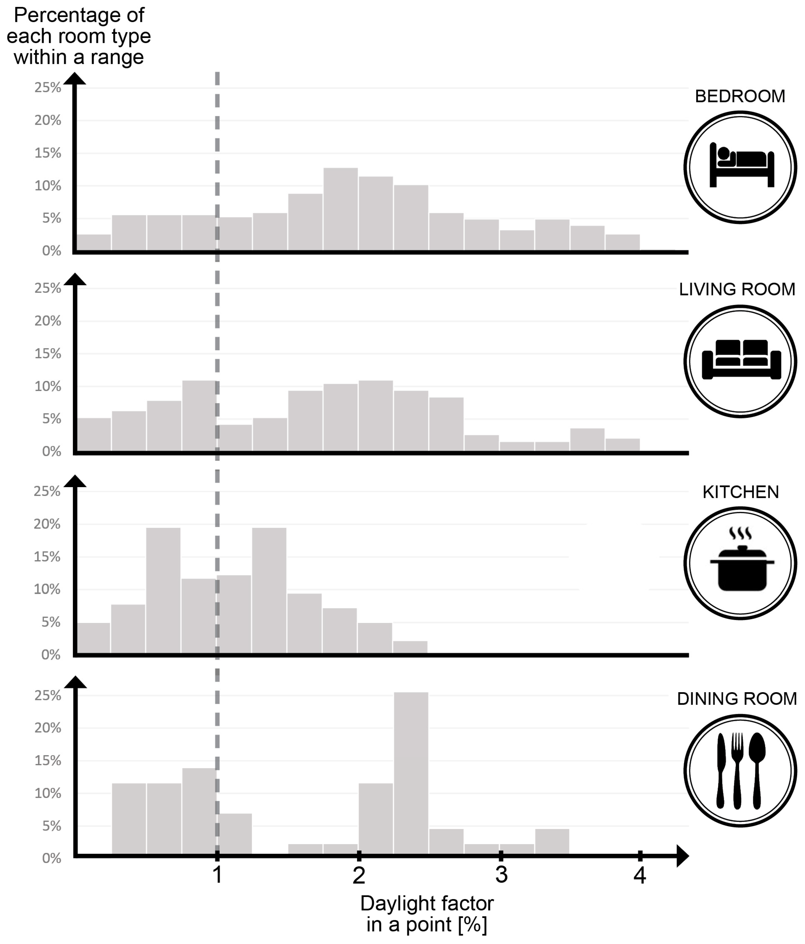
| Bedroom | Living Room | Kitchen | Dining Room |
|---|---|---|---|
| Bedroom | Living room | Kitchen | Dining room |
| Small room | Family room | Divided kitchen | Divided dining |
| Living room/Bedroom | Divided kitchenette | ||
| Living room/Kitchen | Living room/Kitchen |
| Results for AF | Results for | Percentage of the Studied Rooms | Agreement between the Methods |
|---|---|---|---|
| ≥ 1% | 70% | Yes | |
| < 1% | 8% | Yes | |
| < 1% | 12% | No | |
| ≥ 1% | 10% | No |
© 2019 by the authors. Licensee MDPI, Basel, Switzerland. This article is an open access article distributed under the terms and conditions of the Creative Commons Attribution (CC BY) license (http://creativecommons.org/licenses/by/4.0/).
Share and Cite
Eriksson, S.; Waldenström, L.; Tillberg, M.; Österbring, M.; Sasic Kalagasidis, A. Numerical Simulations and Empirical Data for the Evaluation of Daylight Factors in Existing Buildings in Sweden. Energies 2019, 12, 2200. https://doi.org/10.3390/en12112200
Eriksson S, Waldenström L, Tillberg M, Österbring M, Sasic Kalagasidis A. Numerical Simulations and Empirical Data for the Evaluation of Daylight Factors in Existing Buildings in Sweden. Energies. 2019; 12(11):2200. https://doi.org/10.3390/en12112200
Chicago/Turabian StyleEriksson, Sara, Lovisa Waldenström, Max Tillberg, Magnus Österbring, and Angela Sasic Kalagasidis. 2019. "Numerical Simulations and Empirical Data for the Evaluation of Daylight Factors in Existing Buildings in Sweden" Energies 12, no. 11: 2200. https://doi.org/10.3390/en12112200
APA StyleEriksson, S., Waldenström, L., Tillberg, M., Österbring, M., & Sasic Kalagasidis, A. (2019). Numerical Simulations and Empirical Data for the Evaluation of Daylight Factors in Existing Buildings in Sweden. Energies, 12(11), 2200. https://doi.org/10.3390/en12112200