Modeling, Simulationand Analysis of On-Board Hybrid Energy Storage Systems for Railway Applications ^†

Abstract

In this paper, a decoupled model of a train including an on-board hybrid accumulation system is presented to be used in DC traction networks. The train and the accumulation system behavior are modeled separately, and the results are then combined in order to study the effect of the whole system on the traction electrical network. The model is designed specifically to be used with power flow solvers for planning purposes. The validation has been carried out comparing the results with other methods previously developed and also with experimental measurements. A detailed description of the power flow solver is beyond the scope of this work, but it must be remarked that the model must by used with a solver able to cope with the non-linear and non-smooth characteristics of the model. In this specific case, a modified current injection-based power flow solver has been used. The solver is able to incorporate also non-reversible substations, which are the most common devices used currently for feeding DC systems. The effect of the on-board accumulation systems on the network efficiency will be analyzed using different real scenarios.

1. Introduction

The use of power flow algorithms for planning traction networks is a widely-accepted technique [1,2]. However, the use of accurate models of the network and the trains may result in very complicated simulations [3]. In [4], the authors proposed a methodology to perform a fast estimation of the aggregated railway power system and traffic performance. In [5], for instance, the authors tried to reduce the computational burden of the whole simulation, proposing a compression technique that reduces the number of necessary simulations for evaluating the performance of the traction network. In [6], the energetic macroscopic representation (EMR) was used in order to simplify the development of the train and network mathematical models. This approach has been use extensively. For instance, in [7], the authors compared different traction substation models. The models presented using the EMR were extremely accurate and precise [8], and they may describe every single part of the system and are appropriate for applications in which the transient behavior of the trains is critical, such as hardware in the loop applications [9]. A very detailed model of an electric train fed by supercapacitors connected to fuel cells was presented in [10]. Pseudo-static models have been traditionally less accurate, but much faster [11]. They are usually combined with power flow solvers that must be able to manage the complex non-smooth and non-derivable characteristics presented by the new power electronic devices installed within the railways [12].

In this paper, a very simple model for representing a train equipped with a hybrid energy storage system is presented. The combination of regenerative braking with the energy storage system is presented as one of the most effective ways to increase the overall efficiency of traction systems [13,14,15]. Schedule optimization together with these sets of technologies can be the key to very important energy savings [16,17,18]. In [19], the savings derived from the installation of an energy storage device in a diesel-electric locomotive were also evaluated. In [20], a method for optimization of the size of the storage devices in order to maximize the energy recovered by the regenerative braking system was presented. An accurate sizing of all the elements in the system was critical for a proper energy management within the system [21,22,23]. In other cases, the storage systems were installed off-board at the substation level [24]. Many applications, like the one presented in this paper, use hybrid energy storage systems based on batteries and ultracapacitors; usually, the battery covers a base load, and the ultracapacitors are used for feeding the peak power. In order to connect two different storage technologies to the same train, specific power electronic topologies are being investigated, the most common being the DC/DC converter that connects the DC traction network with the storage devices, which uses IGBT technology with a topology that allows the interleaved multi-channel buck-boost operation principle. This converter can adapt the voltage in the energy storage to the catenary voltage. This configuration provides the flexibility required by the operating conditions. Sometimes, series connection of the ultracapacitors or battery packs is needed in order to achieve a specific voltage level. Usually, there are parallel connected IGBT branches that can be fired at the same time or we can shift the firing to reduce the current ripple. In the case of hybrid energy storage systems, there are IGBT branches connected to the battery packs and other IGBT branches connected to the ultracapacitors. Other hybrid topologies use also a common connection; in these cases, the battery packs share the common bus of the ultracapacitors. Usually, buck mode is used for charging the ultracapacitors and the battery. In this situation, the converter drivers control the upper IGBTs, keeping open the devices placed at the bottom of the branch. The current flows from the train DC bus to the energy storage modules. The boost mode (for discharging) uses the IGBTs placed in the bottom, keeping open the ones at the top of the branch. This will produce a current flow from the energy storage devices to the train DC bus. The results obtained using the pseudostatic simulations proposed in this paper are a valuable input for the designers of the energy storage devices. However, a detailed description of the power electronic topology or the storage technology is far beyond the scope of this paper. In order to determine the size of the battery and the ultracapacitors, it is necessary to assess the performance of the system using an ideal integrated energy storage system like the one presented in this paper.

Wayside energy storage can be an alternative to the on-board accumulation systems and in some cases can also be better. In [12,25], the authors mentioned that for choosing the correct infrastructure/train configuration, multiple cases should be analyzed, and all possible technologies should be compared, like for instance reversible substations, wayside energy storage, and on-board energy storage. In order to take advantage of the power regenerated by the trains, the most common solution used in the past was: (1) to optimize the schedule, so when one train is accelerating, another train is braking (this solution is quite difficult to achieve without automatic driving systems); (2) the use of reversible substations; in this case, railway manufacturers are quite reluctant to change the conventional non-controlled diode-based substations because they are inexpensive and robust, so nearly all reversible substations are formed with an IGBT bridge in parallel with the diode bridge; the infrastructure keeps using the diodes to transfer power from AC to DC, and they use the IGBT to put power back into the DC system. Currently, with the drastic reduction in the prices of energy storage systems, it is not clear which is going to be the solution that will prevail, reversibility or accumulation. Probably, accumulation will be a much more reasonable solution in the near future since it helps to maintain the voltages in the DC traction network within the limits, but also increases the overall efficiency of the system. In [25], different configurations were compared, and we can observe that on-board and wayside energy storage are better solutions in terms of efficiency. On-board accumulation is slightly better in terms of efficiency because the losses in the DC system are slightly lower, but wayside energy storage can be more cost-effective since a single accumulation device can be shared by all the trains in the system. Similar conclusions were obtained in [26]; in this work, the use of wayside energy storage improved the overall efficiency by more than 20% and also improved the controllability and the voltage profile of the network. Similar conclusions were obtained in [24,27] supporting the previous conclusions. In [24], the use of energy storage at the substation level reduced the annual cost of energy by 13%. We would like to point out that the main contribution of this paper is the mathematical model; a detailed comparison between the infrastructure alternatives considering wayside and on-board energy storage and reversible substations is beyond the scope of the work, which is focused specifically on providing an accurate and efficient model to simulate on-board energy’storage.

What this work presents is a decoupled model that considers the train and the storage system as separate devices located at the same electrical point and interacting with each other and with the network. The authors did not consider the input filter, and the losses in this device can be estimated and added to the electromechanical and electrochemical device. This approach reduces the complexity of the mathematical model without reducing the accuracy when compared with previous proposed models [28]. The model has been embedded in a commercial software package that uses a modified current injection method to solve the power flow problem [12]; the solver allows combining regenerative trains with diode-based non-reversible substations. It must be remarked that even when there is the possibility of combining regenerative trains with Voltage Source Converter (VSC)-based reversible substations [29,30], in the vast majority of the cases, the existing infrastructures and also the new ones use non-controlled and non-reversible substations due to their robustness, reliability, and low cost [31]. The combination of the two technologies must be done carefully. It should be noticed that without a very precise coordination, the power regenerated by one train could be used to feed another train, but if there is no power demand when the train is regenerating, the voltage in the network will increase, and the substations will be blocked. In such cases, usually the voltage limit is reached, and most of the regenerated power must be burned in the rheostatic braking system. The use of on-board accumulation systems could alleviate this situation [32]. However, it will be demonstrated, the size and effectiveness of the storage system depend highly on the trains’ power profile and the schedule.

The results obtained using this kind of simulations are very useful also to study how the accumulation systems are cycled in real applications. There are many on-going research projects that try to predict the life of the accumulation systems depending on the cycling. For instance, the common thought is that load leveling the charge and discharge of the battery packs can contribute to extending the life of the batteries. Recent studies revealed unexpected results. In [33], the authors cycled LiNiCoAl and LiFePO₄ modules with 18,650 cells 750 times in a period of six months, and they concluded that the degradation was higher with constant current loads than using dynamic pulse profiles. There is still much research to do in this direction, and every new storage technology requires these kinds of studies. The output of the pseudo-static simulation could be a valuable input for the researchers that try to reproduce real dynamic cycles in accumulation systems.

In the next section, the mathematical model of the train plus the energy storage device in different working modes is explained. Section 3 presents the results obtained using the proposed model in a real traction network. This section has four subsections: in the first three subsections, we describe the feeding infrastructure, the rolling stock, and the proposed scenarios. In the last subsection a deep analysis of the results is presented. Conclusions are stated in Section 4.

2. Mathematical Model of the Train and the Storage System

The proposed train model including the storage system has been simplified in order to lighten the computational burden. In [28], the storage system and the traction equipment of the train were considered as a single element; in this case, the storage system and the traction system separation will substantially simplify the solving procedure. This simplification in the model will not reduce the accuracy because both models are equivalent. The time savings in simulation were around 20%. The solving procedure in this case allows the decoupling between the storage system and the traction equipment, and this is the main reason for this simplification in the mathematical model. From now on, we will use the term train when referring to the traction and breaking device, and storage will be reserved for the accumulation device. Both devices will be modeled as separate, but coupled models.

The storage control will consider the train behavior, as well as the catenary voltage, so we will assume that the train and the storage will be traveling along the grid separated, but connected to the same catenary point.

The joint power and current can be easily calculated as the sum of the current of the train and the storage. For the sign criteria, we will consider that the train will have positive current and power in traction mode when it is absorbing power from the electric grid. In the other case, the storage will have positive power and current when it is in discharging mode. In Figure 1a,b, the schematic representation of the train and storage mathematical models is depicted in traction and braking modes, respectively. We only consider two situations that are the most common ones, the train in traction mode with the storage system discharging and the train in braking mode with the storage system in charging mode.

2.1. Train Plus Storage Working in Traction Mode

The behavior of the train and the storage in traction mode is summarized in Figure 1a, and the functions $f_{t1}$, $g_{d1}$, and $g_{d2}$ are depicted in the curves presented in Figure 2a–c. In the next subsections, a detailed description of the train and the storage model will be presented.

2.1.1. Train Behavior (Positive Power in Traction Mode)

The train model will read first the power reference provided by the external software; we will refer to this power as the mechanical reference power ($P_{mech,ref}^{train}$). It is possible to use coupled models that generate the mechanical power reference during the electrical simulation [34]. However, in most of the cases, the train mechanical model and the electrical problem are solved separately. To obtain the train electrical reference power ($P_{ref}^{train}$), the mechanical power will be divided by the efficiency of the electromechanical conversion that will include the motors, converters, and the rest of the equipment. This efficiency will be labeled as train efficiency in traction mode (${\nu }_t^{train}$). This operation can be executed before launching the solver with all positive powers provided by the external software package, so the input file for the solver will already consider this efficiency according to the next expression:

$$P_{ref}^{train}=\frac{P_{mech,ref}^{train}}{{\nu }_t^{train}}$$

(1)

It must be pointed out that this electric power reference ($P_{ref}^{train}$) is not the final electric power that the train will demand from the grid ($P^{train}$). The overcurrent protection can limit the power requested from the grid when the catenary voltage ($V_{cat}$) is very low for protection purposes.

Each train will have two configuration parameters to set the overcurrent protection ($V_{reg,t}^{train}$ and $V_{min}^{train}$); in Figure 2a, the function $f_{t1}$ is depicted, and the mathematical expression of such function is expressed in (2).

As can be observed, the actual power consumed by the train depends on the catenary voltage and the train electric power reference, as well as the parameters that define the overcurrent protection ($P^{train}=f_{t1}(P_{ref}^{train},V_{reg,t}^{train},V_{min}^{train},V_{cat})$).

$$P^{train}=\left\{\begin{array}{cc}0\hfill & V_{cat}\le V_{min}^{train}\hfill \\ \frac{V_{cat}-V_{min}^{train}}{V_{reg,t}^{train}-V_{min}^{train}}{P}_{ref}^{train}\hfill & V_{min}^{train}<V_{cat}<V_{reg,t}^{train}\hfill \\ P_{ref}^{train}\hfill & V_{cat}\ge V_{reg,t}^{train}\hfill \end{array}\right.$$

(2)

2.1.2. Storage Behavior (Negative Power in Traction Mode)

The maximum amount of power that can be extracted from the primary active power source of the storage system (ultracapacitors, batteries, flywheel, or whatever other technology used) is labeled as $P_{max}^{STO}$ and depends on the level of charge of the storage system ($E^{STO}$) with the function $g_{d1}$ (see Figure 2b) that is expressed in (3).

$$P_{max}^{STO}=\left\{\begin{array}{cc}{P}_{rated,d}^{STO}\hfill & E^{STO}\le E_{reg,d}^{STO}\hfill \\ \frac{E^{STO}}{E_{reg,d}^{STO}}{P}_{rated,d}^{STO}\hfill & E^{STO}>E_{reg,d}^{STO}\hfill \end{array}\right.$$

(3)

The maximum discharging power will be zero if the energy stored is zero, and it will increase in a linear way until a specific energy level is achieved ($E_{reg,d}^{STO}$). The maximum discharging power will be constant for the interval between $E_{reg,d}^{STO}$ and the maximum energy that the system can store ($E_{max}^{STO}$). This maximum power ($P_{max}^{STO}$) can be calculated at each instant once the storage energy level is updated, but before launching the power flow algorithm, because it is independent of the catenary voltage and the train behavior.

The maximum power available from the storage primary source ($P_{max}^{STO}$) has to be multiplied by the electrochemical conversion process efficiency in discharging mode (${\nu }_d^{STO}$) to obtain the maximum available electric power to be injected into the system ($P_{max,av}^{STO}$). This operation can be also executed before launching the power flow solver.

$$P_{max,av}^{STO}={\nu }_d^{STO}{P}_{max}^{STO}$$

(4)

Due to the storage system overcurrent protection, the maximum available power could be constrained if the voltage is too low by means of the function $g_{d2}$ (see Figure 2c). The output of this function is the actual available power that the storage device can inject into the system considering already the catenary voltage constraint ($P_{av}^{STO}$). To define the function $g_{d2}$, we need to define also the regulation parameters ($V_{reg}^{STO}$ and $V_{min}^{STO}$). The analytical expression of the function can be found in (5). Each train can have different regulation parameters. In the case of the storage system, these two parameters will be common for charging and discharging mode.

$$P^{train}=\left\{\begin{array}{cc}0\hfill & V_{cat}\le V_{min}^{STO}\hfill \\ \frac{V_{cat}-V_{min}^{STO}}{V_{reg}^{STO}-V_{min}^{STO}}{P}_{max,av}^{STO}\hfill & V_{min}^{STO}<V_{cat}<V_{reg}^{STO}\hfill \\ P_{max,av}^{STO}\hfill & V_{cat}\ge V_{reg}^{STO}\hfill \end{array}\right.$$

(5)

2.1.3. Coupling between the Train, Storage, and Network

Regarding the interaction between the train, the storage device, and the grid, many operational philosophies can be considered. In this particular case, one of the most popular working modes in real applications has been adopted, giving priority to the energy extraction from the storage system. When the train demands a given amount of power, if this power is available in the accumulation system, it is going to be extracted from it. If not, the train will extract the available power from the storage system, and the rest will be imported from the network. With this control philosophy, the actual power that the storage system is going to inject into the system is going to be calculated following the next expression:

$$P^{STO}=min(P^{train},P_{av}^{STO})$$

(6)

Due to the employed power flow solving procedure [11], we will use the previous iteration of the catenary voltage to calculate first the power of the train ($P^{train}$), then we will calculate the storage power ($P^{STO}$). The catenary net power, representing the whole set (train plus storage device), can be calculated as $P^{cat}=P^{train}-P^{STO}$. Once the catenary power is calculated, a new iteration of the power flow will be launched to obtain a new value of the catenary voltage. The simulation will stop once the difference between all catenary voltages in all nodes in two successive iterations is lower than a specific tolerance.

Once the convergence is achieved, the energy level at the storage system must be updated using the following expression:

$$E_{t+1}^{STO}=E_t^{STO}-(1/{\nu }_d^{ACR})·\mathsf{\Delta }t·P^{ACR}$$

(7)

2.2. Train Plus Storage Working in Braking Mode

An analogous procedure can be used for describing the train and the storage device working in braking mode. Such behavior is summarized in Figure 1b and the functions $f_{b1}$, $g_{c1}$, and $g_{c2}$ depicted in the curves represented in Figure 2d–f. In the next subsections, a detailed description of the train and the storage model will be presented.

2.2.1. Train Behavior (Positive Power in Traction Mode)

Again, the train model will read first the power reference provided by the external software ($P_{mech,ref}^{train}$). To obtain the train electrical reference power ($P_{ref}^{train}$), the mechanical power will be multiplied by the efficiency of the electromechanical conversion (see Equation (8)). This efficiency will be labeled as the train efficiency in braking mode (${\nu }_b^{train}$).

$$P_{ref}^{train}={\nu }_b^{train}{P}_{mech,ref}^{train}$$

(8)

The squeeze control can limit the power requested from the grid when the catenary voltage ($V_{cat}$) is very high for protection purposes. Each train will have two configuration parameters to set the squeeze control ($V_{reg,b}^{train}$ and $V_{max}^{train}$). In Figure 2d, the function $f_{b1}$ is depicted. The mathematical expression of such a function is expressed in (9). As can be observed, the actual power that the train is going to regenerate depends on the catenary voltage and the train electric power reference, as well as the parameters that define the overcurrent protection ($P^{train}=f_{b1}(P_{ref}^{train},V_{reg,b}^{train},V_{max}^{train},V_{cat})$).

$$P^{train}=\left\{\begin{array}{cc}{P}_{ref}^{train}\hfill & V_{cat}\le V_{reg,b}^{train}\hfill \\ \frac{V_{cat}-V_{max}^{train}}{V_{reg,t}^{train}-V_{max}^{train}}{P}_{ref}^{train}\hfill & V_{reg,b}^{train}<V_{cat}<V_{max}^{train}\hfill \\ 0\hfill & V_{cat}\ge V_{max}^{train}\hfill \end{array}\right.$$

(9)

2.2.2. Storage Behavior (Negative Power in Braking Mode)

The maximum amount of power that can be injected into the primary active power source of the storage system ($P_{max}^{STO}$) depends on the level of charge of the storage system ($E^{STO}$) with the function $g_{c1}$ (see Figure 2e) that is expressed in (10).

$$P_{max}^{STO}=\left\{\begin{array}{cc}\frac{E^{STO}-E_{max}^{STO}}{E_{reg,c}^{STO}-E_{max}^{STO}}{P}_{rated,c}^{STO}\hfill & E^{STO}\le E_{reg,d}^{STO}\hfill \\ P_{rated,d}^{STO}\hfill & E^{STO}>E_{reg,d}^{STO}\hfill \end{array}\right.$$

(10)

Again, this maximum power ($P_{max}^{STO}$) can be calculated at each instant once the storage energy level is updated, but before launching the power flow algorithm, because it is independent of the catenary voltage and the train behavior.

The maximum power that could be injected into the storage referring to the catenary side of the storage system ($P_{max,av}^{STO}$) has to be calculated using the electrochemical conversion process efficiency in charging mode (${\nu }_c^{STO}$) according to (11). This operation can be also executed before launching the power flow solver.

$$P_{max,av}^{STO}=\frac{P_{max}^{STO}}{{\nu }_d^{STO}}$$

(11)

The overcurrent protection of the storage system is considered also in braking mode using the function $g_{c2}$ (see Figure 2f). The output of this function is the actual available power that the storage device can extract from the system considering already the catenary voltage constraint ($P_{av}^{STO}$). To define the function $g_{c2}$, we need to define also the regulation parameters ($V_{reg}^{STO}$ and $V_{min}^{STO}$). The analytical expression of the function is similar to the one for the traction mode (see Equation (5)).

2.2.3. Coupling between the Train, Storage, and Network

To be consistent with the control philosophy previously described, the system will assign priority to the energy injection into the storage system. When the train regenerates a given amount of power, the storage system will try to use it (if possible) to increase its energy level. If not, the train will inject the maximum allowed power into the storage system, and the rest will be injected into the network. The actual power that the storage system is going to use for charging is going to be calculated following the next expression:

$$P^{STO}=max(P^{train},P_{av}^{STO})$$

(12)

The catenary net power, representing the whole set (train plus storage device) can be calculated as $P^{cat}=P^{train}-P^{STO}$. At each instant, the energy level of the storage system can be calculated as follows:

$$E_{t+1}^{STO}=E_t^{STO}-{\nu }_c^{STO}·\mathsf{\Delta }t·P^{STO}$$

(13)

3. Results’ Analysis

In this section, we will analyze in depth the effect of the on-board accumulation system on the trains and network behavior in different scenarios. This section will have four subsections. In the first one, we will describe the basic feeding infrastructure, lines, and substations. In the second subsection, we will describe the rolling stock used in the simulations. The third subsection will be focused on the description of the different scenarios that will be analyzed in Section 4.

3.1. Feeding Infrastructure

The case study in this article will focus on the study of a real network consisting of two lines of 30.84 km and 36.93 km. The voltage level of the system was 3000 V. The simplified diagram of the network can be observed in Figure 3. Line blue is the longest; it had nine stops and four electrical nodes labeled as S1, S2, S3, and S4. The red line shared the first two electrical nodes with the blue line, and it had 17 stops and six electrical nodes labeled as S1, S2, S3, S4, S5, and S6. There were a total of eight electrical nodes and seven lines. Among the eight nodes, only three of them represented feeding substations; the rest were just nodes without any connection with the AC system. The three substations were placed in the nodes S3 and S5 of the red line and in the node S3 of the blue line. The three substations had the same characteristics. All of them were composed by a power transformer with rated power of 3 MW and a short circuit voltage of 5%; the no load output voltage of the rectifier was 3000 V, and the voltage at rated load (1000 A) was 2880 V. The equivalent impedance of each of the three substations in forward mode (AC to DC) was 270 m$\mathsf{\Omega }$. The equivalent impedance of the overhead conductor and the rails (return circuit) were respectively 28.605 m$\mathsf{\Omega }$/km and 7 m$\mathsf{\Omega }$/km. In

Table 1. Length of the different line segments in km.

	S1 to S2	S2 to S3	S3 to S4	S4 to S5	S5 to S6
Red Line	4.316	0.500	13.800	7.848	4.378
Blue Line	4.316	25.284	7.335	-	-

, the lengths of the different segments of the red and blue lines can be observed.

3.2. Rolling Stock

The train used in both lines was an electrical multiple unit (EMU). The whole unit was 2.940 m wide 4.265 m high and had a total length of 98.05 m, with an unladen weight of 157.3 t. The units were composed of five cars, the two ends having a driver’s cabin and a normal floor. The middle car had a normal floor, while the other two cars had a low floor. The five cars were supported on two types of bogies, the trailer bogie and the tractor. The tractor bogie was always shared between two cars. The train was designed to use a standard Iberian track gauge (1668 mm) at a maximum speed of 120 km/h with almost 1000 passengers, although it could reach 160 km/h with minor modifications. The maximum total power of the train was 2.2 MW, and it had regenerative braking. In the base case, the trains were not going to be equipped with on-board energy storage systems. However, we considered the possibility of adding an on-board accumulator system based on a hybrid battery/ultracapacitor technology. The power profiles obtained during the simulation in the accumulation system would help the manufacturer to determine the percentage of energy that must be stored in the battery or ultracap parts. The electromechanical efficiency of the trains in traction and braking modes (${\nu }_t^{train},{\nu }_b^{train}$), as well as the electrochemical efficiency of the storage system in charging and discharging modes (${\nu }_c^{STO},{\nu }_d^{STO}$) were set to $0.95$. The total accumulation system capacity ($E_{max}^{STO}$) was 7 kWh, and the on-board energy storage device rated charging and discharging power ($P_{rated,c}^{STO},P_{rated,d}^{STO}$) was 1 MW.

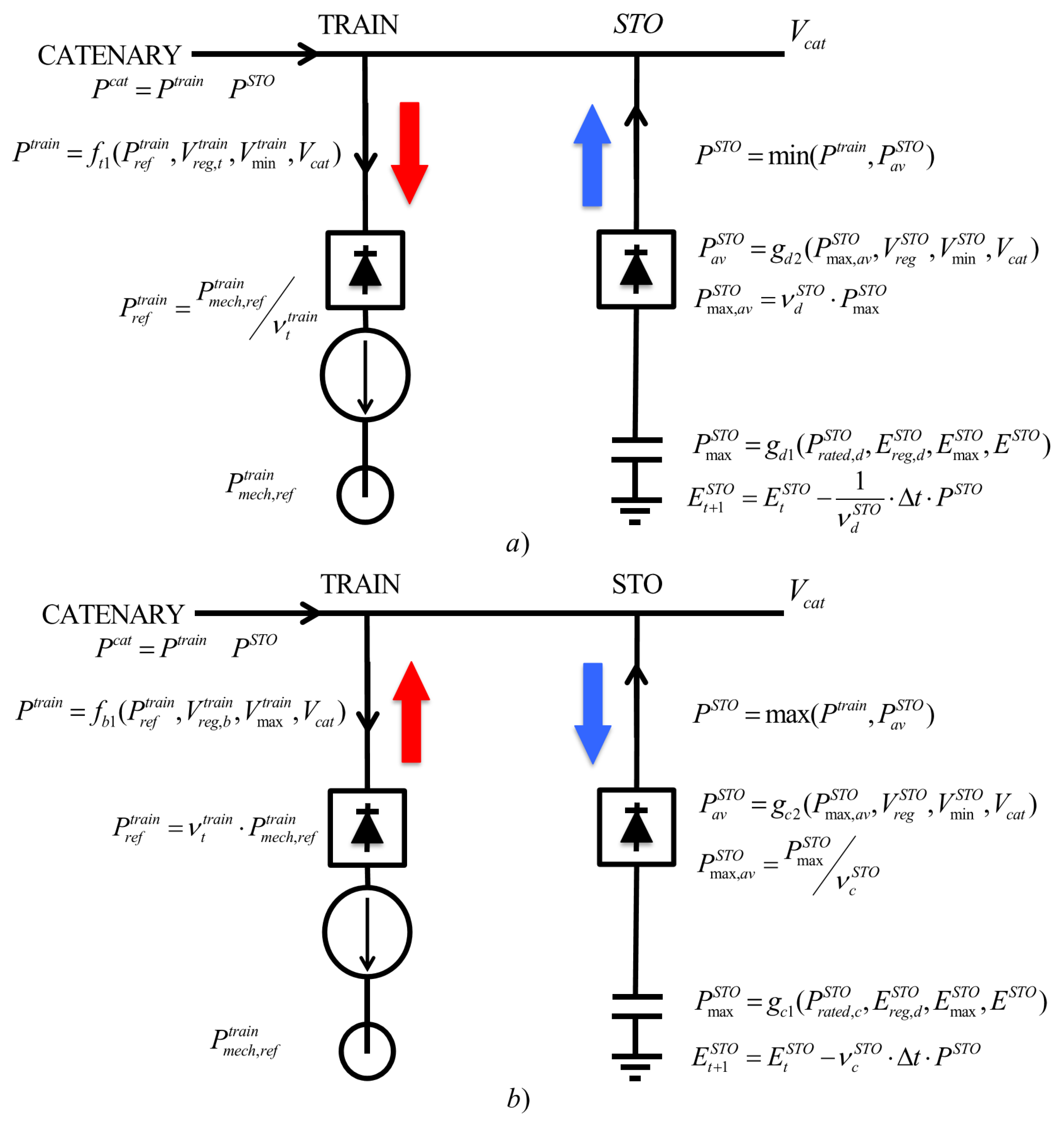
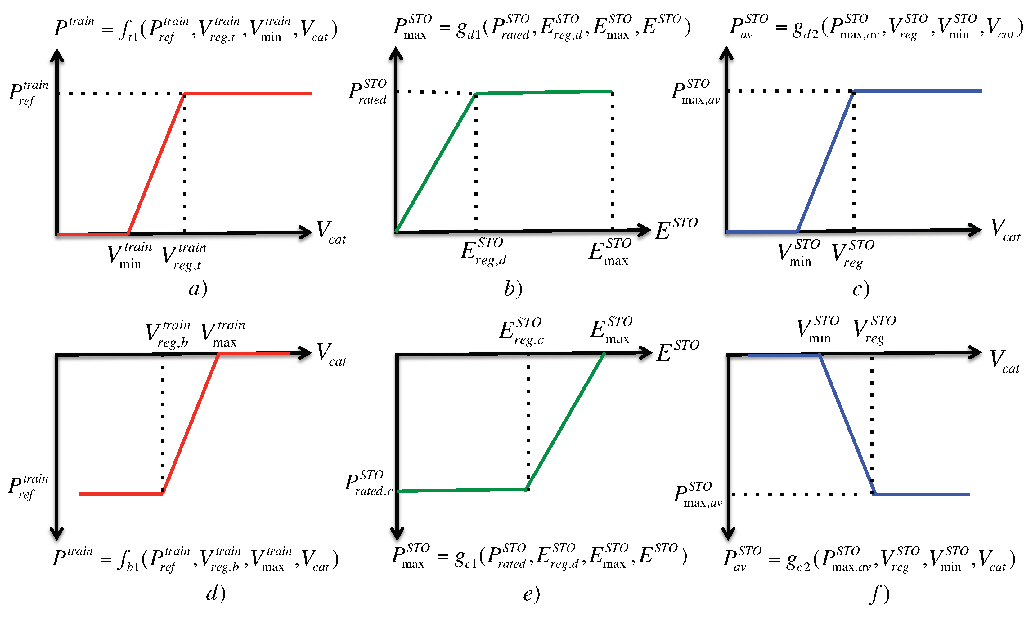
Regarding the protection curves of the trains and the storage elements, the minimum and the regulation voltage of the train in traction mode ($V_{min}^{train},V_{reg,t}^{train}$) were set to 1980 V and 2280 V. The same values have been selected for the minimum and regulation voltage of the energy storage system ($V_{min}^{STO},V_{reg}^{STO}$). In braking mode, the regulation voltage and the maximum voltage of the squeeze control ($V_{max}^{train},V_{reg,b}^{train}$) were 3300 V and 3600 V, respectively. In the cases in which the on-board accumulation system was activated, the system would be initialized with no charge.

In

Table 2. Summary of the train behavior in the different trips; all data are in kWh.

Trip	Required Mechanical Energy	Mechanical Regeneration Capacity	Required Electrical Energy	Electrical Regen. Capacity	Min. Electrical Consump. Theoretical
S1 to S6 Red	245	112	258	106	151
S6 to S1 Red	240	107	253	102	151
S1 to S4 Blue	243	61	256	58	198
S4 to S1 Blue	187	99	197	94	103
Average Trip	229	95	241	90	151

, the data summarizing the behavior of the trains in the different trips are collected. In the first column, we can observe the required mechanical power to complete the trip. It can be seen that the slope of the blue line was steeper because the difference between the power required for outward and return journeys was greater than on the red line. The average trip considering the two lines and both directions needed 229 kWh. The mechanical regeneration capacity in Column 2 is the available mechanical power that can be regenerated. Columns 3 and 4 contain the required electrical power and the electrical regeneration capacity considering already the efficiency of the electromechanical conversion. The electrical regeneration capacity was usually around 40% of the required electrical power, except in the S1 to S4 trip of the blue line. In this case, because the train ascended a steep slope, the regeneration capacity was much lower, around 22% of the required electrical power. In the fifth column, we can see the minimum electric consumption. This consumption was calculated as the required electrical power minus the electrical regeneration capacity. Off course, this is a theoretical consumption that considers that we took advantage of all electrical power available for regeneration. This is not true, mainly because of two reasons. First, part of the power that was available to be injected into the catenary was burned in the rheostatic braking system when the squeeze control was activated in order to maintain the catenary voltage below the maximum level. In addition, if the train was equipped with on-board accumulation, the efficiency of the electrochemical conversion during the charging and discharging process also reduced the percentage of available regenerated power that could be reused. For these reasons, we uses these minimum consumption figures as a theoretical ceiling to compare the different solutions, but we must be aware of the fact that we will not reach this theoretical ceiling.

3.3. Description of the Selected Scenarios

The authors developed eight different scenarios to study the influence of the accumulation system on the network, as can be observed in

Table 3. Summary of the different proposed scenarios.

Scenario Code	Traffic Density	On-Board Acc.System	Trains Headset (min)	Trains per Route	Number of Trains	Sim.Time (h:mm)
L0	Light	No	50	10	40	8:18
L1	Light	Yes	50	10	40	8:18
M0	Medium	No	35	14	56	8:23
M1	Medium	Yes	35	14	56	8:23
D0	Dense	No	20	24	96	8:28
D1	Dense	Yes	20	24	96	8:28
H0	Heavy	No	10	47	188	8:28
H1	Heavy	Yes	10	47	188	8:28

. There were four different paths for the trains, from S1 to S6 and from S6 to S1 for the red line and from S1 to S4 and from S4 to S1 for the blue line. Four different traffic densities were considered. Light traffic scenarios used a train headset of 50 min with 10 departures for each of the above-described routes. The medium traffic scenario considered a train headset of 35 min with 14 departures per route. The dense traffic scenario launched 24 trains per route with a headset of 20 min. Finally, the heavy traffic scenario launched 47 trains per route with a headset of 10 min. The simulation interval was very similar for all scenarios, and it went from eight hours and 18 min for the light traffic scenario to eight hours and 28 min for the heavy traffic scenario. Each of the four traffic densities were simulated without and with on-board accumulation systems without modifying the feeding infrastructure. The obtained results are presented in the next section and will clarify the effect of the on-board accumulation systems on the railway traction networks depending on the density of the traffic.

3.4. Analysis of the Results

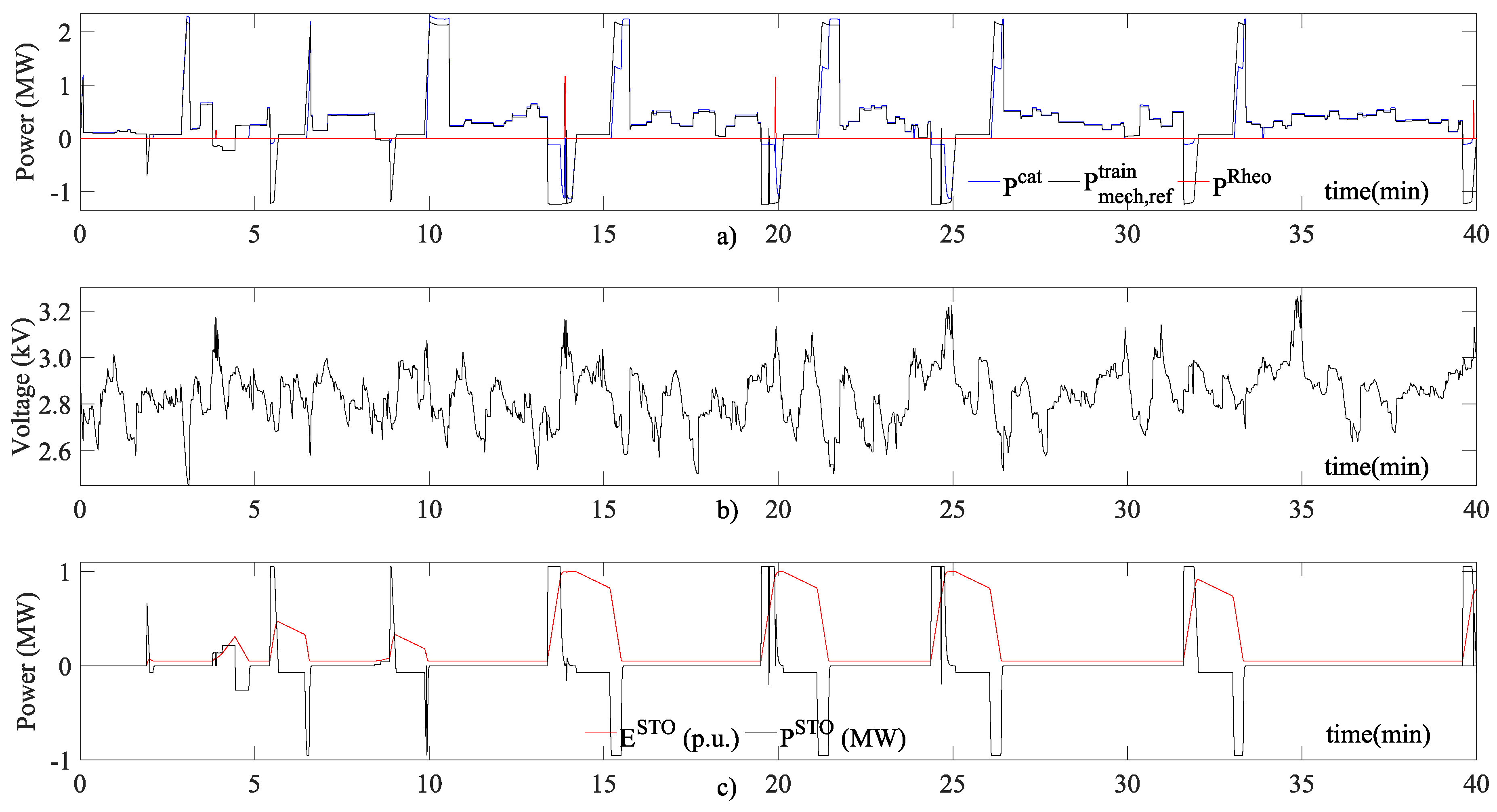
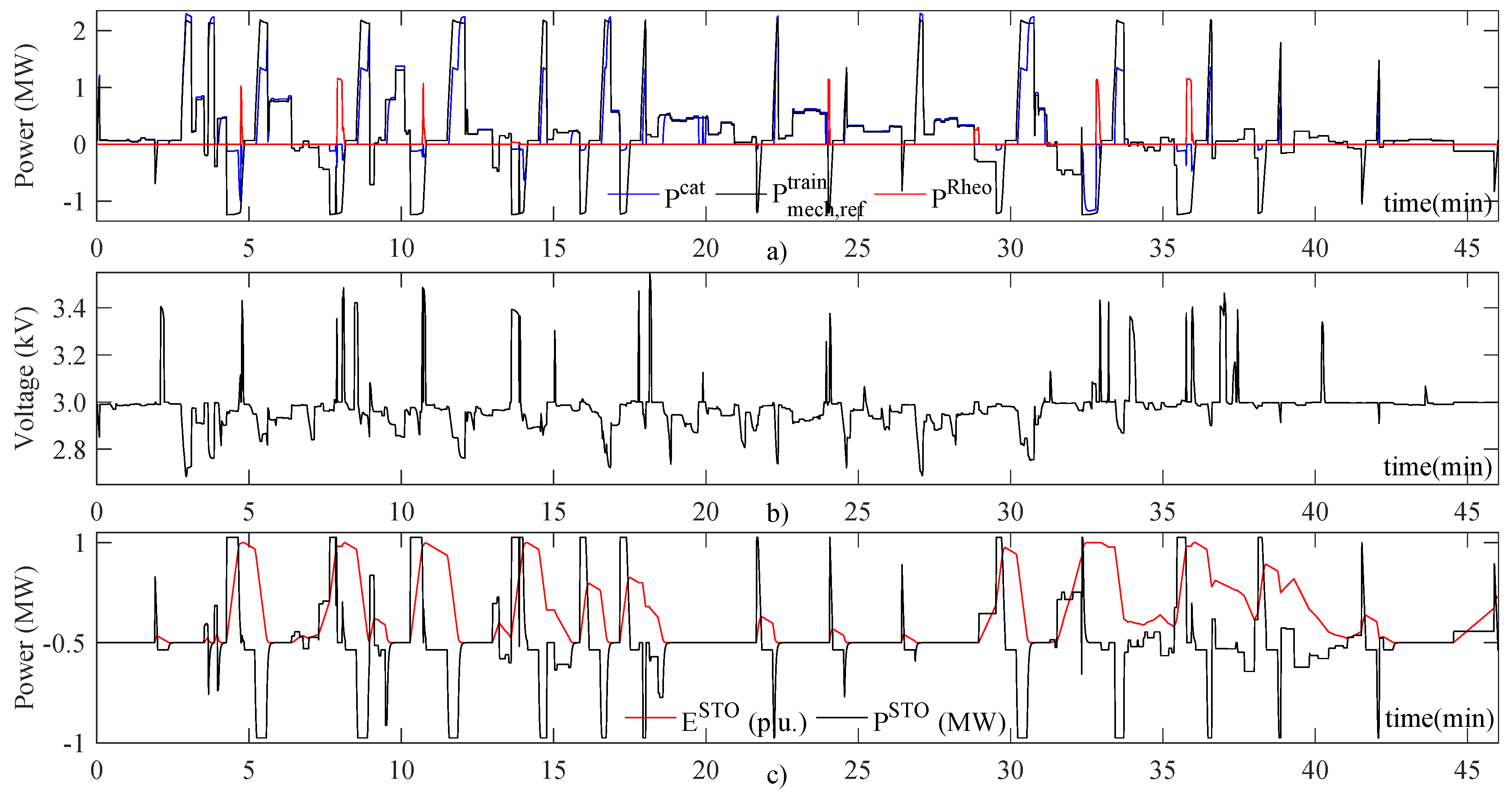
The above-described scenarios were simulated, and the obtained results are analyzed in this subsection. With the software used for simulation, we can obtain time-varying series of each electrical variable in the train or in the feeding network. An example of this detailed analysis can be observed in Figure 4, in which Train Number 4 on the red line route starting from S1 is represented in Scenario L1. It must be noticed how on seven occasions, the train burned part of the regenerated energy using the rheostatic system due to the high catenary voltage, even when the train was equipped with an energy storage system and the storage capacity was not full. It can be observed also how the power extracted/injected into the catenary differed from the train mechanical reference due to the efficiency of the electromechanical conversion process, but also because part of the power was provided by the energy storage system. In Figure 5, the fourth train of the blue line starting from S1 is represented, in this case for the heavy traffic scenario (H1). It has to be remarked that the voltage level was much lower and the network receptivity higher. The burned power in this scenario was nearly zero since the overvoltage protection was only activated on four occasions with a very short duration.

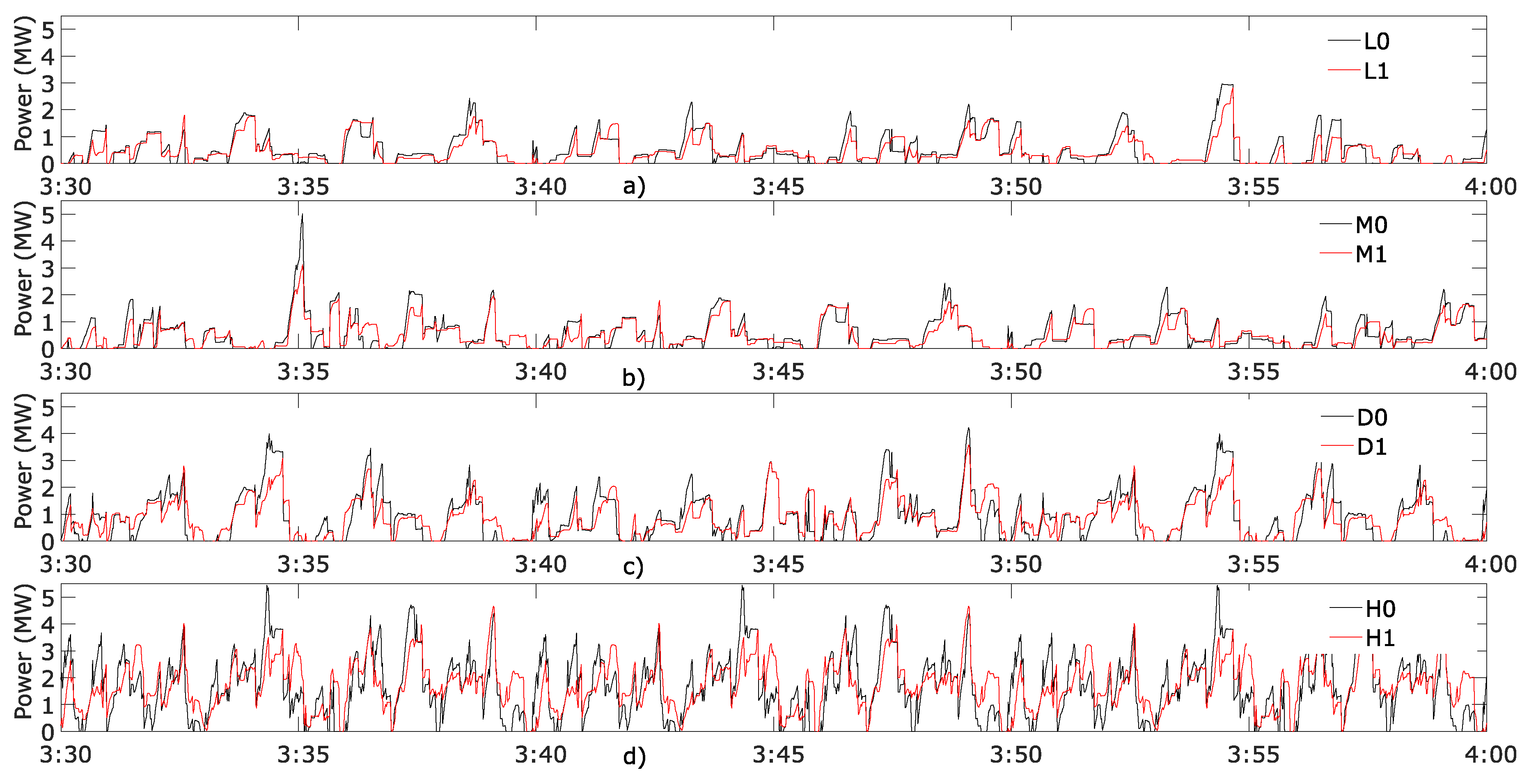
The analysis of the time-varying curves was very interesting since it showed how electrical variables were correlated and it helped to understand the mathematical model proposed in the previous sections. However, in order to determine the effectiveness of the combination of the trains plus the infrastructure, another kind of analysis must be carried out. In Figure 6 is represented the power extracted from the AC network at substation S5 of the red line during the first four hours of simulation for all scenarios. Each subfigure represents two scenarios with the same train headset, but with and without the accumulation system. The correlation between the power extracted from the AC network was higher in the low traffic scenarios. 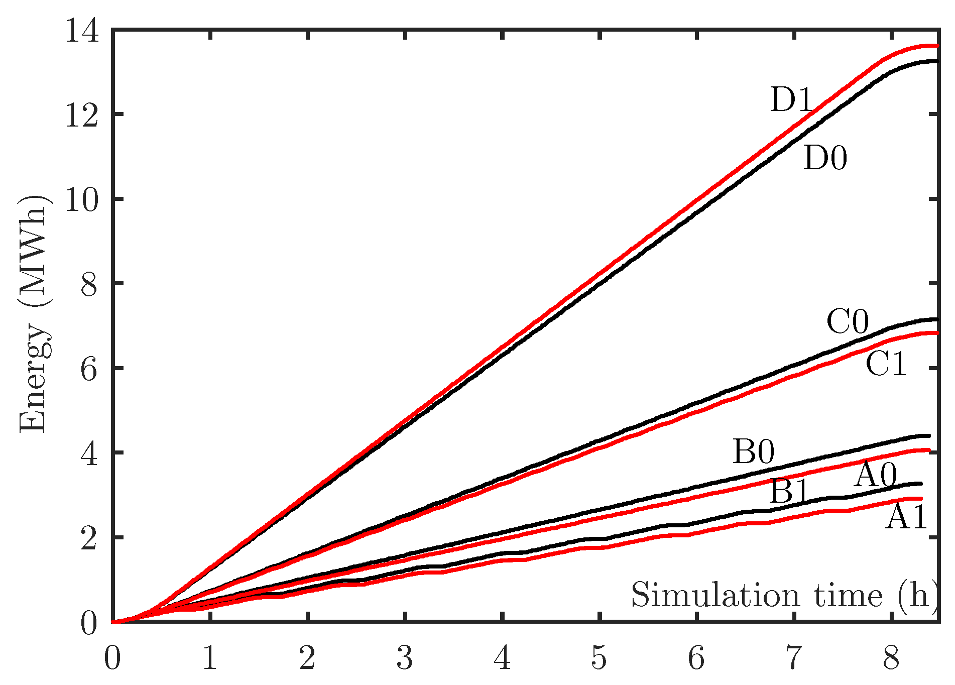Figure 7 depicts the energy extracted from the AC network at substation S5 in the eight possible scenarios. It must be noticed that the red solid line represents always the scenarios with energy storage. Obviously, scenarios with the same traffic were quite correlated. It should be pointed out that in the light, medium, and dense traffic scenarios, the energy consumption from the AC network in the cases with energy storage systems was a little bit lower. Paradoxically, that is not the case for the heavy traffic scenario in which the energy consumed from the AC network was higher when the trains were equipped with energy storage systems. As will be observed, in heavy traffic scenarios, it was more efficient to share the energy surplus with other trains than storing it in the on-board accumulation system.

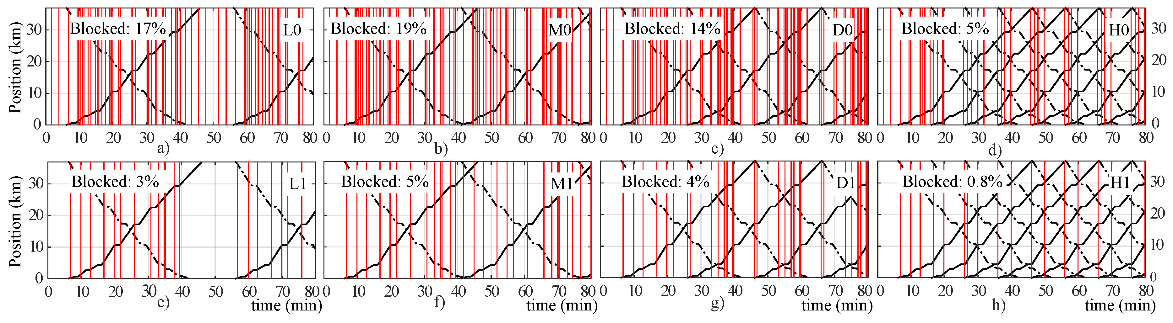
In Figure 8, we represent the Marey diagrams of each scenario just for the red line. The horizontal axis represents time; in this case, we represented the first 80 min of simulation. In the vertical axis, we represent the position of the train. Solid black lines represent trains from S1 to S6, while dashed-dotted lines represent trains circulating from S6 to S1. Vertical red lines represent the instants at which all the substations were blocked at the same time. It must be noticed that in light, medium, and dense traffic scenarios, the percentage of instants in which all substations were blocked at the same time dropped drastically when we added on-board energy storage systems, improving this percentage by more than 10%. However, in the heavy traffic scenario, the percentage of blocking instants was already very low (5%) in the case without on-board accumulation. The installation of on-board accumulation in the heavy traffic scenario produced the blocking of all substations in only 0.8% of the cases.

In the next paragraphs, we will analyze the aggregated results obtained for the eight scenarios from three points of view. First, we will present a full summary of the system. Second, a summary from the point of view of the trains will be analyzed, and finally, we will show a summary from the point of view of the substations. The use of aggregated data help us to measure the impact of the on-board storage solution in different traffic scenarios for the same feeding infrastructure. In

Table 4. Summary of the trains and the network behavior in the different scenarios.

Energy (MWh)
Scenario	L0	L1	M0	M1	D0	D1	H0	H1
Req.Electrical	9.62	9.62	13.5	13.5	23.1	23.1	45.2	45.2
Reg.Capacity	3.60	3.60	5.04	5.04	8.64	8.64	16.9	16.2
Min.Comps.	6.03	6.03	8.44	8.44	14.4	14.4	28.3	28.3
Train Demand	8.92	7.23	12.5	10.1	21.8	17.3	43.9	34.8
Train Inject.	1.61	0.55	2.56	0.81	5.3	1.60	13.1	3.99
Trains Net	7.31	6.68	9.94	9.31	16.5	15.7	30.8	30.8
Prov.Subs	7.71	6.98	10.3	9.65	16.7	16.1	31.0	31.2
Rheostatic	2.00	0.49	2.45	0.61	3.36	0.79	3.85	0.84
Non Supp.	0.62	0.16	0.66	0.16	0.51	0.14	0.27	0.09
Grid Losses	0.40	0.31	0.37	0.34	0.19	0.37	0.17	0.40

, we summarize the most representative energies in the system; all the numbers are in MWh. In the first row, we have the electrical energy required by the trains. This energy is going to be the reference energy, since it only depends on the number of trains and does not depend on the equipment of the trains. This energy was the same with and without accumulation. For the light traffic scenario, the 40 trains required a total of 9.62 MWh. For the heavy scenario, the 188 trains required 45.2 MWh, the relation between the number of trains and the required electrical energy being linear. Something similar happened with the second and the third row, which represent the regeneration capacity and the minimum consumption, respectively. The regeneration capacity considers the electromechanical conversion efficiency, and the numbers obtained represent the electrical energy that could be used for injecting into the catenary or charging the storage system. The minimum consumption is a theoretical concept that cannot be reached since it is obtained by subtracting the regenerated capacity from the required electrical energy. Up to now, these numbers only depended on the traffic, and did not vary whether or not the trains had on-board energy storage equipment. The next row (fourth row) represents the energy demanded by the train at the catenary level. It differs from the electrical energy required by the trains for one reason in the case of trains without an accumulation system and two reasons in the case of trains with an on-board accumulation system. In the first case, the train demand was different from the electrical energy requirement because the over-current protection prevented the absorption of too much power in the case of low catenary voltage. In the second case, part of the electrical energy provided by the train can be provided by the on-board accumulation system.

As can be observed, for the light traffic scenario without accumulation, the trains absorbed 0.72 MWh less than the required energy, so we would have delays in the system. For the heavy traffic scenario, the difference was 1.3 MW. However, in order to compare the scenarios, it is better to compare percentages with respect to the required electrical energy. These percentages can be found in

Table 5. Summary of the trains and the network in the different scenarios in (%).

Energy in % with Respect to the Electrical Energy Required by Trains
	L0	L1	M0	M1	D0	D1	H0	H1
Req. Electrical	100	100	100	100	100	100	100	100
Reg. Capacity	37.4	37.4	37.4	37.4	37.4	37.4	37.4	37.4
Min. Comps.	62.6	62.6	62.6	62.6	62.6	62.6	62.6	62.6
Train Demand	92.6	75.1	92.7	75.1	94.4	75.1	97.1	77.0
Train Inject.	16.7	5.7	19.0	6.0	22.9	7.0	29.0	8.8
Trains Net	75.9	69.4	73.7	69.0	71.4	68.1	68.1	68.2
Prov. Subs	80.1	72.5	76.5	71.6	72.3	69.7	68.5	69.1
Rheostatic	20.8	5.1	18.2	4.6	14.5	3.4	8.5	1.9
Non Supp.	6.4	1.7	4.9	1.2	2.2	0.6	0.6	0.2
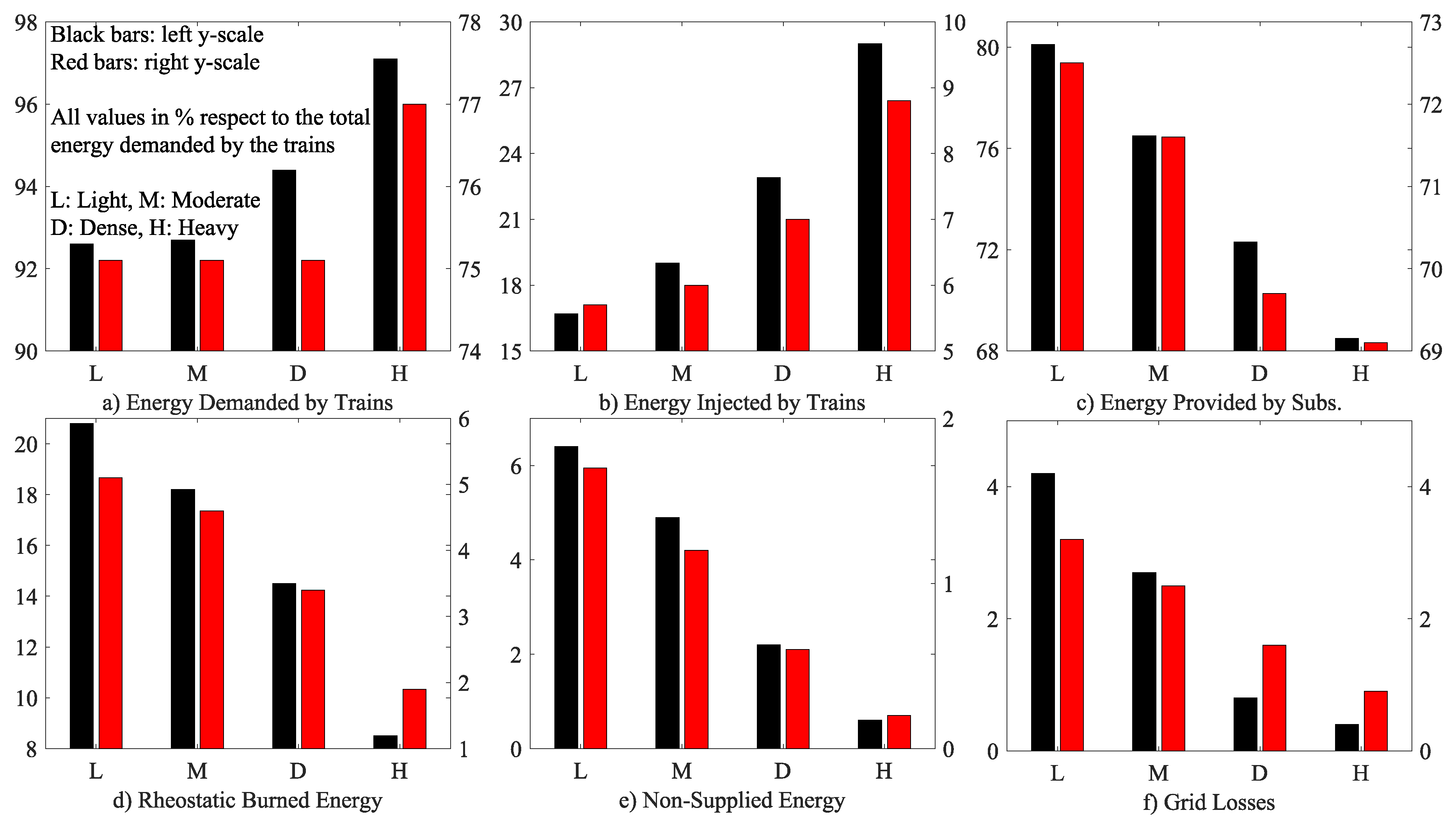
Grid Losses	4.2	3.2	2.7	2.5	0.8	1.6	0.4	0.9

. The authors are fully aware that this second table is redundant, but we think that it is important to analyze at the same time the data in MWh and in percentage with respect to the required electrical energy. The train demand in the scenario L0 was 92.6% of the required electrical energy, which means that 6.4% of the required energy cannot be provided. In order to distinguish the correlations between the different variables with the different traffic scenarios with and without energy storage and extract conclusions about the trends of the energy savings and consumption, the energetic data in percentage with respect to the total energy demanded by the trains are also represented in Figure 9. As can be observed, we had the same trends as the traffic increased for the cases with and without energy storage. However, even when the trend was the same, the values were very different, and it was necessary to add two different y-scales in order to compare the plots. The real energy demanded by the trains increased with the traffic, as well as the energy injected by the trains. That means that with denser traffic, the number of instants in which the overcurrent and overvoltage protections were activated was lower. We also reduced the energy provided by the substations and the grid losses when we increased the traffic.

The non-supplied energy in the case of the heavy traffic scenario without energy storage was only 0.6%. The non-supplied energy is represented in Row 9 of Table 4 and Table 5. This non-supplied energy in percentage is a good index of the network congestion, as it can be observed that the more trains in the system, the less the network congestion. In general, we can state that the installation of on-board energy storage always reduced the amount of non-supplied energy. In the worst scenario (light traffic), the non-supplied energy was reduced from 6.4–1.7% when we added storage to the trains. Row 5 represents the energy regenerated by the trains that was actually injected into the feeding system. Obviously, this energy increased with the traffic, but it was always reduced when we added energy storage to the trains. In Row 6, the trains’ net energy was obtained subtracting Row 5 (energy injected) from Row 4 (energy demanded). We can see that in the light, medium, and dense traffic scenario, the net energy was always lower when the trains were equipped with energy storage. However, the net energy was nearly the same in the scenarios H0 and H1. Row 7 represents the energy provided by the substations. It is very interesting to remark that even in the worst scenario (L0), the substations provided only 80% of the energy demanded by the trains, the rest being provided by other trains in braking mode. Again, for the light, medium, and dense traffic scenarios, the energy provided by the substations was reduced when we added the energy storage. In the heavy traffic scenario, this trend was inverted, and the energy provided by the substations was slightly higher when we added energy storage to the trains. This is because when we had many trains and they were very close to each other, it was more efficient to use the regenerated energy in other trains than the stored energy in the on-board accumulation system. This is coherent with the data obtained representing the losses in the feeding system (Row 10). In the heavy traffic scenario, the losses were higher when the trains were equipped with an energy storage system. Finally, Row 8 represents the energy burned in the rheostatic system of the train, in all cases, it suffered a significant reduction when we added the on-board accumulation system.

In

Table 6. Summary of the train behavior in the average trip for all lines and in all scenarios.

Energy Obtained from the Catenary (kWh)
Trip	L0	L1	M0	M1	D0	D1	H0	H1
S1 to S6 Red	238	183	238	183	245	183	249	186
S6 to S1 Red	243	173	243	173	245	171	251	174
S1 to S4 Blue	230	222	230	221	233	223	246	233
S4 to S1 Blue	181	145	182	146	186	146	189	149
Average trip	223	181	223	181	227	181	234	186
Energy Injected into the Catenary (kWh)
Trip	L0	L1	M0	M1	D0	D1	H0	H1
S1 to S6 Red	57	16	60	17	67	18	85	23
S6 to S1 Red	38	10	49	10	60	11	70	11
S1 to S4 Blue	9	7	13	7	28	12	34	13
S4 to S1 Blue	57	22	61	24	66	26	90	38
Average trip	40	14	46	15	55	17	70	21
Energy Burned in the Rheostatic Braking System (kWh)
Trip	L0	L1	M0	M1	D0	D1	H0	H1
S1 to S6 Red	49	12	45	11	40	8	22	4
S6 to S1 Red	64	6	52	5	42	4	31	4
S1 to S4 Blue	50	13	45	12	29	7	24	5
S4 to S1 Blue	37	18	33	16	29	14	5	5
Average trip	50	12	44	11	35	8	21	5
Non-Supplied Energy (kWh)
Trip	L0	L1	M0	M1	D0	D1	H0	H1
S1 to S6 Red	19	6	19	5	12	5	8	4
S6 to S1 Red	9	2	9	2	7	2	2	1
S1 to S4 Blue	9	4	24	5	21	4	10	2
S4 to S1 Blue	25	4	14	4	11	3	7	2
Average trip	15	4	16	4	13	3	7	2

, we can observe the trains’ average behavior in the different trips and in all scenarios, as well as the average trip considering all possible routes in all scenarios. The table is split into four blocks. In the first one, we represent the total energy obtained from the catenary. It should be noticed that the slope of the blue line was steeper than the slope in the red line. That is the reason why the energy obtained from the catenary in the outward and return journeys was so different, as well as the energy injected into the catenary. It must be noted that for the average trip, the energy obtained from the catenary increased when we increased the traffic because the voltage was more stable (within the limits), and the non-supplied energy decreased. The minimum consumption (theoretical) for the average trip defined in Table 2 was 151 kWh, and this number was obtained subtracting the electrical regeneration capacity from the required electrical energy. The best scenario in terms of average net consumption was H0 (heavy traffic without accumulation), with a net consumption of 164 kWh, only 5.8% above the theoretical consumption. Adding accumulation to the heavy traffic scenario increased the average trip net consumption by 1 kWh. In the rest of the scenarios, adding accumulation always improved the average trip net consumption. For instance, in the light traffic scenario, the net consumption for the average trip was 183 kWh without accumulation and 167 kWh with accumulation. It is very important to remark that when we considered the net consumption in the average trip for comparing with the theoretical limit, we were not considering the non-supplied energy that was quite high in the light, medium, and dense traffic scenarios without accumulation. When we added accumulation to the system, the non-supplied energy in the average trip was always lower than 2% with respect to the required electrical energy for the average trip; and in the case of heavy traffic, lower than 1%.

Table 7. Summary of the substations’ behavior in all scenarios.

Energy Injected into the DC Traction System (MWh)
Substation	L0	L1	M0	M1	D0	D1	H0	H1
S5 (Red line)	2.35	2.03	3.04	2.76	4.88	4.64	8.99	9.02
S3 (Red line)	3.14	2.83	4.22	3.93	6.77	6.54	12.2	12.7
S3 (Blue line)	2.20	2.12	3.04	2.95	5.05	4.93	9.76	9.53
Total	7.71	6.98	10.3	9.65	16.7	16.1	31.0	31.2
Energy Injected into the DC Traction System per Train Trip (kWh/trip)
Substation	L0	L1	M0	M1	D0	D1	H0	H1
S5 (Red line)	59	51	54	49	51	48	48	48
S3 (Red line)	79	71	75	70	71	68	65	68
S3 (Blue line)	55	53	54	53	53	51	52	51
Total	193	175	184	172	174	168	165	166
Energy Injected into the DC Traction System per Train Trip
above the Minimum Theoretical Consumption in %
	L0	L1	M0	M1	D0	D1	H0	H1
	27.8	15.8	22.1	14.3	15.3	11.3	9.3	10.3

contains the energy analysis of the substations for all scenarios; it is split into three blocks. The first block represents the energy injected into the DC traction system per each substation and the total. In the second block, we can observe the energy injected by each substation per train trip. Finally, this number is compared with the minimum theoretical consumption in Block 3. Again, we can observe that in the scenario H0, the total energy injected into all substations was only 9.3% above the minimum consumption.

Regarding the performance, both models (decoupled and integral) were equivalent from the point of view of the equations, and they provided the same result. However, the time savings on average when simulating the proposed decoupled model were around 20%. On average, the number of iterations of the decoupled model compared to the integral one was higher, from 6.5 iterations (average) to 7.9 iterations (average) per instant. The iterations using the decoupled model were faster. The average time to complete an iteration with the decoupled model was 0.39 ms, while the integral model spent 0.55 ms.

4. Conclusions

A simplified model of a storage system for power flow purposes was presented and tested. The proposed approach considered the train and the accumulation system as different devices placed at the same point of the railway traction network. Both devices were coupled and interacted with each other and with the electrical network. The proposed mathematical model reduced the computational burden of the simulation when it was compared with models that considered the train and the storage in an integral way. The model was embedded in a power flow solver, and extensive results were provided.

Analyzing the results obtained, it can be stated that the behavior of the system when adding this kind of technology cannot be easily predicted. It has been observed how reducing the train headset and increasing the traffic in the system, the non-supplied energy was reduced, as well as the number of instants at which all substations were blocked. In general, we could state that adding on-board accumulation systems to the trains reduced the burned energy in the rheostatic braking system due to the squeeze control activation and also the non-supplied power. However, this effect was highly correlated with the train headset. In order to perform comparisons with different traffic levels, all the energetic data must be normalized using as a rated value the total energy demanded by all trains in each specific scenario. In the cases studied in this work, we observed how the congestion in the network was inversely correlated with the traffic. That means that increasing the traffic, we alleviated the network, and the voltage profile was lower, so the activation of the overvoltage protection was less frequent. We observed also that with the heavy traffic scenario, the trains were able to absorb nearly 98% of the demanded energy when the on-board accumulation was installed and 77% without accumulation. The energy regenerated reached nearly 30% in the heavy traffic scenario with accumulation, when in the same situation without accumulation, it was only 9%, half of the injected regenerated power in the light traffic scenario with accumulation. As a general conclusion, it could be stated that up to a reasonable level, the increasing the traffic can alleviate the system, making it more efficient in relative terms. However, each specific infrastructure can have different behaviors, and it is important to make these kinds of studies during the infrastructure planning stage in order to make the correct decisions.

References

1. Jabr, R.A.; Dzafic, I. Solution of DC Railway Traction Power Flow Systems including Limited Network Receptivity. IEEE Trans. Power Syst. 2017. [Google Scholar] [CrossRef]
2. Arboleya, P.; Mohamed, B.; Gonzalez-Moran, C.; El-Sayed, I. BFS Algorithm for Voltage-Constrained Meshed DC Traction Networks With Nonsmooth Voltage-Dependent Loads and Generators. Power Syst. IEEE Trans. 2016, 31, 1526–1536. [Google Scholar] [CrossRef]
3. Takagi, R.; Amano, T. Optimisation of reference state-of-charge curves for the feed-forward charge/discharge control of energy storage systems on-board DC electric railway vehicles. IET Electrical Syst. Transp. 2015, 5, 33–42. [Google Scholar] [CrossRef]
4. Abrahamsson, L.; Söder, L. Fast Estimation of Relations Between Aggregated Train Power System Data and Traffic Performance. Veh. Technol. IEEE Trans. 2011, 60, 16–29. [Google Scholar] [CrossRef]
5. López-López, A.; Pecharromán, R.; Fernández-Cardador, A.; Cucala, A. Smart traffic-scenario compressor for the efficient electrical simulation of mass transit systems. Int. J. Electrical Power Energy Syst. 2017, 88, 150–163. [Google Scholar] [CrossRef]
6. Mayet, C.; Horrein, L.; Bouscayrol, A.; Delarue, P.; Verhille, J.N.; Chattot, E.; Lemaire-Semail, B. Comparison of Different Models and Simulation Approaches for the Energetic Study of a Subway. Veh. Technol. IEEE Trans. 2014, 63, 556–565. [Google Scholar] [CrossRef]
7. Mayet, C.; Delarue, P.; Bouscayrol, A.; Chattot, E.; Verhille, J.N. Comparison of Different EMR-Based Models of Traction Power Substations for Energetic Studies of Subway Lines. IEEE Trans. Veh. Technol. 2016, 65, 1021–1029. [Google Scholar] [CrossRef]
8. Mayet, C.; Bouscayrol, A.; Delarue, P.; Chattot, E.; Verhille, J.N. Electrokinematical Simulation for Flexible Energetic Studies of Railway Systems. IEEE Trans. Ind. Electron. 2018, 65, 3592–3600. [Google Scholar] [CrossRef]
9. Mayet, C.; Delarue, P.; Bouscayrol, A.; Chattot, E. Hardware-In-the-Loop Simulation of Traction Power Supply for Power Flows Analysis of Multitrain Subway Lines. IEEE Trans. Veh. Technol. 2017, 66, 5564–5571. [Google Scholar] [CrossRef]
10. Li, Q.; Wang, T.; Dai, C.; Chen, W.; Ma, L. Power Management Strategy Based on Adaptive Droop Control for a Fuel Cell-Battery-Supercapacitor Hybrid Tramway. IEEE Trans. Veh. Technol. 2018, 67, 5658–5670. [Google Scholar] [CrossRef]
11. Mohamed, B.; Arboleya, P.; González-Morán, C. Modified Current Injection Method for Power Flow Analysis in Heavy-Meshed DC Railway Networks With Nonreversible Substations. IEEE Trans. Veh. Technol. 2017, 66, 7688–7696. [Google Scholar] [CrossRef]
12. Arboleya, P.; Mohamed, B.; El-Sayed, I. DC Railway Simulation Including Controllable Power Electronic and Energy Storage Devices. IEEE Trans. Power Syst. 2018, 33, 5319–5329. [Google Scholar] [CrossRef]
13. Gelman, V. Energy Storage That May Be Too Good to Be True: Comparison Between Wayside Storage and Reversible Thyristor Controlled Rectifiers for Heavy Rail. Veh. Technol. Mag. IEEE 2013, 8, 70–80. [Google Scholar] [CrossRef]
14. Gelman, V. Braking energy recuperation. Veh. Technol. Mag. IEEE 2009, 4, 82–89. [Google Scholar] [CrossRef]
15. Arboleya, P.; Bidaguren, P.; Armendariz, U. Energy Is On Board: Energy Storage and Other Alternatives in Modern Light Railways. Electr. Mag. IEEE 2016, 4, 30–41. [Google Scholar] [CrossRef]
16. Khodaparastan, M.; Dutta, O.; Saleh, M.; Mohamed, A.A. Modeling and Simulation of DC Electric Rail Transit Systems With Wayside Energy Storage. IEEE Trans. Veh. Technol. 2019, 68, 2218–2228. [Google Scholar] [CrossRef]
17. Liu, H.; Zhou, M.; Guo, X.; Zhang, Z.; Ning, B.; Tang, T. Timetable Optimization for Regenerative Energy Utilization in Subway Systems. IEEE Trans. Intell. Transp. Syst. 2019. [Google Scholar] [CrossRef]
18. Liu, P.; Yang, L.; Gao, Z.; Huang, Y.; Li, S.; Gao, Y. Energy-Efficient Train Timetable Optimization in the Subway System with Energy Storage Devices. IEEE Trans. Intell. Transp. Syst. 2018, 19, 3947–3963. [Google Scholar] [CrossRef]
19. Mayet, C.; Pouget, J.; Bouscayrol, A.; Lhomme, W. Influence of an Energy Storage System on the Energy Consumption of a Diesel-Electric Locomotive. Veh. Technol. IEEE Trans. 2014, 63, 1032–1040. [Google Scholar] [CrossRef]
20. De la Torre, S.; Sánchez-Racero, A.J.; Aguado, J.A.; Reyes, M.; Martínez, O. Optimal Sizing of Energy Storage for Regenerative Braking in Electric Railway Systems. IEEE Trans. Power Syst. 2015, 30, 1492–1500. [Google Scholar] [CrossRef]
21. Razik, L.; Berr, N.; Khayyamim, S.; Ponci, F.; Monti, A. REM-S–Railway Energy Management in Real Rail Operation. IEEE Trans. Veh. Technol. 2018. [Google Scholar] [CrossRef]
22. Lu, S.; Hillmansen, S.; Roberts, C. A Power-Management Strategy for Multiple-Unit Railroad Vehicles. Veh. Technol. IEEE Trans. 2011, 60, 406–420. [Google Scholar] [CrossRef]
23. Khayyam, S.; Berr, N.; Razik, L.; Fleck, M.; Ponci, F.; Monti, A. Railway System Energy Management Optimization Demonstrated at Offline and Online Case Studies. IEEE Trans. Intell. Transp. Syst. 2018, 19, 3570–3583. [Google Scholar] [CrossRef]
24. Graber, G.; Calderaro, V.; Galdi, V.; Piccolo, A.; Lamedica, R.; Ruvio, A. Techno-economic Sizing of Auxiliary-Battery-Based Substations in DC Railway Systems. IEEE Trans. Transp. Electr. 2018, 4, 616–625. [Google Scholar] [CrossRef]
25. Mohamed, B.; El-Sayed, I.; Arboleya, P. DC Railway Infrastructure Simulation Including Energy Storage and Controllable Substations. In Proceedings of the 2018 IEEE Vehicle Power and Propulsion Conference (VPPC), Chicago, IL, USA, 27–30 August 2018; pp. 1–6. [Google Scholar]
26. Gee, A.M.; Dunn, R.W. Analysis of Trackside Flywheel Energy Storage in Light Rail Systems. IEEE Trans. Veh. Technol. 2015, 64, 3858–3869. [Google Scholar] [CrossRef]
27. Alfieri, L.; Battistelli, L.; Pagano, M. Impact on railway infrastructure of wayside energy storage systems for regenerative braking management: A case study on a real Italian railway infrastructure. IET Electr. Syst. Transp. 2019. [Google Scholar] [CrossRef]
28. Arboleya, P.; Coto, M.; Gonzalez-Moran, C.; Arregui, R. On board accumulator model for power flow studies in DC traction networks. Electric Power Syst. Res. 2014, 116, 266–275. [Google Scholar] [CrossRef]
29. Gomez-Exposito, A.; Mauricio, J.; Maza-Ortega, J. VSC-based MVDC railway electrification system. IEEE Trans. Power Deliv. 2014, 29, 422–431. [Google Scholar] [CrossRef]
30. Bai, Y.; Cao, Y.; Yu, Z.; Ho, T.K.; Roberts, C.; Mao, B. Cooperative Control of Metro Trains to Minimize Net Energy Consumption. IEEE Trans. Intell. Transp. Syst. 2019. [Google Scholar] [CrossRef]
31. Kleftakis, V.A.; Hatziargyriou, N.D. Optimal control of reversible substations and wayside storage devices for voltage stabilization and energy savings in metro railway networks. IEEE Trans. Transp. Electr. 2019. [Google Scholar] [CrossRef]
32. Clerici, A.; Tironi, E.; Castelli-Dezza, F. Multiport Converters and ESS on 3-kV DC Railway Lines: Case Study for Braking Energy Savings. IEEE Trans. Ind. Appl. 2018, 54, 2740–2750. [Google Scholar] [CrossRef]
33. Zhao, J.; Gao, Y.; Guo, J.; Chu, L.; Burke, A.F. Cycle life testing of lithium batteries: The effect of load-leveling. Int. J. Electrochem. Sci 2018, 13, 1773–1786. [Google Scholar] [CrossRef]
34. Arboleya, P. Heterogeneous multiscale method for multirate railway traction systems analysis. IEEE Trans. Intell. Transp. Syst. 2017, 18, 2575–2580. [Google Scholar] [CrossRef]
Figure 1. Equivalent mathematical model of the train plus storage system (a) Traction mode. (b) Braking mode.
Energies 12 02199 g001
Figure 2. Subfigures (ac) represent the functions that model the behavior of the train and the storage in traction mode. Subfigures (df) represent the functions that model the behavior of the train and the storage in braking mode. (a) Train overcurrent protection in traction mode. (b) Maximum power that can be extracted from the storage system in traction mode as a function of the energy level. (c) Available discharging power in the storage system as a function of the voltage (overcurrent protection of the storage in traction mode). (d) Train squeeze control in braking mode. (e) Maximum power that can be injected into the storage system in braking mode as a function of the energy level. (f) Available charging power in the storage system as a function of the voltage (overcurrent protection of the storage system in braking mode).
Energies 12 02199 g002
Figure 3. Schematic representation of the case study.
Energies 12 02199 g003
Figure 4. Detailed behavior of the fourth train on the red line from S1 to S6 in the light traffic scenario with on-board energy storage. (a) Mechanical reference power; power extracted from the catenary and burned in the rheostatic system. (b) Catenary voltage. (c) Storage system power (in black) and state of charge of the energy storage system (in red) in (p.u.).
Energies 12 02199 g004
Figure 5. Detailed behavior of the fourth train on the blue line from S1 to S4 in the heavy traffic scenario with on-board energy storage. (a) Mechanical reference power; power extracted from the catenary and burned in the rheostatic system. (b) Catenary voltage. (c) Storage system power (in black) and state of charge of the energy storage system (in red) in (p.u.).
Energies 12 02199 g005
Figure 6. Power in MW obtained from the AC grid by substation S5 on the red line for all scenarios. (a) Light Traffic Scenario; (b) Medium Traffic Scenario (c) Dense Traffic Scenario; (d) Heavy Traffic Scenario.
Energies 12 02199 g006
Figure 7. Energy in MWh obtained from the AC grid by substation S5 on the red line for all scenarios.
Energies 12 02199 g007
Figure 8. Marey diagrams representing the first 80 min of the schedule of the red line in the different scenarios. Solid lines represent the trains moving from S1 to S6, while dashed-dotted lines represent the trains moving from S6 to S1. The vertical red lines mark the instants at which all the substations in the system were blocked due to the high regenerated power surplus. The number in the top-left corner of each subfigure represents the percentage of instants at which all the substations were blocked at the same time for the whole simulation interval. The scenario is indicated in the top-right corner of each subfigure. (a) Light Traffic without accumulation; (b) Medium traffic without accumulation; (c) Dense traffic without accumulation; (d) Heavy traffic without accumulation; (e) Light Traffic with accumulation; (f) Medium traffic with accumulation; (g) Dense traffic with accumulation; (h) Heavy traffic with accumulation.
Energies 12 02199 g008
Figure 9. Energy comparison of the different scenarios. In order to compare scenarios with a very different number of trains, all the energy values have been expressed in percentage referring to the total energy demanded by the trains in each scenario. This value can be found for each scenario in the first row of the Table 4. Black bars represent the cases without energy storage, and they are associated with the y-scale on the left. Red bars represent the cases with energy storage, and they are associated with the y-scale on the right.
Energies 12 02199 g009