Abstract
Affected by high density, non-uniform, and unstructured seawater environment, fault detection of Marine Current Turbine (MCT) faces various fault features and strong interferences. To solve these problems, a harmonic analysis strategy based on zero-crossing estimation and Empirical Mode Decomposition (EMD) filter banks is proposed. First, the detection problems of rotor imbalance fault under strong interference conditions are described through an analysis of the fault mechanism and operation environment of MCT. Therefore, against various fault features, a zero-crossing estimation is proposed to calculate instantaneous frequency. Last, and in order to solve the problem that the frequency and amplitude of the operating parameters are partially or completely covered by interference, a band-pass filter based on EMD is used, together with a characteristic frequency selected by a Pearson correlation coefficient. This strategy can accurately detect the multiplicative faults under strong interference conditions, and can be applied to the MCT fault detection system. Theoretical and experimental results verify the effectiveness of the proposed strategy.
1. Introduction
Timely maintenance can prolong the life of an MCT. Condition-based maintenance technology is a pivotal solution to reduce the long-term operation and maintenance cost of MCTs [1]. However, due to the complex marine environment, the condition-based maintenance of MCT faces the following problems: few monitoring variables, various fault features, and strong interferences [2]. In order to improve the safety and reliability of MCT, a fault detection strategy for non-stationary signals with strong interference is needed [3].
Condition monitoring provides continuous indications of components based on techniques, including vibration analysis, temperature, and acoustic emission analysis, among others [3]. Because of the limitations of underwater environment sensors, fault detection based on stator current has several advantages, since it is a non-invasive technique and avoids the use of additional sensors [4]. Regarding current-based detection methods, fault causes can be divided into two types: additive and multiplicative faults. Additive faults refer to the superposition of a pulse signal, a constant signal or a random small signal on the original normal signal [5], while multiplicative faults refer to signals with a certain frequency superimposed on the original normal signal [6]. For additive fault detection, time-domain statistical analysis can be used. A recursive principal component method can be applied to update the control limit adaptively to detect motor faults under unstable working conditions [7]. Multiplicative faults should be rather detected on the basis of energy frequency characteristics. Under stable working conditions, detections can be completed by frequency domain analysis. However, the magnitude of different frequency components changes with working conditions in practice [8]. Therefore, frequency domain analysis can be used in such conditions. Local feature detection, such as Short-Time Fourier Transforms (STFT) [9], Wavelet Transforms (WT) [10], and Hilbert-Huang transforms [11], can then be applied. STFT is used in [12] for blade crack detection of wind turbine to identify time-varying fault frequencies. In [13], motor current signature analysis is applied based on two sets of over complete wavelets; the gear fault-related component is highlighted under different operating conditions. In [14], SVD filtering combines the parameter estimation technique of rotation invariant signal to detect broken rotor bars under variable operating conditions. However, these methods identify the characteristic frequency, which amplitudes are very low in practice, and therefore may be partially or completely covered by the fundamental frequency and strong interference.
In order to solve these problems, we introduce a harmonic analysis strategy based on zero-crossing estimation and EMD filter banks. First, the detection problems of rotor imbalance fault under strong interference conditions are described through an analysis of the fault mechanism and operation environment of MCT. Therefore, against various fault features, zero-crossing estimation is proposed to calculate the instantaneous frequency. In order to solve the problem that the frequency and amplitude of the operating parameters are partially or completely covered by interference, a band-pass filter based on EMD is applied. Next characteristic frequency is selected by a Pearson correlation coefficient. Overall, this method can improve the detection accuracy of multiplicative faults, and has practical significance for ensuring the safe operation of MCT. The rest of the paper is organized as follows. Section 2 introduces the problem description, while Section 3 develops a harmonic analysis strategy. Section 4 presents some simulation results and analysis. Section 5 presents some experimental results and analysis, while Section 6 concludes the paper and draws perspectives for further work.
2. Problem Description
A MCT system harnesses energy from tidal flow, which converts kinetic energy into the motion of a turbine and then drives electrical generators. In comparison with wind turbines, MCTs have high energy density and small moment of inertia. Influenced by the tide, long-term flow velocity varies in a wide range, and short-term flow velocity varies frequently [15]. Waves, turbulence, and watershed topography are main interference factors affecting MCT working conditions [16]. For MCT multiplication faults, taking blade imbalance fault as an example, specific frequencies can be detected in stator current. However, affected by interference, the monitoring signal has multiple time scales and multiple characteristics [17]. This seriously affects the accuracy of fault detection.
2.1. Multiplication Fault of MCT
This section mainly describes the multiplicative faults of MCT under strong interference. Take blade imbalance fault as an example; this fault refers to the signal with a certain 1P frequency superimposed on the original normal stator current signal.
The kinetic energy harnessed by the turbine can be described as:
where is power coefficient, the water density, the cross-sectional area of the turbine, the tidal current velocity, and is mechanical torque and speed. The turbine drives an electrical generator. Considering the generator as a permanent magnet synchronous motor, the motion equation is given as:
where is the moment of inertia, friction coefficient, electromagnetic torque. The current output can described as:
where is the amplitude of the stator current, the number of pole pairs. The relationship between these variables is shown in Figure 1.
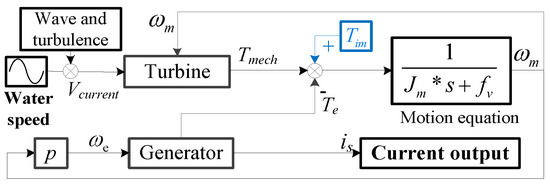
Figure 1.
Energy transfer mechanism of MCT.
When imbalance fault happens, additional torque appears as shown in Figure 1. Mechanical speed accelerates when imbalance mass falls in the direction of rotation, and mechanical speed decelerates when imbalance mass goes upward in the direction of reverse rotation, as shown in Figure 2.
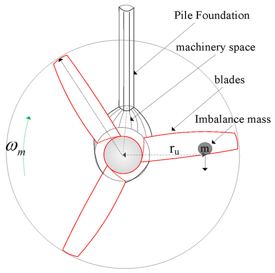
Figure 2.
Effect of imbalance mass on the MCT.
Additional torque caused by imbalance fault can be described as:
where is resultant of forces downward, is the distance between attachments to the center of the shaft. Bring additional torque into Equation (2), then additional speed can be obtained as:
Considering , the stator current can be expressed as:
where is the initial angle. In this case, stator current frequency is , the fault feature frequency is .
2.2. The Effect of Strong Interference
With a changeable water speed, mechanical torque can be written as:
where stands for slowly time-varying torque, stands for abrupt change torque. The torque is caused by long-term tidal velocity, as shown in Figure 3. It provides one month water flow velocity variation curve—the velocity changes in a large range. The torque is caused by spatial velocity change, as shown in Figure 4. changes frequently due to unstable flow velocity, which results in strong interference.
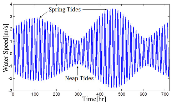
Figure 3.
Long-term tidal velocity.
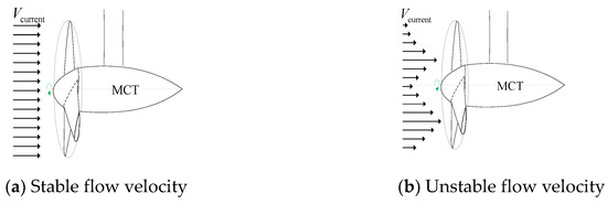
Figure 4.
Spatial velocity change.
Combining Equations (7) and (2), mechanical speed can be rewritten as:
Accordingly, stands for slowly time-varying rotating speed. stands for abrupt change rotating speed. The strong interference factor is taken into the calculation of stator current in Equation (6), which can be rewritten as:
The fault feature frequency changes with the mechanical cycle; may be partially or completely covered by interference frequency .
Figure 5 shows the mechanical phases in three cases: constant rotating speed, slowly time-varying rotating speed, and abrupt change rotating speed. In Figure 5a, imbalance faults can be accurately distinguished. However, when the rotating speed changes slowly, the imbalance fault feature frequency changes as shown in Figure 5b. When the rotating speed changes frequently, imbalance fault are not able to detect, features are partially or completely covered by interference, as shown in Figure 5c.
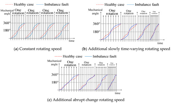
Figure 5.
Mechanical phase affected by interference.
3. Proposed Harmonic Analysis Strategy
This section aims to solve the fault feature extraction problem under the condition of variable speed operation and strong disturbance. Fault feature has many different possible forms under strong interference conditions. The proposed detection method consists of three parts: The zero-crossing estimation is used to unify characteristic frequency; the interference signal is decomposed to several intrinsic mode functions by EMD filter banks; the specific data for extracting the characteristic frequency is selected by Pearson correlation coefficient.
3.1. Instantanous Frequency Caculation by Zero-Crossing Estimation
The fault feature has many different possible forms. If the original stator current signal is uniformly sampled with sampling frequency, Equation (6) can be rewritten as:
Find all zero-crossing pairs . If () then (). Using linear interpolation for each zero-crossing point of the sequence, we can get the time value of the zero-crossing point:
where is the time of , is the time of . The total number of sampling points in each mechanical cycle is variable because of the changing shaft rotating speed. Assume are the zero-crossing points for one mechanical cycle, (Z is determined by the number of generator poles). The instantaneous frequency defined at is:
where ,,. Then, cubic spline interpolation is used to obtain the instantaneous frequency curve.
For the mechanical cycle, the time span is to . Each mechanical cycle is different taking into account the effect of rotational speeds. The average time of mechanical cycle can be denoted as There are two major parts to unify the fault feature form:
1). Scaling on the Time Axis
In order to unify fault feature frequency, set up the total time of each mechanical cycle , then the time for each zero-crossing point is changed to:
By Equation (13), we reconstruct a time series, and a unified characteristic frequency can be the obtained.
2). Eliminate the Trend Component
As shown in Figure 6, Least Square (LS) is used to eliminate the trend component according to the size of the windows. Different fluctuation curve is retained to highlight the fault degree. For 1P frequency, the length of window is selected as . After LS, the fluctuation curve of instantaneous frequency is obtained.
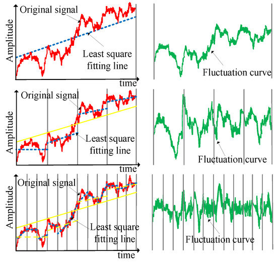
Figure 6.
LS with different size of windows.
3.2. Interference Filtering by EMD Filter Banks
In order to effectively remove the influence of strong interference, an EMD-based filter bank is proposed. The aim of this method is to extract the characteristic frequency signal from the original dataset. Affected by interference, the amplitude of characteristic frequency cannot be accurately obtained. EMD-based filter bank decomposes the interference signal into several intrinsic mode functions to reduce the influence of interference on characteristic frequency signals. Sampling frequency is then set up. From Equation (5), the frequency variation affected by interference can be obtained:
In consideration of , can be approximated as zero; Equation (14) can be rewritten as:
where is the noise component caused by strong interference. Equation (15) is expressed as the sum of characteristic frequency components and noise components, which can be composed of a set of intrinsic mode functions (IMFs) and residual terms:
where , is residual term, is used to indicate IMFs, can be represented as:
where is the average value of the upper envelope and the lower envelope, is maximum number of iterations to calculate the intrinsic mode function. Average trend of the signal is:
If there is no interference, . The average value of the upper envelope and the lower envelope become zero. Fault feature frequency is obtained in . EMD can make tending to the null value; the interference components are distributed into different IMFs.
3.3. Characteristic Frequency Selection by Pearson Correlation Coefficient
The Pearson correlation coefficient is used to determine which IMF contains fault feature frequency. With and two-time series, Pearson correlation coefficient is defined as:
where and is the average value. The value of is from −1 to 1; −1 indicates negative correlation, 1 indicates positive correlation, and 0 irrelevant. Assume that and , because only one contains characteristic frequency and the other contains the noise component; the largest is selected to realize EMD filtering.
3.4. Harmonic Analysis Strategy for Fault Detection
The procedure of harmonic analysis strategy for multiplier fault under strong interference is shown in Figure 7. The details are as follows:
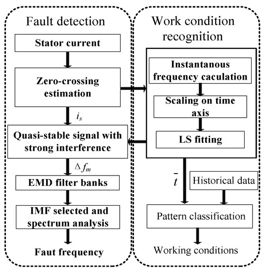
Figure 7.
Flow chart of the proposed method.
- (1)
- Measuring the current signal from MCT.
- (2)
- Zero-crossing estimation is used to calculate the instantaneous frequency by Equation (12). Then, a unified characteristic frequency is obtained by reconstructing the time series, and the LS method is used to eliminate the trend component. By combining historical data, the estimated instantaneous frequency is used to identify the work conditions of MCTs.
- (3)
- To solve the problem that the frequency and amplitude of the operating parameters are partially or completely covered by interference, an EMD filter bank is used to remove interference in the frequency band.
- (4)
- The IMF selected by Pearson correlation coefficient is analyzed by spectrum analysis, which provides fault feature frequency.
4. Simulation Results and Analysis
A sample example is given to illustrate the effectiveness of the proposed method. An AM/FM signal is given as:
Signal fundamental frequency is 16 Hz, FM frequency 2 Hz, high-order FM frequency 80 Hz, AM frequency 2 Hz. The instantaneous frequency of the modulated signal is then obtained:
Figure 8 shows the time-frequency spectrum used by Hilbert transform and separately proposed the zero-crossing estimation method. From Figure 8a, Hilbert transform can present high-order harmonics. However, the boundary effects affect estimation accuracy. Figure 8b shows the FM frequency 2 Hz more clearly and gets rid of the high frequency harmonics by scaling the time axis and Equation (13). The time span in Figure 8a is different from Figure 8b due to time axis expansion and contraction. In Equation (12), , . The proposed zero-crossing estimation method realizes purposeful fault feature frequency extraction, and overcomes shortcomings of the Hilbert transform.
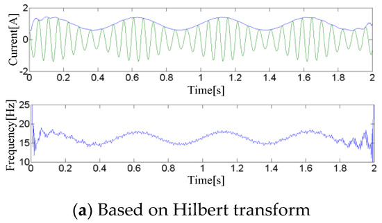
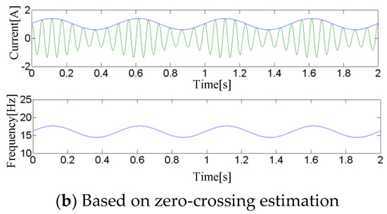
Figure 8.
Simulation test result of time-frequency spectrum.
5. Experimental Results and Analysis
5.1. MCT Experiment and Analysis
In order to verify the proposed method, a MCT prototype is implemented in an experimental platform, as shown in Figure 9. This experiment platform consists of the following parts: (1) current simulation system (enclosed water channel: adjustable flow velocity 0.2m/s‒1.5m/s); (2) MCT prototype (PMSG: 8 pole-pairs); (3) data acquisition and monitoring system (sampling frequency 1 kHz); (4) imbalance fault setting, as shown in Figure 10.
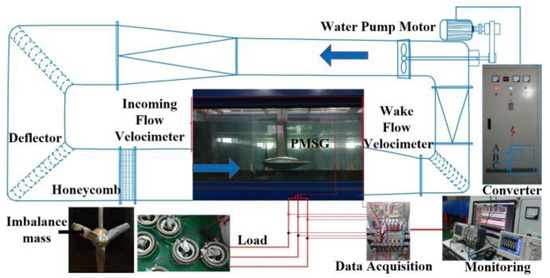
Figure 9.
MCT experimental system.
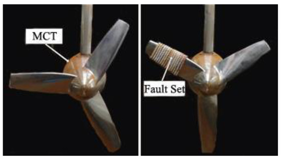
Figure 10.
Imbalance fault setting.
Figure 11 shows the stator current of MCT under a strong interference working condition [18]. One can note that when the velocity changes frequently, the collected waveforms fluctuate sharply. Under the condition of abrupt change flow velocity, both the original signal and the instantaneous frequency vary frequently with the change of flow velocity. The fault feature frequency is partially or completely covered by interference. The experimental phenomena coincide with the theoretical analysis, as shown in Equation (9).
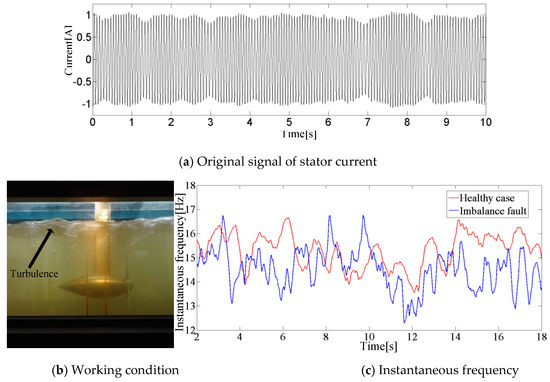
Figure 11.
MCT strong interference working condition.
5.2. Fault Detection and Analysis
The proposed method is used to detect faults in two cases: the normal operation of the MCT and 3% imbalanced faults. The magnitude ratio of the imbalanced torque to the total mechanical torque of the MCT is used to describe the degree of the faults.
Figure 12 shows the detection results after an EMD-based filter bank. The original signal is decomposed into IMF1-IMF8. Noise or interference with similar frequencies is distributed to the same IMF, which can highlight fault feature frequency. After separating the interference component, the amplitude of characteristic frequency obtained is more accurate; this can help identify the fault degree. In Figure 12a, the maximum value of is 0.104 to IMF2. In Figure 12b, the maximum value of is 0.973 to IMF2.
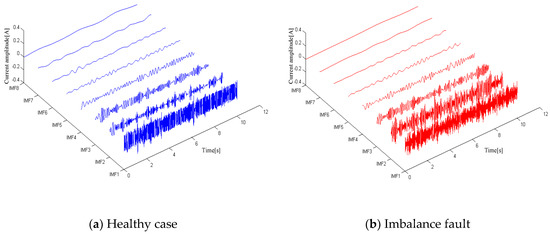
Figure 12.
Decomposition results of an EMD-based filter bank.
In Figure 13, it can be seen that the spectrum appears near the frequency of 1.875 Hz in IMF2, which corresponds to the characteristic frequency (1P frequency) of the imbalanced fault of MCT system. Several frequency components generated by strong interference are distributed on different IMFs by EMD, which greatly reduces the influence of interference and highlights the fault feature frequency.
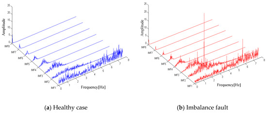
Figure 13.
Proposed detection result under strong interference conditions.
Figure 14 is the front panel of the block diagram program designed by LABVIEW. The proposed strategy is used in this monitoring system. The detection result of the MCT system is given, including short-term original signal, time-frequency spectrum, frequency difference by LS method and fault feature frequency. The last is the spectrum diagram of IMF, which has maximum value of . The input signal of the monitoring system is the stator current, and the output of the system is the working condition of the MCT and fault condition. The experimental results show that the proposed method can effectively eliminate strong interference and solve the problem that the frequency and amplitude of the operating parameters are partially or completely covered by interference.
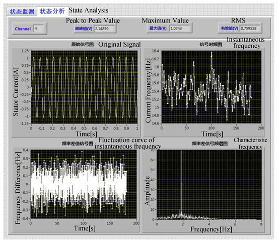
Figure 14.
Detection results of the monitoring system.
6. Conclusions
A MCT fault detection method based on zero-crossing estimation and EMD-based filter bank is proposed to deal with strong interference conditions. This method can identify working conditions by scaling on time axis and the LS fitting method. EMD is used to realize the function of filter banks by distributing the interference frequency in different IMFs. Last, Pearson correlation coefficient is used to determine which IMF contains fault characteristics frequency. The following conclusions are drawn:
(1) Zero-crossing estimation can identify specific frequencies purposefully, and effectively identify working conditions. On combining with EMD-based filter banks, the proposed method can effectively solve the problem that the frequency and amplitude of operating parameters are partially or completely covered under strong interference.
(2) Zero-crossing estimation can be easily implemented in the monitoring system, compared to STFT and WT. This method has good performance to estimate instantaneous frequency and can be used for long-term monitoring of current machine systems. However, this method has a low frequency resolution, not suitable for short-time signal processing.
It is worth pointing out that the real marine environment is more disturbing than what we simulate [19]. Due to wave, turbulence, and marine organisms, monitoring signals exhibit unstable, non-linear and low signal-to-noise ratio characteristics [20]. The proposed method may be more needed in these harsh environments.
Author Contributions
Conceptualization, M.Z.; methodology, M.Z.; software, Z.L.; validation, M.Z.; formal analysis, M.Z.; investigation, M.Z., Z.L.; resources, M.Z., T.T.; writing—original draft preparation, M.Z.; writing—review and editing, C.C.; visualization, C.C.; supervision, T.T.; project administration, T.T.; funding acquisition, T.W.
Funding
This paper is supported by the National Natural Science Foundation of China (61673260) and Shanghai Natural Science Foundation (16ZR1414300).
Conflicts of Interest
The authors declare no conflict of interest.
References
- Besnard, F.; Bertling, L. An Approach for Condition-Based Maintenance Optimization Applied to Wind Turbine Blades. IEEE Trans. Sustain. Energy 2010, 1, 77–83. [Google Scholar] [CrossRef]
- Zhang, M.; Wang, T.; Tang, T.; Benbouzid, M.; Diallo, D. An imbalance fault detection method based on data normalization and EMD for marine current turbines. ISA Trans. 2017, 68, 302–312. [Google Scholar] [CrossRef]
- Márquez, F.P.G.; Tobias, A.M.; Pérez, J.M.P.; Papaelias, M. Condition monitoring of wind turbines: Techniques and methods. Renew. Energy 2012, 4, 169–178. [Google Scholar] [CrossRef]
- Feng, Z.; Chen, X.; Zuo, M.J. Induction Motor Stator Current AM-FM Model and Demodulation Analysis for Planetary Gearbox Fault Diagnosis. IEEE Trans. Ind. Inform. 2018, 15, 2386–2394. [Google Scholar] [CrossRef]
- Tellili, A.; ElGhoul, A.; Abdelkrim, M.N. Additive fault tolerant control of nonlinear singularly perturbed systems against actuator fault. J. Electr. Eng. 2017, 68, 68–73. [Google Scholar] [CrossRef]
- Tan, C.P.; Edwards, C. Multiplicative fault reconstruction using sliding mode observers. In Proceedings of the 2004 5th Asian Control Conference, Melbourne, Australia, 20–23 July 2004; Volume 2, pp. 957–962. [Google Scholar]
- Yu, T.; Wang, X.; Shami, A. Recursive Principal Component Analysis-Based Data Outlier Detection and Sensor Data Aggregation in IoT Systems. IEEE Internet Things J. 2017, 4, 2207–2216. [Google Scholar] [CrossRef]
- Elghali, S.E.B.; Benbouzid, M.E.H.; Charpentier, J.F. Marine Tidal Current Electric Power Generation Technology: State of the Art and Current Status. In Proceedings of the 2007 IEEE International Electric Machines & Drives Conference, Antalya, Turkey, 3–5 May 2007; Volume 2, pp. 1407–1412. [Google Scholar]
- Satpathi, K.; Yeap, Y.M.; Ukil, A.; Geddada, N. Short-Time Fourier Transform Based Transient Analysis of VSC Interfaced Point-to-Point DC System. IEEE Trans. Ind. Electron. 2018, 65, 4080–4091. [Google Scholar] [CrossRef]
- Zhang, L.; Lang, Z.-Q. Wavelet Energy Transmissibility Function and Its Application to Wind Turbine Bearing Condition Monitoring. IEEE Trans. Sustain. Energy 2018, 9, 1833–1843. [Google Scholar] [CrossRef]
- Koganezawa, S. Frequency analysis of disturbance torque exerted on a carriage arm in hard disk drives using Hilbert-Huang Transform. IEEE Trans. Magn. 2018, 99, 1–6. [Google Scholar] [CrossRef]
- Jian-Zhong, W.U.; Yi, T. STFT-based crack detection on wind turbine blades. Chin. J. Constr. Mach. 2014, 12, 180–183. [Google Scholar]
- Chai, N.; Yang, M.; Ni, Q.; Xu, D. Gear fault diagnosis based on dual parameter optimized resonance-based sparse signal decomposition of motor current. IEEE Trans. Ind. Appl. 2018, 54, 3782–3792. [Google Scholar] [CrossRef]
- Brenner, M.J. Non-Stationary Dynamics Data Analysis with Wavelet-Svd Filtering. Mech. Syst. Signal Process. 2001, 17, 765–786. [Google Scholar] [CrossRef][Green Version]
- Zhang, M.; Wang, T.; Tang, T.; Benbouzid, M.; Diallo, D. Imbalance fault detection of marine current turbine under condition of wave and turbulence. In Proceedings of the IECON 2016—42nd Annual Conference of the IEEE Industrial Electronics Society, Florence, Italy, 24–27 October 2016; pp. 6353–6358. [Google Scholar]
- Zhang, M.; Wang, T.; Tang, T.; Wang, Y. Blade Imbalance Fault Detection Method for Direct-Driven Marine Current Turbine with Permanent Magnet Synchronous Generator. Trans. China Electrotech. Soc. 2018, 33, 38–47. [Google Scholar]
- Samantaray, L.; Dash, M.; Panda, R. A Review on Time-frequency, Time-scale and Scale-frequency Domain Signal Analysis. IETE J. Res. 2005, 51, 287–293. [Google Scholar] [CrossRef]
- Lust, E.E.; Luznik, L.; Flack, K.A.; Walker, J.M.; Van Benthem, M.C. The influence of surface gravity waves on marine current turbine performance. Int. J. Mar. Energy 2013, 3, 27–40. [Google Scholar] [CrossRef]
- Thomson, J.; Polagye, B.; Durgesh, V.; Richmond, M.C. Measurements of Turbulence at Two Tidal Energy Sites in Puget Sound, WA. IEEE J. Ocean. Eng. 2012, 37, 363–374. [Google Scholar] [CrossRef]
- Keenan, G.; Sparling, C.; Williams, H.; Fortune, F.; Davison, A. SeaGen Environmental Monitoring Programme: Final Report; Royal Haskoning Enhancing Society: Amersfoort, The Netherlands, 2011. [Google Scholar]
© 2019 by the authors. Licensee MDPI, Basel, Switzerland. This article is an open access article distributed under the terms and conditions of the Creative Commons Attribution (CC BY) license (http://creativecommons.org/licenses/by/4.0/).