Research on Optimization Allocation Scheme of Initial Carbon Emission Quota from the Perspective of Welfare Effect

Abstract

The initial allocation of carbon emission quotas should be of primary concern when establishing China’s unified carbon emission trading market. Essentially, the issue of national carbon quota allocation is an allocation among China’s provinces. The novel bi-level allocation scheme that is based on weighted voting model is put forward, which divides allocation process into two levels, given that there are great regional differences in China. At the first level, k-means clustering is employed to cluster 29 provinces into four categories that are based on emission abatement responsibility, potential, capacity, pressure, and motivation. Subsequently, the national carbon quotas are allocated to the four classes. At the second level, carbon quotas of a class are allocated to each region in this class. The weighted voting models are constructed for the two levels, where each region selects their preferable scheme from three fundamental allocation schemes that are based on their voting rights. The comprehensive index method quantifies each region’s voting rights, which utilizes the information entropy method at the first level and the analytic hierarchy process (AHP) at the second level. The carbon trading market is simulated and welfare effects obtained from carbon trading market under different allocation schemes are measured to verify the rationality of the proposed model. The results indicate: (1) the emission abatement burdens are borne by all provinces in China, but the burden shares are different, which are related to their respective carbon emission characteristics. (2) The differences in carbon intensity among regions in 2030 have narrowed on the basis of the results of 2005, which means that the proposed scheme can balance corresponding differences. (3) When compared with three fundamental allocation schemes, the bi-level allocation scheme can obtain the most welfare effects, while the differences in the welfare effect among regions under this scheme are the smallest, which indicates that the proposed model is feasible for policy-maker.

1. Introduction

Global surface temperatures and sea levels are expected to increase by 4.8 °C and 0.82 m by 2100, respectively, due to greenhouse effect [1]. CO₂ is one of the main greenhouse gases, and its excessive emissions have attracted massive attention with the rapid development of the world economy. China is faced with great pressure in reducing emission and addressing global warming, as the largest energy consumer and CO₂ emitter in the world [2]. Under the circumstance, a series of emission mitigation targets have been put forward. At the Copenhagen conference, China’s government promised that CO₂ emissions per unit GDP, namely, carbon intensity, are reduced by 40–45% by 2020 based on the 2005 level, which was listed in the 12th Five-Year Plan [3]. Additionally, China committed to achieving peak CO₂ emissions no later than 2030 [4] and lower carbon intensity by 60–65% by 2030 at the Paris Climate Conference [5]. China is actively taking measures, such as developing renewable energy, adjusting energy structure [6], and establishing carbon trading market to achieve the above emission reduction commitments. Recently, a nationwide carbon trading market was launched at the end of 2017 [7]. However, this market is still in the experimental stage, and there are still many problems to be solved [8], such as initial allocation of carbon emission quota. The initial allocation of quota is the most significant part and it should be of primary concern when designing the carbon trading market, as it plays a fundamental role in determining reduction responsibility. In addition, this issue directly affects the cost of carbon trading [9] and the implementation efficiency of emission abatement policies. Essentially, the issue of national carbon quota allocation is the allocation among China’s provinces. Therefore, this paper aims to study quotas allocation across provinces in China.

Carbon emission quotas determine emission mitigation responsibility for each emission unit, urging them to formulate more feasible and effective emission abatement schemes. Numerous literatures discussed the allocation scheme of carbon emission quotas in a different level, which can be grouped into two types based on their research level, namely, the international level and interregional level.

At the international level, there is currently no consensus on how to distribute the global carbon quota between the developed and developing countries. To solve the problem, researchers have put forward various allocation schemes that are based on different considerations. Shuai et al. [10] combined the STIRPAT model with the panel and time-series data to analyze the impacts of population, affluence, and technology on the carbon emission of 125 countries at different income levels over the period of 1990–2011. Pang et al. [11] employed the ZSG-DEA model to reallocate carbon quotas in order to make all countries obtain 100% efficiencies and Pareto improvement, which only took the efficiency principle into account, while ignoring the principle of equity. Similarly, Chiu et al. [12] used the ZSG-DEA model to explore the allocation and reallocation of emission quota among 24 European Union (EU) countries. Pan et al. [13] proposed an allocation scheme according to cumulative carbon emission per capita in order to achieve a globally fair carbon emission. When compared to other allocation schemes, this scheme simultaneously considered the historical emissions and future needs of developed and developing countries. 20 key allocation schemes of the equity-efficiency tradeoff side were extensively compared using the Equitable Access to Sustainable Development model in [14,15]. Ciscar et al. [16] used the multi-sector computable general equilibrium (CGE) model of the global economy to compare a perfect carbon market without transaction costs with the case of a gradually developing carbon market, i.e., a carbon market with (gradually diminishing) transaction costs.

Different from the carbon quota allocation in international level, the allocation policy is comparatively easy to formulate at the interregional level due to a stronger legislative and law enforcement capabilities of the central government. Thus, a more detailed quota allocation scheme can be designed. Since 2005, the developed countries have implemented carbon emission trading schemes [17], such as United Kingdom (UK) Emissions Trading Group (ETG) and Chicago Climate Exchange (CCX) [18,19], possessing more theoretical knowledge and practical experience. Zetterberg employed [20] economic analysis to assess the grandfathering, auctioning, and benchmarking approaches for carbon quota allocation and then discuss practical experience from American schemes. Zhou et al. [21] analyzed the potential profit impacts and possible compensation to generation companies through modeling the Australian Electricity Market under a carbon quota trading scheme to study the optimal ratio of free quota allocation. Hong et al. [22] aimed to develop a decision support model as a tool for quota allocation in the construction industry of South Korea. Edwards et al. [23] employed a CGE model to evaluate various quota allocation methods among twelve sectors within UK.

Unlike the developed countries, a vast regional and sectorial difference in economic development and energy structure in China exists. Thus, it is particularly complex for China to allocate the carbon quota. Numerous researches aimed to put forward policy suggestions or impact analysis in terms of China’s quota allocation. The DEA model is generally utilized in the evaluation of efficiency [24]. Wang et al. [25] employed the DEA to evaluate the carbon emission efficiency of 30 provinces in China. In the meantime, it also proves to be a feasible approach in allocating the emission quotas from the perspective of efficiency. Zhang and Hao [26] applied an input-oriented ZSG-DEA model to allocate the carbon quota among China’s 39 industrial sectors in 2020. Similar studies assigning carbon quotas from the efficiency perspective include Feng et al. [27], Ji et al. [28], and An et al. [29]. Zhou et al. [8] compared the five indicators of carbon emissions, energy consumption, GDP, population, and per capita GDP, and found population and historical carbon emissions seem to be fairer than other indicators to reflect the equality principle. Han et al. [9] built a comprehensive index to allocate carbon quotas in the Beijing-Tianjin-Hebei region. The Boltzmann distribution was exploited in the allocation of carbon emission quotas among enterprises [30] and power plants [31]. The clustering methods that were discussed in [32,33] selected five indicators to cluster 30 China’s province, respectively, but they both did not consider the historical emission, technical level, and urbanization level. Yang et al. [34] put forward an allocation scheme according to the gradual efficiency improvement and emission abatement principles, which ignored equity. Three indicators, namely, emission abatement capacity, responsibility, and potential, were chosen to assess equity and efficiency of each emission unit [35,36], in which accumulated carbon emissions were used to reflect the emission reduction responsibility without taking demographic factors and the current emissions into account.

The above researches mainly pay attention to single scheme in carbon quota allocation, which cannot reflect the preference of each emission unit. This paper proposes a novel allocation model, called bi-level allocation based on weighted voting model to study the quota allocation among China’s provinces to solve the problem. This model divides the allocation process into two levels. At the first level, given that the huge differences in carbon emission characteristics across provinces, k-means clustering is utilized to cluster 29 provinces into four categories that are based on emission abatement responsibility, potential, capacity, pressure, and motivation [37]. Subsequently, the national carbon quotas are allocated to the four classes. At the second level, carbon quotas of a class are allocated to each region in this class. The weighted voting models are constructed for the two levels, where each region selects their preferable scheme from three fundamental allocation schemes (the schemes based on historical emissions, GDP, and population) that are based on their voting rights. Each region’s voting rights are quantified via a comprehensive index method, which utilizes the information entropy method at the first level, owing to lacking prior knowledge and the analytic hierarchy process (AHP) at the second level in order to increase the policy flexibility. The carbon trading market is simulated and the welfare effect obtained from carbon trading market is measured to verify the feasibility of the proposed model. When comparing the proposed model with three fundamental schemes from the perspective of welfare effect, the bi-level allocation scheme can obtain the most welfare effects, and the differences in welfare effect among regions under this scheme is the smallest. Based on the above discussions, the contributions and innovations of this paper are as follows:

(1)

This paper proposes a novel carbon quotas allocations model, called bi-level allocation based on weighted voting model and clustering analysis, which divides the allocation process into two levels. In this model, each region has right to vote for their preferred schemes. Accordingly, this model can balance each region’s preference and is easily accepted by all regions.

(2)

Given that the vast regional difference in carbon emission characteristics, k-means clustering method clusters 29 China’s provinces into four categories that are based on carbon emissions characteristics and differentiated quota allocation policies are utilized in different classes. Here, the measurement of carbon emission characteristics not only considers some common indicators, i.e., emission abatement responsibility, potential, capacity, but it also takes emission abatement pressure and motivation into account.

(3)

The weighted voting models are constructed for the two levels, where each region selects their preferable scheme from three fundamental allocation schemes that are based on their voting rights. Each region’s voting rights are quantified via the comprehensive index method, which utilizes the information entropy method at the first level, owing to lacking prior knowledge and the AHP at the second level to improve the policy flexibility. The combination weighting method with the subjective weighting method (AHP) and objective weighting method (the information entropy theory) improves the policy flexibility while also ensuring the objectivity of the decision-making process.

(4)

The carbon trading market is simulated and welfare effects obtained from carbon trading market under different allocation schemes are measured through general market equilibrium combing with marginal abatement cost curve (MACC) to verify the rationality of the proposed model. When compared with three fundamental allocation schemes, the bi-level allocation scheme can obtain the most welfare effects, while the differences in welfare effect among regions under this scheme is the smallest, which indicates that the proposed model is feasible for policy-maker.

The remainder of this paper is organized, as follows: Section 2 introduces the methodology. Section 3 describes related data. The allocation results of carbon emission quotas across provinces and discussions are listed in Section 4. Finally, Section 5 draws the main conclusions and policy implications.

2. Methodology

2.1. Research Framework

All of the regions should undertake emission reduction responsibility. However, when government allocates emission reduction targets to these regions, the differences in carbon emissions characteristics across regions should be considered. Otherwise, the regions will pay a lot and be under considerable pressure, once the target exceeds their present ability. Thus, determining a reasonable allocation approach for quota is necessary. From the perspective of welfare, all countries and regions should be treated equally, which reflects the criterion of horizontal equity. These countries and regions can easily accept the allocation method that can obtain the most welfare effect and make the regional differences in welfare effect the smallest. Thus, this paper puts forward a novel bi-level allocation scheme and analyzes its superiority from the perspective of welfare changes before and after the carbon trading market. On this basis, Figure 1 portrays the research framework of this paper.

2.2. Bi-Level Allocation Scheme

2.2.1. The Selection of Three Fundamental Allocation Schemes

From the perspective of historical egalitarian, pays ability egalitarian, and population egalitarian, three fundamental schemes, namely, the schemes that are based on historical emissions, GDP, and population are provided for each region to select. When compared to other fundamental schemes, these schemes are explicit and intuitive.

2.2.2. Indicators of Carbon Emission Characteristics

Five indicators are chosen to express carbon emission characteristics, namely, emission abatement responsibility, potential, capacity, pressure, and motivation.

Table 1. Five indicators describing the carbon emission characteristics.

Indicators	Components	Definition
Emission abatement responsibility $(x_1)$	Accumulated carbon emissions $(AC)$; Population $(P)$	$AC/P$
Emission abatement potential $(x_2)$	Energy consumption per unit of GDP $(EI)$; Proportion of value-added of secondary industry $(SEC)$	$EI·SEC$
Emission abatement capacity $(x_3)$	Per capita GDP$perGDP$	$perGDP$
Emission abatement pressure $(x_4)$	Per capita disposable income $perDI$, Urbanization level $UL$	$perDI·UL$
Emission abatement motivation $(x_5)$	Expenditure on R&D, GDP	$R\&D/GDP$

shows the specific content of the five indicators. The reasons for selecting the five indicators and the interpretation of the five indicators are as follows.

(1) Emission abatement responsibility

The accumulated historical emissions of a region represent its contributions to greenhouse effect. In terms of the principle of “common but differentiated responsibilities”, all provinces in China have obligations to mitigate carbon emission, while the emission abatement burdens across provinces should be differentiated. In other words, the province that emits more CO₂ should undertake greater emission mitigation responsibility. Thus, accumulated CO₂ emissions are one of the crucial factors to indicate carbon abatement responsibility. Additionally, the demographic factors should be considered according to the basic ideas of “equal rights for everyone to use natural resources”. Thus, accumulated CO₂ emissions per capita are chosen as the responsibility indicator in this paper and Table 1 presents the related definition. Specifically, accumulated CO₂ emissions during the period of 2005–2016 and the population in 2016 are employed to measure emission abatement responsibility.

(2) Emission abatement potential

Energy consumption per unit GDP, namely, energy intensity, is an indicator that is used to evaluate energy efficiency [38]. In the meantime, it is also an effective indicator for expressing emission abatement potential. Besides, as the pillar industry in China, the secondary industry is the largest energy-consuming industry and it simultaneously emits the most CO₂, thereby generating high carbon intensity and high per capita carbon emissions [39]. Thus, the province whose economic growth depend more on the secondary industry will have greater potential to reduce emissions. Based on this, this paper selects the energy intensity and the proportion of value-added of secondary industry as the indicator to represent the emission abatement potential.

(3) Emission abatement capacity

Economic level is a vital factor that should be considered in the carbon quota allocation. The region with the higher economic strength possesses the greater capacity to reduce emissions, and it is less affected by excessive emissions reduction burden. The per capita GDP is a good indicator for expressing the economic level of a region [40,41]. Thus, this paper chooses the per capita GDP to measure the emissions abatement capacity of each region.

(4) Emission abatement pressure

Urbanization is a necessary process with the improvement of economic level. China’s economy has been undergoing rapid development since reform and opening up. Meanwhile, China’s urbanization process has also entered an accelerating period. For example, China’s urbanization level has increased from 17.92% in 1978 to 56.10% in 2015 with an average annual growth rate of approximately 3.13%. Nevertheless, when compared to industrialized countries, China’s urbanization level remains very low, and thereby it will maintain rapid development in the long run. Urbanization will increase CO₂ emissions from two aspects of production and living. On the one hand, the large-scale urban may need to consume some construction materials, such as steel and cement, which are mainly domestically produced, accompanied by a large amount of CO₂ emissions. On the other hand, urban will generate more CO₂, since urban inhabitants possess more cars and consume more energy when compared to rural inhabitants. Referring to Dhakal [42], the commercial energy consumption per capita in urban areas is 6.8 times higher than that in rural regions. The urbanization level plays an important role in carbon emission in most regions in China [43]. The emission abatement pressure refers to the difficulty to abate carbon emission in terms of demographic structure. Thus, the urbanization level can be considered as a fundamental index to represent the emission abatement pressure. In addition, people are more willing to enjoy a comfortable life with the increase in per capita disposable income, and thereby more energy is consumed. That is, the region with the high per capita disposable income may emit more CO₂ through energy consumption and vice versa. Besides, there exists huge difference in per capita disposable income across regions. In views of this, per capita disposable income can be deemed as another index to stand for the emission abatement pressure of a region.

(5) Emission abatement motivation

Regional innovation is an important driving force for promoting regional economy and is an important factor affecting carbon emissions. The region with more innovation has more motivations to develop and introduce advanced production technologies and improve energy efficiency. Thus, innovation can be deemed as an important indicator that represents emission abatement motivation. There are many indicators to illustrate innovation. According to relevant research, the proportion of the expenditure on R&D to GDP is selected in this paper to reflect regional innovation.

2.2.3. K-means Clustering

K-means clustering is a clustering method that is based on partition and is widely used in various fields due to its features of simplicity and quick operation speed. The specific steps are as follows:

Step 1: Standardize indicator value.

$$y_{mn}=\{\begin{array}{ll}\frac{x_{\max }^n-x_{mn}}{x_{\max }^n-x_{\min }^n},& n=1,2,3,5\\ \frac{x_{mn}-x_{\min }^n}{x_{\max }^n-x_{\min }^n},& n=4\end{array}$$

(1)

where $x_{mn}(n=1,2,3,4,5)$ represent the emission abatement responsibility, potential, capacity, pressure, and motivation, respectively. $x_{\max }^n$ and $x_{\min }^n$ are the maximum and minimum of the $n_{th}$ indicator. $y_{mn}$ represents the standardized value of the $n_{th}$ indicator of province $m$; differentiated standardization formulas are necessary since both benefit indicator and cost indicator are employed in this paper.

Step 2: Select the initial $k$ cluster centers, i.e.,$h_1(o),h_2(o),\begin{array}{c}\cdots \end{array},h_k(o).$

Step 3: Calculate the Euclidean distance between each sample and the cluster center of clusters $C_1,C_2,\begin{array}{c}\cdots \end{array},C_k$, and then each sample is grouped into a cluster in the light of principle of minim distance. Here, The center of $C_l$ is expressed, as follows:

$$h_l=\frac{1}{\left|C_l\right|}{\displaystyle \sum _{y_m\in C_l}{y}_m}$$

(2)

Besides, the distance between $y_m$ and its cluster center $h_l$ is as follows:

$$d(y_m,h_l)=\sqrt{{(y_{m1}-h_{l1})}^2+{(y_{m2}-h_{l2})}^2+{(y_{m3}-h_{l3})}^2+{(y_{m4}-h_{l4})}^2+{(y_{m5}-h_{l5})}^2}$$

(3)

Step 4: Update the center of each cluster to get a new center, i.e.,$h_1(o^{\prime }),h_2(o^{\prime }),\begin{array}{c}\cdots \end{array},h_k(o^{\prime })$

Step 5: Calculating clustering criterion function. $E$ is chosen as clustering criterion function in this paper, which aims to make the samples within the same cluster as compact as possible, and the samples in different clusters as independent as possible. Its specific calculation formula is expressed in Equation (4). The algorithm will terminate if $E$ converges or clustering result no longer changes; otherwise, go to Step 2 and continue the iteration.

$$E={\displaystyle \sum _{l=1}^k{\displaystyle \sum _{y_m\in C_l}{d}^2}}(y_m,h_l)$$

(4)

where $E$ is the squares sum of the Euclidean distances between all samples and the corresponding cluster centers. It is used to measure the compactness that samples surrounds clustering centers. A smaller $E$ usually indicates that samples in the same cluster have higher similarities and the clustering results are more compact and independent, and thereby the clustering effect is the better.

2.2.4. The Comprehensive Index Method

This paper utilizes comprehensive index method to construct a comprehensive carbon emission index in terms of the above five indicators, as follows:

$$Y_m=w_1{y}_{m1}+w_2{y}_{m2}+w_3{y}_{m3}+w_4{y}_{m4}+w_5{y}_{m5}$$

(5)

where $Y_m$ represents the comprehensive carbon emission index of region $m$; $y_{mn}$$(n=1,2,3,4,5)$ are normalized value of $n_{th}$ indicators of region $m$. Additionally, $w_n$ is the weight of indicator $n$.

The determination of indicator weight plays an important role in the comprehensive index method. Three methods can be employed to determine the indicator weights, i.e., the subjective weighting method, objective weighting method, and the combination weighting method. Among them, the subjective weighting method means that the decision-makers assign weight for each indicator in light of their preference and personal knowledge, which contains AHP and the expert evaluation method. This method may obtain satisfactory results through continuous feedbacks and revisions mechanism, while the results are sometimes arbitrary due to different criteria that are set by different experts. Conversely, the objective weighting method, e.g., the principal component analysis method and the information entropy theory, requires that the indicator’s weight is determined in terms of the real data of indicators through the statistical analysis method [44]. When compared to the subjective weighting method, the objective weighting method has higher objectivity, being less influenced by subjective factors. However, weights that are determined by this method may be biased due to the limitation of sample scale. Thus, massive researchers recently put forward the combination weighting method, combining the subjective one with objective one.

This paper employs the combination weighting method with AHP and the information entropy method to assign carbon quota. The descriptions for the two methods are listed, as follows.

2.2.5. Analytic Hierarchy Process

AHP is a multi-objective decision analysis method that combines qualitative and quantitative methods, which was put forward by American scholar Saaty [45]. This approach can optimize the objective number, transforming the multi-objective problem to single-objective problem [46], which is suitable for the case where the number of objectives are uncertain. AHP can be grouped into two types, namely, single-level model and multi-level model. The single-level model will be used here, since there are only five indicators in this paper, and we will then discuss around it. There are three steps when using the single-level model to determine the weights of indicators [47].

(1) Construct a pairwise comparison matrix $B$.

A pairwise comparison matrix can be constructed, as shown in

Table 2. The pairwise comparison matrix B of the five indicators.

	$y_1$	$y_2$	$y_3$	$y_4$	$y_5$
$y_1$	$b_{11}$	$b_{12}$	$b_{13}$	$b_{14}$	$b_{15}$
$y_2$	$b_{21}$	$b_{22}$	$b_{23}$	$b_{24}$	$b_{25}$
$y_3$	$b_{31}$	$b_{32}$	$b_{33}$	$b_{34}$	$b_{35}$
$y_4$	$b_{41}$	$b_{42}$	$b_{43}$	$b_{44}$	$b_{45}$
$y_5$	$b_{51}$	$b_{52}$	$b_{53}$	$b_{54}$	$b_{55}$

. The scale $b_{ij}$ $(i=1,2,3,4,5;\begin{array}{c}j=1,2,3,4,5)\end{array}$ represents the importance degree of indicator $y_i$ relative to the indicator $y_j$. The 1–9 scale method is employed to quantify the relative importance and

Table 3. The description of the 1–9 scale method.

$\mathbf{The} \mathbf{Value} \mathbf{of} {\mathit{b}}_{\mathit{i}\mathit{j}}\begin{array}{c}(\mathit{i}>\mathit{j})\end{array}$	Relative Importance
1	$y_i$ is equally important to $y_j$
3	$y_i$ is slightly more important than $y_j$
5	$y_i$ is strongly important than $y_j$
7	$y_i$ is very strongly important than $y_j$
9	$y_i$ is extremely more important than $y_j$

shows the meaning of each scale. Three characteristics pertaining to this scale are illustrated, as follows.

$$b_{ii}=1$$

(6)

$$b_{ij}=\frac{1}{b_{ji}}$$

(7)

$$b_{ij}=b_{ik}/b_{jk}$$

(8)

(2) Calculate indicator weight

Indicator weight can be derived with Equation (9).

$$B\omega ={\lambda }_{\max }\omega$$

(9)

where ${\lambda }_{\max }$ is the maximum eigenvalue of matrix $B$ and $\omega$ represents the corresponding eigenvector.

(3) The Consistency Test of Matrix

The comparison matrix constructed in this paper may not meet the consistency requirement. Thus, the consistency test is required to limit the deviation produced by the comparison matrix within a certain range. Specifically, the maximum eigenvalue of comparison matrix $({\lambda }_{\max })$ is employed to test the consistency. The process of the consistency test can be described, as follows:

(a) Calculate the consistency index $(CI)$ according to Equation (10), namely:

$$CI=\frac{{\lambda }_{\max }-n}{n-1}$$

(10)

where n represents the dimension of comparison matrix B.

(b) Calculate the random consistency index $(RI)$ based on Equation (11). $RI$ is the arithmetic mean of the consistency indexes of multiple random comparison matrices after repeated calculation [48,49].

Table 4. Random consistency index.

Dimension	1	2	3	4	5	6	7	8	9	10
$(RI)$	0	0	0.52	0.89	1.12	1.26	1.36	1.41	1.46	1.49

illustrates RI after 1000 calculations.

$$RI=\frac{1}{T}{\displaystyle \sum _{t=1}^{T}C{I}_t}$$

(11)

$$C{I}_t=\frac{{\lambda }_{\max \_t}-n}{n-1}$$

(12)

where $T$ represents the number of repeated calculations. $C{I}_t$ represents the consistency indicator of the $t_{th}$ random comparison matrix constructed in this paper. The elements in this random comparison matrix randomly take from the possible values under the 1–9 scale. ${\lambda }_{\max \_t}$ represents the maximum eigenvalue of $t_{th}$ random comparison matrix.

(c) Construct the consistency ratio $(CR)$. A certain degree of errors in comparison matrix is allowed, since it is especially difficult to achieve complete consistency for general decision problems. Here, the $CR$ is introduced to measure the consistency of the comparison matrix, whose calculation formula is shown in in Equation (13).

$$CR=\frac{CI}{RI}$$

(13)

when $CR<0.1$, the comparison matrix is considered to meet the consistency requirement, otherwise some modifications are needed for comparison matrix.

2.2.6. The Information Entropy Theory

The concept of information entropy was first proposed by Shannon [50], which is used to measure the uncertainty or information amount that is contained in a random variable. That is, this approach can be employed to quantify indicators effect. On the whole, a negative relationship between the entropy value of an indicator and its contained information exists. Specifically, the smaller the entropy value of an indicator, the more information it contains, and vice versa. Thus, the indicator with small information entropy should be assigned with greater weight. The steps of the information entropy approach are described, as follows:

(1)

Compute the normalized values of each indicator based on Equation (14).

$$r_{mn}=\frac{x_{mn}}{{\displaystyle {\sum }_{m=1}^M{x}_{mn}}}\hspace{1em}m=1,2,3,\cdots ,M; n=1,2,3,4,5$$

(14)

(2)

Specify the information entropy of indicator $n$, as follows:

$$H_n=-\frac{1}{\ln M}{\displaystyle \sum _{m=1}^M{r}_{mn}}\ln r_{mn}$$

(15)

(3)

Calculate the information amount of indicator $n$, according to reference [50].

$$d_n=1-H_n$$

(16)

(4)

Convert the information amount into weights that reflect the uncertainty according to Equation (17)

$$w_n=\frac{d_n}{{\displaystyle {\sum }_{n=1}^N{d}_n}}$$

(17)

2.2.7. Weighted Voting Allocation Model

There are three fundamental schemes for carbon emission quotas allocation, namely, the allocation schemes in the light of historical emissions, GDP, and population. The allocation procedure is listed as Equation (18)

$$Q_{cm}^{\prime }=\frac{N_{cm}}{{\displaystyle \sum {}_{m=1}^M{N}_{cm}}}Q$$

(18)

where $N_{cm}\begin{array}{c}(c=1,2,3)\end{array}$, respectively, represent the number of historical emissions, GDP, and population of region $m$, and $Q$ is the total quotas to be allocated.

The quota allocation results vary among the different allocation schemes; different regions tend to choose different allocation schemes, and no one scheme can meet the requirements of all regions. Thus, a weighted voting allocation model is put forward to balance the choices of all regions. Each regions compares three fundamental allocation schemes (i.e., $Q_{1m}^{\prime },Q_{2m}^{\prime },Q_{3m}^{\prime }$) to choose the best schemes for themselves. As shown in Equation (19), the allocation matrix $Q^{″}$ represents the regional allocation quota under three fundamental criteria.

$$Q^{″}=\left(\begin{array}{cccc}{q}_{11}& q_{12}& \cdots & q_{1M}\\ q_{21}& q_{22}& \cdots & q_{2M}\\ ⋮& ⋮& \ddots & ⋮\\ q_{M1}& q_{M2}& \cdots & q_{MM}\end{array}\right)$$

(19)

where $(q_{o1},q_{o2},\cdots q_{oM})$ reflects the allocation scheme that was selected by region $o$. $q_{op}$ denotes the quotas allocated to region $p$ in the selected allocation scheme of region $o$.

Each region has the right to vote for their preferred allocation scheme, and the vote rights can be quantified through the comprehensive carbon emission index. There is a negative relationship between the comprehensive carbon emission index and the vote right. In other words, the smaller the former is, the greater the latter is. The comprehensive carbon emission index should be standardized for ensuring that the sum of the vote rights is equal to 1. The standardization procedure is shown in Equations (20) and (21).

$$R_m=\frac{1}{Y_m}$$

(20)

$$V_m=\frac{R_m}{{\displaystyle \sum {}_{m=1}^K{R}_m}}$$

(21)

where $Y_m$ is the comprehensive carbon index shown in Equation (5) and $V_m$ denotes the vote right. When calculation the vote right of each class, $K=4$. When calculating the vote right of each region, $K$ represents the number of samples of the class including $m$.

According to Equations (19)–(21), the final quotas allocated to region $m$ is listed as Equation (22).

$$Q_m={\displaystyle \sum _{o=1}^M{V}_m}{q}_{om}$$

(22)

2.3. Marginal Abatement Cost Estimation

Directional distance function is able to distinguish the discrepancy between the good outputs and bad ones with negative externality, and allows for the simultaneous expansion and contraction in good and bad outputs, respectively. It can construct a model that describes the joint productions of the good and bad outputs more objectively. Accordingly, in the presence of environmental regulation, the directional distance function is more suitable for estimating the marginal abatement cost (MAC) of bad output. Thus, this paper employs directional distance function to calculate the MAC of CO₂ by measuring the distance between actual production points and the effective production frontier surface.

$$P(x)=\{(y,b):x can produce (y,b)\}$$

(23)

where $P(x)$ includes all optimal combinations of the good outputs and bad outputs; $x$, $y$, and $b$ represent the inputs, good outputs, and bad outputs, respectively.

Based on this, directional distance function can be expressed as:

$${\overrightarrow{D}}_o(x,y,b;g_y,-g_b)={\max }_{\beta }\{\beta :(y+\beta g_y,b-\beta g_b)\in P(x)\}$$

(24)

where $g=\left(g_y,-g_b\right)$ is the direction vector of good output and bad output; $\beta$ denotes the possible maximum reduction of bad outputs and expansion of good outputs under given production technology and inputs.

Subsequently, the MAC of CO₂ could be calculated from:

$$p_b=-p_y(\frac{\partial {\overrightarrow{D}}_o(x,y,b;g_y,-g_b)/\partial b}{\partial {\overrightarrow{D}}_o(x,y,b;g_y,-g_b)/\partial y})$$

(25)

Referring to [51], the nonparametric method is used to estimate the directional distance function in the light of piecewise linearity production technology and linear programming method:

$$\begin{array}{l}{\overrightarrow{D}}_o(x,y,b;g_y,-g_b)=\max \beta \\ \begin{array}{ll}s.t.& Y{\lambda }_m\ge (1+\beta )y_{m,v}\\ & B{\lambda }_m\le (1-\beta )b_{m,z}\\ & X{\lambda }_m\le x_{m,u}\\ & {\epsilon }^T{\lambda }_m\le 1\\ & \beta ,{\lambda }_m\ge 0\end{array}\end{array}$$

(26)

where $X$, $Y$, and $B$ represent the input matrix, good output matrix, and bad output matrix of all decision-makers. Correspondingly,$x_{m,u}$,$y_{m,v}$, and $b_{m,z}$ represent $u_{th}$ input, $v_{th}$ good output, and $z_{th}$ bad output of $m$ province, respectively. In this paper, capital stock, energy consumption, and labor are used as inputs; GDP and CO₂ are employed as good output and bad output. $\lambda$ represents the intensity column vector, reflecting the proportion that per unit of resource is used to production. In other words, it refers to the weight that the decision-maker is mapped onto the production frontier surface. According to reference [51], ${\epsilon }^T{\lambda }_m\le 1$ reflects the assumption that the environmental technology is characterized by non-incremental scale return. Referring to Tu [52], the paper chooses $g=(y,-b)$ as the directional vector, which economically means the proportional expansion of good outputs and the constriction of bad outputs is based on the existing scale.

Assuming that $p_v$ is equal to 1 Yuan, then the MAC of bad output is illustrated as Equation (27).

$$p_b=\frac{{\tau }_v}{{\tau }_b}\times \frac{1-\beta }{1+\beta }$$

(27)

where ${\tau }_v$ and ${\tau }_b$, respectively, represent the Lagrange multiplier corresponding to the desirable output and undesirable output constraint in the Lagrange function that was constructed by Equation (26).

2.4. Simulation of Marginal Abatement Cost Curve

This paper applies the classic logarithmic function proposed by Nordhaus [53] to simulate the marginal abatement cost curve (MACC) of CO₂, as shown in Equation (28).

$$MAC(r_m)=\alpha +\beta \times \ln (1-r_m)$$

(28)

where $r_m$ indicates the abatement proportion $\alpha$ and $\beta$ are coefficients to be estimated.

The average carbon intensity in 2005 of all regions is set as benchmark $\overline{e}$; therefore, the abatement proportion of province $m$ in terms of carbon intensity could be expressed as:

$$r_m=\frac{\overline{e}-e_m}{\overline{e}}$$

(29)

2.5. Welfare Effect Measurement

The welfare effect of each region can be measured using the general market equilibrium by simulating carbon trading market. According to MACC, the welfare of participants in the carbon trading market can be calculated. Hypothetically, there are two participants in carbon trading market with different MACC. Different MAC is basic premise for participating in the carbon trading market. In Figure 2, the horizontal axis is carbon mitigation and the vertical axis indicates the marginal abatement cost of CO₂.

As can be seen in Figure 2, before launching the unified national carbon trading market, the integral area between MACC and the horizontal axis denotes the total abatement cost of participants itself. Assuming that the mandatory emission mitigation of participant 1 is $Q_1$ and its MAC is P₁, which corresponds to the point A on MACC₁. The total cost completing the mandatory emission reduction is the area of OAQ₁, which can be calculated via Equation (30). The Point B is a similar situation.

$$T{C}_1={\displaystyle {\int }_o^{Q_1}MAC{C}_{1}dQ}$$

(30)

Table 5. Welfare analysis of carbon trading market.

	Participant 1	Participant 2
Abatement cost before carbon trading market	${\displaystyle {\int }_O^{Q_1}MAC{C}_1}dQ$	${\displaystyle {\int }_O^{Q_2}MAC{C}_2}dQ$
Trading value	(Q1 − Q3)$·$P *	(Q4 − Q2)$·$P *
Abatement cost after carbon trading market	${\displaystyle {\int }_O^{Q_3}MAC{C}_1}dQ+{\displaystyle {\int }_{O_3}^{Q_1}P\ast }dQ$	${\displaystyle {\int }_O^{Q_4}MAC{C}_2}dQ-{\displaystyle {\int }_{O_2}^{Q_4}P\ast }dQ$
Gains from carbon trade	a	b

illustrates the specific information about two participants’ welfare in carbon trading market. This paper assumes that participant 1 and participant 2 must complete their emission reduction of $Q_1$ and $Q_2$ within a given time. Once the carbon emission quotas could be traded on national market, the two regions only need to jointly complete the emission reduction of $(Q_1+Q_2)$; the market will optimize resources allocation and minimize the total abatement cost of all participants. After carbon trading, the market will reach general equilibrium and the corresponding equilibrium price is P *. In theory, P * is located between P₁ and P₂. At this time, participant 1 selects the optimal emission mitigations $Q_3$ according to the MACC₁, which is lower than the mandatory emission reduction $Q_1$. An excess emitter must purchase carbon quotas from the market and become a demand side of the carbon trading market. After trading, the total cost of meeting the mandatory emission reduction changes into the area of S (OA′A″Q₁) and the welfare that was obtained from the carbon trading market is the area a. participant 2 is on the contrary and become the supplier.

3. Data

This paper employs 29 provinces (municipalities and autonomous regions) in China as the research objects. Tibet and Chongqing are excluded due to data unavailability. Data on labors and GDP of provinces are obtained from the China Statistical Yearbook (2005–2017). The energy consumption data comes from the China Energy Statistical Yearbook (2005–2017). In addition, the capital stock and CO₂ emissions cannot be directly obtained. Therefore, the perpetual inventory method referring to [54] is used to compute the capital stock illustrated in Equation (31). CO₂ mainly comes from fossil fuels, so the paper adopts emission calculation method in IPCC to calculate CO₂ emissions of each province, as shown in Equation (32).

$$K_t=I_t+(1-{\delta }_t)\times K_{t-1}$$

(31)

where $K_t$ and $K_{t-1}$ are the capital stocks of years $t$ and $t-1$; $I_t$ is the additional capital investment; and, ${\delta }_t$ is the asset depreciation rate of years $t$, which is set to 10.96%, in line with [54].

$$T_{C{O}_2}={\displaystyle \sum _{k=1}^{21}{E}_k}\times h_k\times c_k\times o_k\times \frac{44}{12}$$

(32)

where $T_{C{O}_2}$ refers to the total carbon emissions of a province; $E_k$ is the $k_{th}$ energy consumption; $h_k$, $c_k$, and $o_k$, respectively, refer to the average lower heating value, the carbon content, and the carbon oxidation rate of the $k_{th}$ energy, which is referred to [55]

4. Result and Discussion

4.1. Clustering Results Analysis

K-means clustering can choose the optimal number of clusters for the problem under study. According to the above five indicators of the carbon emission characteristics, the case where 29 China’s provinces are clustered into four categories is the optimal, and Figure 3 illustrates the clustering results. In addition, the carbon emissions characteristic of each class can be seen in Figure 4, and the specific analysis is listed below.

(1)

Class 1 includes three municipalities and two provinces, namely, Beijing, Tianjin, Shanghai, Jiangsu, and Zhejiang. The per capita GDP and disposal incomes of these regions are higher than those of other provinces. Similarly, their urbanization level and technological innovation ability are also relatively high. As the capital of China, Beijing has the largest proportion of tertiary industry, reaching more than 80%, while the secondary industry is less than 20%. Similarly, the proportion of secondary industry in Shanghai is relatively low, accounting for approximately 30%. However, for other three provinces and municipality, the corresponding proportions have increased to more than 40%. For per capita carbon emissions, the provinces and municipalities in class 1 are at a low average level. Therefore, low-responsibility, low-potential, high-capacity, high-pressure, and high-motivation characterize the carbon emission of class 1.

(2)

Class 2 contains seven provinces. Their carbon emission characters are similar to those of class 1, among which the per capita GDP, per capita disposal incomes, and urbanization level is slightly lower class 1. On this basis, this class still possesses the features of strong capacity and high pressure in terms of emissions abatement. Moreover, the economy of this class is dominated by the secondary industry, leading to a greater potential for emission reduction than class 1.

(3)

Class 3 includes fourteen underdeveloped provinces, most of which are located in the midwest of China. Correspondingly, their per capita GDP and disposable incomes are relatively low. Accordingly, they do not have enough ability to reduce carbon emissions. The class has the lowest urbanization level when compared to other three classes, which indicates that the emission reduction pressures they bear are not high. In the meantime, the economic structures of these provinces are low value-added industries oriented. Thereby, the energy intensity of this class is relatively high. In other words, they have great potential to reduce emissions.

(4)

Class 4 contains three resource-based provinces, namely, Shanxi, Inner Mongolia, and Ningxia. Heavy industry dominates their economic structures, which is characterized by high pollution, high emissions, and low energy efficiency. Therefore, the per capita accumulated carbon emissions of these provinces are the highest when compared to the other three classes. Correspondingly, their energy consumptions per unit GDP are also the highest, which leads a great potential for emissions abatement. However, slow economic growth has prevented them from reducing the emissions without financial support. Besides, the low level of technological innovation also makes them lack motivation to reduce emissions.

4.2. Allocation Results at the First Level

To effectively reduce carbon emissions, China’s government committed to mitigate its carbon intensity by 60–65% by 2030 from the 2005 levels. In response to national policies, we study the quota allocation under this emission abatement targets. In this paper, the upper and lower limits of this target are set to target 1, target 2, respectively. The quota allocation of the first level according to historical emissions, GDP, and population are shown in

Table 6. The preferred scheme of each class according to three fundamental schemes.

Quotas (Million ton)	Classes
Targets	Schemes	Class 1	Class 2	Class 3	Class 4
Target 1	Historical emission	3187.48	7488.79	9342.29	4989.17
	GDP	6451.63	9480.39	7947.28	1128.44
	Population	3668.16	8936.50	11,125.43	1277.65
Target 2	Historical emission	2789.05	6552.70	8174.50	4365.52
	GDP	5645.18	8295.34	6953.87	987.38
	Population	3209.64	7819.43	9734.75	1117.94

. From Table 6, the preferred scheme for each class can be seen, which is highlighted in bold.

According to the information entropy theory, the entropy value and weight of each indicator can be obtained, respectively.

Table 7. The weight of each indicator according to the information entropy method.

Indicator	${\mathit{x}}_1$	${\mathit{x}}_2$	${\mathit{x}}_3$	${\mathit{x}}_4$	${\mathit{x}}_5$
$w_j$	0.3509	0.2194	0.2219	0.0541	0.1537

illustrates each indicator’s weight. From Table 7, it can be seen that the emission abatement responsibility is the most important, followed by emission abatement capacity, potential, and motivation, while emission abatement pressure is the least important. On this basis, the voting weight of each class can be measured in light of Equations (5), (20) and (21), which is expressed in

Table 8. The voting rights of each class.

Class	Class 1	Class 2	Class 3	Class 4
$v_j$	0.2115	0.2705	0.3723	0.1458

.

Generally, each class will vote for its preferred allocation scheme to obtain the most carbon quota. According to Equation (22),

Table 9. Quota allocation results at the first level.

Quota	Class
Target	Class 1	Class 2	Class 3	Class 4
Target 1	4940.08	8988.47	9334.69	1747.00
Target 2	4322.57	7864.91	8167.85	1528.62

illustrates the quota allocation results of the first level employing the weighted voting model.

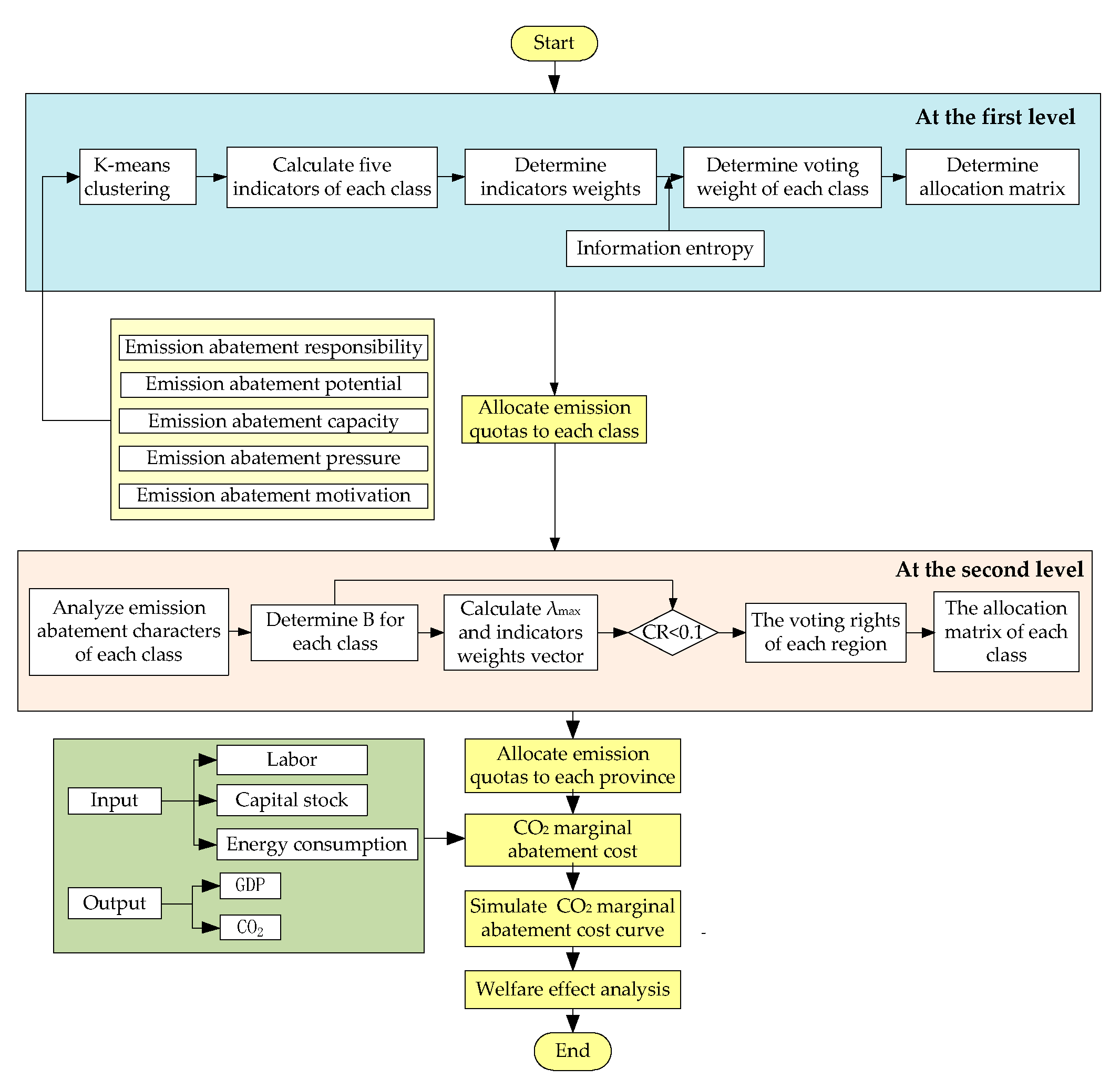
4.3. Allocation Results at the Second Level

Through the work of the above section, the national carbon quotas have been allocated to four classes. This section aims to allocate carbon quotas to each province within the same class. These provinces have the similar carbon emission characters. Thus, it is reasonable to explore their difference in carbon emission characteristics to allocate the emission quotas. Based on the analysis of the above section, the indicator weights within each class are defined, as follows.

The provinces that are included in class 1 have the strongest economic strength; emission reduction has the least influence on their economic development. Therefore, emissions abatement capacity should be paid the least attention in this class. Similarly, the urbanization levels and per capita disposable incomes of this class are also the highest. Besides, more attention should be paid to the demographics factor in the quota allocation of this class. Accordingly, the emission abatement pressure is considered to be the most important indicator. The technological innovation capabilities in this class of region are relatively high, so that they have more motivation to reduce carbon emissions, and emission abatement will not hurt their motivation. Therefore, this indicator does not require too much attention. On the whole, the relative importance of the five indicators is defined as: $x_4>x_2>x_1>x_5>x_3$.

The provinces that are contained in class 2 are innovative provinces, which have relatively strong technological innovation abilities. Accordingly, the emission abatement motivation is the least significant indicator. In the meantime, they are also well-developed provinces and have strong economic strengths. Thereby, the emission abatement capacity does not require too much attention. However, their strong economies generally depend on different models of economic development, and thereby a huge difference in the emission abatement responsibility exists. Along this line of thought, the emission abatement responsibility should be the primary concern in the quota allocation of this class. On the whole, the relative importance of the five indicators is defined as: $x_1>x_2>x_4>x_3>x_5$.

The provinces that are contained in class 3 are underdeveloped, so reducing the effect of emission abatement on the economic growth is necessary; the provinces with poorer economic strength should be assigned more carbon quota. Therefore, emission abatement capacity is the primary concern in this case. Additionally, there exists huge difference in emission abatement potential among the provinces of this class. Therefore, the emission abatement potential should be considered as the second key indicator in this case. The urbanization levels and per capita disposable incomes in this class of regions are relatively low. The corresponding abatement pressures are also low and they should be the least important. Based on this, the relative importance of the five indicators in this class is defined as: $x_3>x_2>x_1>x_5>x_4$.

The provinces that are included in class 4 are resource-based provinces, having large potential and space to mitigate carbon emissions. To encourage these provinces to apply more effective production ways and to develop modern industries, the emission abatement potential should be paid the most attention. Similar to class 3, the provinces of class 4 are underdeveloped provinces; to reduce the influence of emission mitigation on their economy, the emission abatement capacity should be the second key indicator to be considered. Besides, a huge difference in emission abatement responsibility exists, so this indicator also needs to be focused on. The relative importance of the five indicators in this class is defined as: $x_2>x_3>x_1>x_4=x_5$.

According to the above analysis, the indicators’ relative importance within a class are defined and presented in

Table 10. Pairwise comparison matrix of each class.

(a) Pairwise Comparison Matrix of Class 1
	$x_1$	$x_2$	$x_3$	$x_4$	$x_5$
$x_1$	1	1/3	5	1/5	3
$x_2$	3	1	7	1/3	5
$x_3$	1/5	1/7	1	1/9	1/3
$x_4$	5	3	9	1	7
$x_5$	1/3	1/7	3	1/7	1
(b) Pairwise Comparison Matrix of Class 2
	$x_1$	$x_2$	$x_3$	$x_4$	$x_5$
$x_1$	1	3	7	5	9
$x_2$	1/3	1	5	3	7
$x_3$	1/7	1/5	1	1/3	3
$x_4$	1/5	1/3	3	1	5
$x_5$	1/9	1/7	1/3	1/5	1
(c) Pairwise Comparison Matrix of Class 3
	$x_1$	$x_2$	$x_3$	$x_4$	$x_5$
$x_1$	1	1/3	1/5	5	3
$x_2$	3	1	1/3	7	5
$x_3$	5	3	1	9	7
$x_4$	1/5	1/7	1/9	1	1/3
$x_5$	1/3	1/5	1/7	3	1
(d) Pairwise Comparison Matrix of Class 4
	$x_1$	$x_2$	$x_3$	$x_4$	$x_5$
$x_1$	1	1/5	1/3	3	3
$x_2$	5	1	3	7	7
$x_3$	3	1/3	1	5	5
$x_4$	1/3	1/7	1/5	1	1
$x_5$	1/3	1/7	1/5	1	1

.

Table 11. The consistency test of each matrix.

The Pairwise Comparison Matrices	Matrix of Class 1	Matrix of Class 2	Matrix of Class 3	Matrix of Class 4
CR	0.0425	0.0530	0.0530	0.0304

illustrates the consistency test result of each matrix, which suggests that these matrices meet the consistency requirements. In the light of pairwise comparison matrix illustrated in Table 10, the indicators weights within a class can be derived and are shown in

Table 12. The weight of each indicator within classes in the light of the analytic hierarchy process (AHP).

Weight	Indicators
Classes	${\mathit{x}}_1$	${\mathit{x}}_2$	${\mathit{x}}_3$	${\mathit{x}}_4$	${\mathit{x}}_5$
Class 1	0.1289	0.2618	0.0336	0.5149	0.08
Class 2	0.5128	0.2615	0.0634	0.1290	0.0333
Class 3	0.1290	0.2615	0.5128	0.0333	0.0634
Class 4	0.1223	0.5140	0.2580	0.0529	0.0529

.

Table 13. The voting right of each province.

Classes	Provinces	Voting Rights
Class 1	Beijing	0.4150
	Tianjin	0.1022
	Shanghai	0.3037
	Jiangsu	0.0823
	Zhejiang	0.0968
Class 2	Liaoning	0.0917
	Anhui	0.1484
	Fujian	0.1629
	Shandong	0.0972
	Hubei	0.1496
	Hunan	0.1709
	Guangdong	0.1793
Class 3	Hebei	0.0519
	Jilin	0.0557
	Heilongjiang	0.0854
	Jiangxi	0.0744
	Henan	0.0613
	Guangxi	0.1017
	Hainan	0.0915
	Sichuan	0.0761
	Guizhou	0.0638
	Yunnan	0.1021
	Shaanxi	0.0452
	Gansu	0.1045
	Qinghai	0.0421
	Xinjiang	0.0442
Class 4	Shanxi	0.3408
	Inner Mongolia	0.4207
	Ningxia	0.2385

shows the voting right of each province.

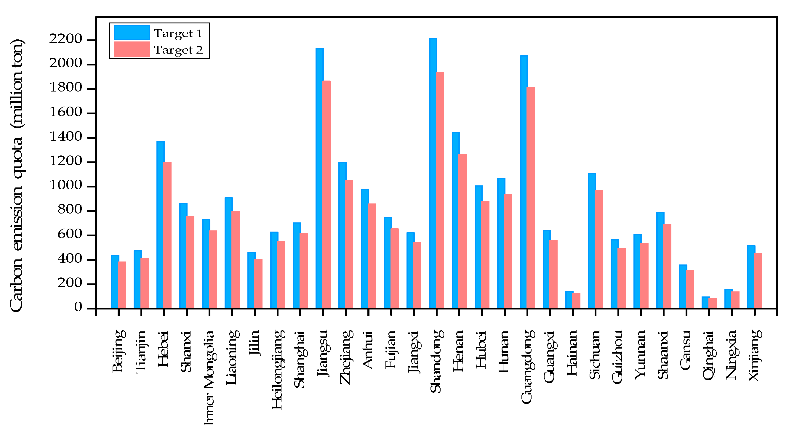
Based on the above analysis, the final carbon emission quotas of each province can be calculated and are listed in Figure 5. There are six provinces with carbon emission quotas exceeding 1000 Mt under target 1 and target 2, namely, Shandong, Jiangsu, Guangdong, Henan, Hebei, and Zhejiang. Among them, Shandong obtains the most carbon emission quota, with 2210.85 Mt and 1934.5 Mt under target 1 and 2, respectively. However, Ningxia, Hainan, and Qinghai get the least quotas, only accounting for less than 2%, among which Qinghai only obtains 95.3 Mt and 83.39 Mt under target 1 and 2, respectively.

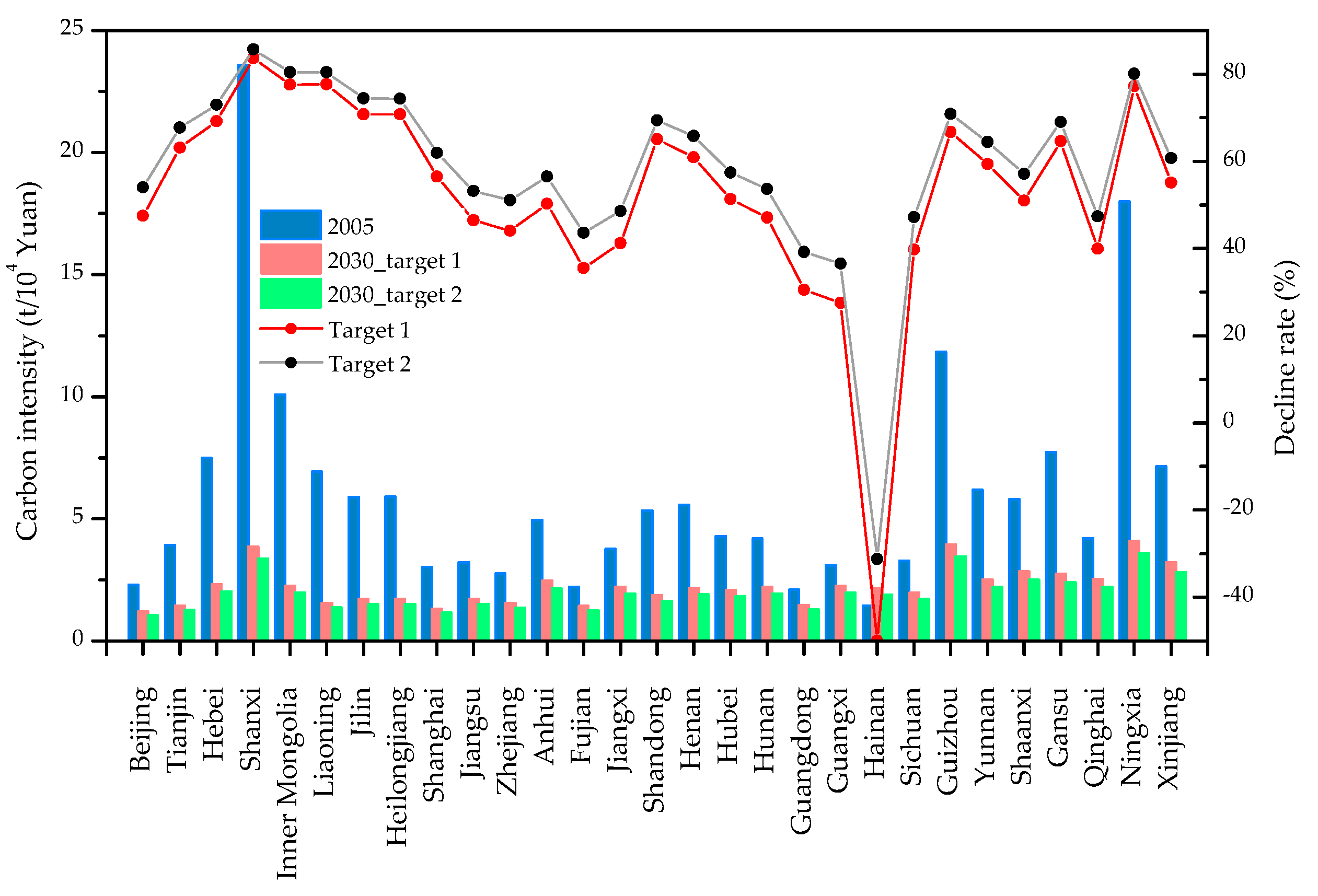
In the light of carbon emission quotas of all provinces, provincial carbon intensity in China in 2030 can be predicted. When comparing the carbon intensity of each province in 2030 with that in 2005, the decline rates of provincial carbon intensity during 2005–2030 are calculated. Figure 6 displays carbon intensity in 2005 and 2030 and corresponding decline rates of 29 provinces in China. The results suggest that the average carbon intensity in 2030 are, respectively, 1.93 t/10⁴ Yuan and 1.68 t/10⁴ Yuan under target 1 and target 2. Besides, the differences in terms of carbon intensity across regions in 2030 have narrowed when compared to 2005, which means that the proposed scheme can balance corresponding differences. According to the national target of 60–65%, all the provinces are grouped into four categories that are based on the decline rates under target 2, namely, Region A, Region B, Region C, and Region D.

Table 14. Provincial classification by carbon intensity.

Decline Rates	Regions	Provinces
<0	Region 1	Hainan
0–60%	Region 2	Beijing, Shanghai, Jiangsu, Zhejiang, Anhui, Fujian, Jiangxi, Hubei, Hunan, Guangdong, Guangxi, Sichuan, Shaanxi, Qinghai
60–70%	Region 3	Tianjin, Shandong, Henan, Yunnan, Gansu, Xinjiang
>70%	Region 4	Hebei, Shanxi, Inner Mongolia, Liaoning, Jilin, Heilongjiang, Guizhou, Ningxia

illustrates the classification result.

There is only one province in Region A, namely, Hainan, whose decreased rate of carbon intensity is negative. In other words, carbon intensity in 2030 is higher than that in 2005, which can reduce Hainan’s pressure in terms of emission reduction and enable Hainan to obtain benefits through selling excess quotas.

Region B contains 14 provinces, most of which are developed regions. Their decreasing amplitude of carbon intensity is below 60%, which suggests that the highly-efficient provinces undertake fewer burdens to reduce the emissions under the proposed model.

Region C includes Tianjin, Shandong, Henan, Yunnan, Gansu, and Xinjiang. Their emission reduction targets are close to national target, and emission mitigation obligations are between Region B and Region D. In other words, Region C bears the medium responsibility in terms of emissions abatement.

Region D includes eight provinces, e.g., Hebei and Shanxi, which are resource-based provinces. The decreasing amplitudes of provincial carbon intensity in this region are above 80%, and these provinces bear the greatest burden to reduce the carbon emissions. The statistical data illustrates that the carbon intensities of the eight provinces in 2005 are also the highest, whose average carbon intensity is 11.22 t/10⁴ Yuan. The economic developments of these provinces excessively rely on their own natural resources, thereby leading to higher carbon intensity. Accordingly, increasing the discharge standard of pollutants or eliminating the enterprises that fail to meet the standard may be an effective way of urging these regions to endeavor to mitigate their carbon emissions.

4.4. Welfare Effect Analysis of Final Allocation Results

All of the countries and regions should be treated equally in terms of the welfare effect obtained from the carbon trading market, which reflects the criterion of horizontal equity; the allocation method that can obtain the greatest welfare effect and make the regional differences in welfare effect the smallest and be accepted easily by these countries and regions. Hence, this section aims to discuss the performance of the proposed scheme from the perspective of a welfare effect. Three fundamental allocation schemes of initial quotas are studied for comparison. By simulating carbon trading market, welfare effect is measured using general market equilibrium. 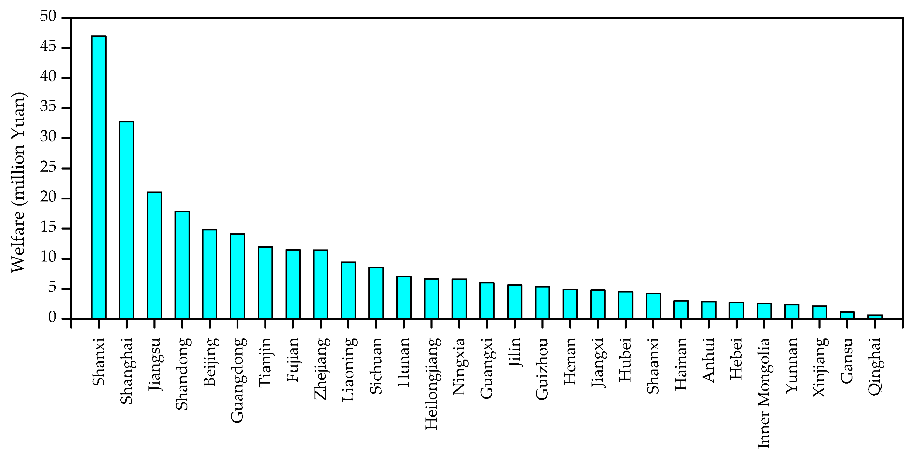Figure 7 depicts welfare effect of each province under targets 1. From Figure 7, it can be seen that Shanxi receives the most welfare through the carbon trading market, followed by Shanghai under target 1. As a resource-based province, Shanxi has been taking the development path of extensive production. Correspondingly, its marginal abatement cost is relatively low, that is, it does not need to pay too much for the reduction of same amount of CO₂ emissions. Thus, Shanxi can earn additional revenue by selling the carbon quota when the carbon trading market is launched. In addition, Shanghai is the most important economic, financial, and trading center in the whole country, whose value-added to the secondary industry only accounts for 29.83% and the economy is mainly driven by the tertiary industry. Based on this, its marginal abatement cost is relatively high and needs to pay a lot for completing emission reduction target by itself. Under these circumstances, Shanghai can purchase quota from carbon trading market at a relatively lower price than the marginal abatement cost. Along this line of thought, it can obtain additional welfare when compared to the situation without carbon trading. 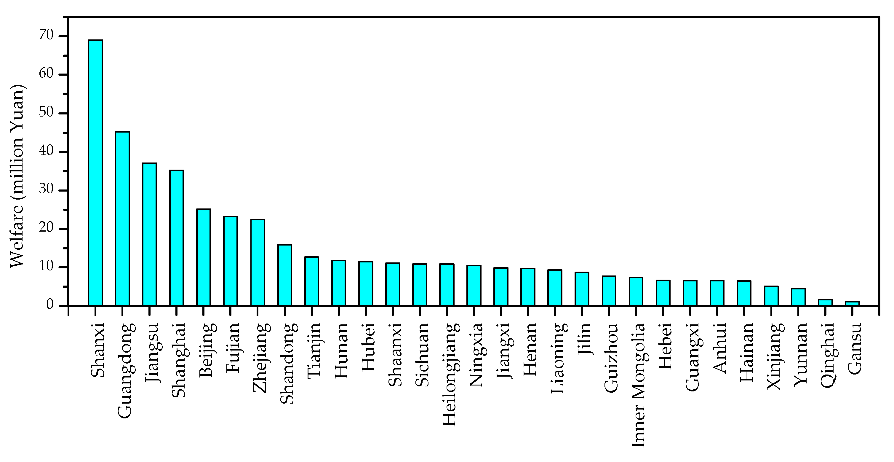Figure 8 depicts the welfare effect of each province under targets 2. Similar to the situation of target 1, Shanxi still obtains the most welfare and Guangdong takes the second place, while Gansu obtains the least welfare in this carbon trading. We can see that the proposed model can balance the welfare effect across provinces with different carbon emission characteristics. However, the welfare effect under the allocation scheme that is based on a single indicator will have a certain tendency in the light of carbon emission characteristic. For example, the quota allocation scheme in terms of historical emissions will result in more welfare for province with more CO₂ emissions, which is unfair to other provinces using resources effectively and is not conducive to energy saving and emission reduction. If the quotas are allocated according to GDP, the provinces having powerful economic strengths will obtain more welfare from the carbon trading market. However, it will impose an excessive burden on the underdeveloped provinces, which is not conducive to their economic development, thereby leading to an increasing gap between the rich and the poor. A population-based allocation scheme will benefit the province with more population, which neglects the needs of economic development. Therefore, no matter what type of indicator is employed in allocation, the tendency of the welfare effect always exists. On this basis, these three fundamental schemes based on a single indicator are difficult to satisfy all provinces. Thus, this paper proposes a bi-level weighted voting model, comprehensively taking various indicators into consideration. In this model, every province can be taken care of through voting for their preferred scheme, instead of focusing on the prominent province in terms of a single indictor, as in the single indicator allocation scheme. Next, we continue to explore the superiority of this proposed model.

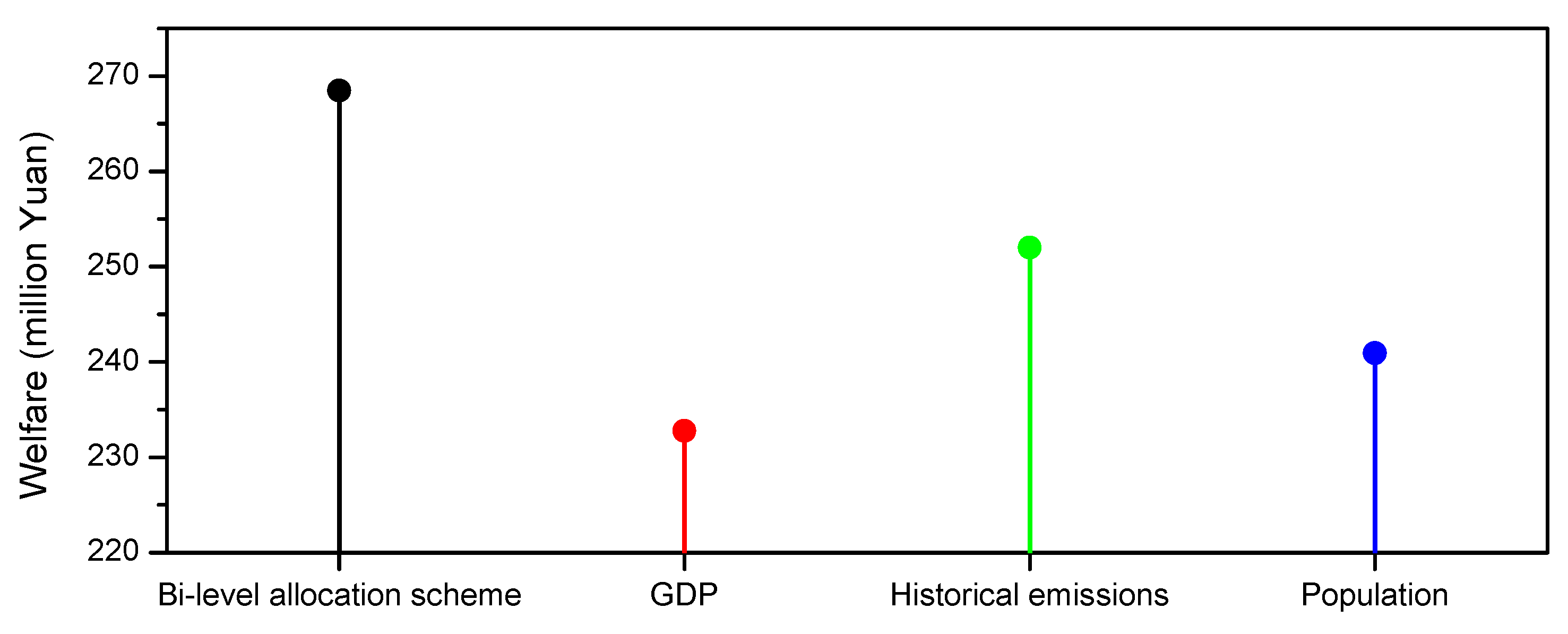
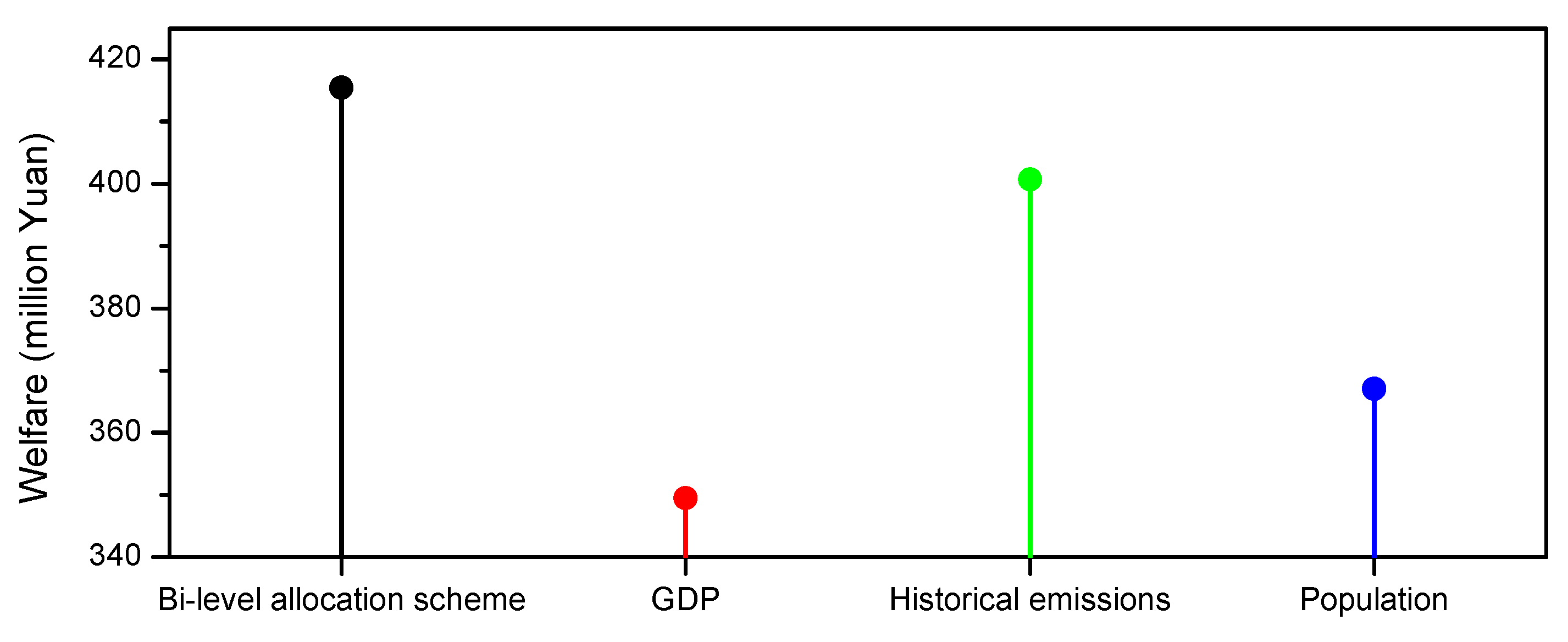
Three fundamental allocation schemes are studied for comparison to verify the performance of this proposed model. First, we study the welfare effects under different allocation schemes from the perspective of the total amount. Figure 9 and Figure 10, respectively, depict the total welfare of different quota allocation schemes under target 1 and target 2. From them, it can be seen that this model produces the greatest welfare effect, both under the target 1 and the target 2, followed by the allocation scheme that is based on historical emissions, while the GDP-based allocation scheme produces the least.

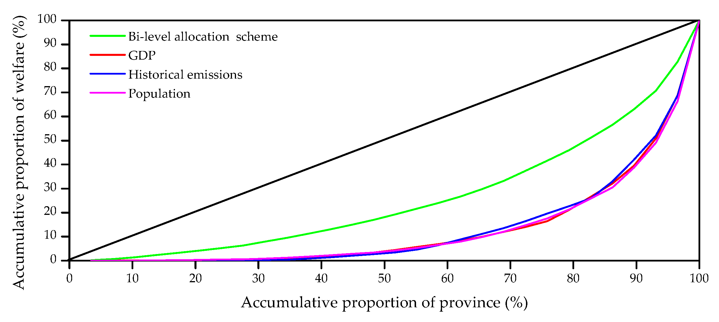
Subsequently, we study the welfare effect distribution across provinces under different allocation schemes. The Lorentz curve is proposed in order to study the distribution of national incomes among persons. This paper employs the Lorentz curve to measure the welfare distribution across the provinces. Figure 11 demonstrates the Lorentz curves of the proposed scheme, GDP-based scheme, historical emissions-based scheme, and population-based scheme under target 1, as well as the curve of absolute equity for comparison. From Figure 11, it can be seen that the Lorentz curve of the proposed allocation scheme is closer to the curve of absolute equity when compared to the other three schemes. 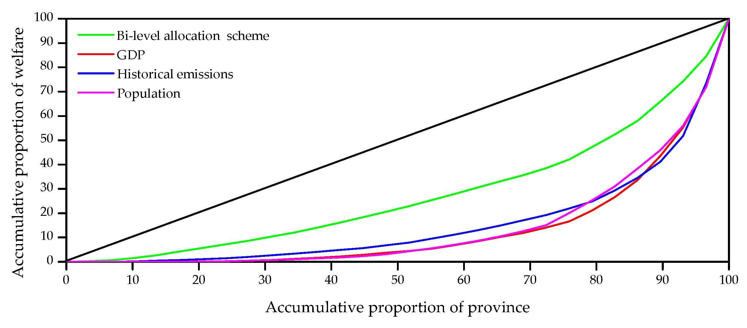Figure 12 depicts the Lorentz curves of four allocation schemes under target 2 and the curve of absolute equity. Similar to Figure 11, the Lorentz curve of the proposed scheme is the closest to the absolute equity curve. Based on the above analysis, it can be seen that the welfare effect of the whole country is the greatest, and the differences in terms of the welfare effect across provinces are the smallest when the bi-level allocation scheme is adopted. Therefore, the proposed allocation scheme can not only encourage all provinces to effectively reduce carbon emission intensity, but also be easily accepted by all provinces.

5. Conclusions and Policy Implications

This paper proposed a novel model, called bi-level allocation based on weighted voting method. This allocation model divides an allocation process into two levels and employs different allocation approaches for different levels. Through the above analysis, the main conclusions and policy implications can be drawn.

(1)

In the light of carbon emission characteristics, the k-means clustering method clusters 29 China’s provinces into four categories, which contain: (a) five richest municipalities and provinces, namely, Beijing, Tianjin, Shanghai, Jiangsu, and Zhejiang; (b) the developed and innovative provinces with high per capita GDP, per capita disposal incomes, and strong technical innovation ability, such as Shandong and Guangdong; (c) the underdeveloped provinces, mainly distributed in the central and western China, e.g., Gansu and Guizhou; and, (d) the resource-based provinces characterized by high proportion of heavy industry and high carbon intensity, containing Shanxi, Inner Mongolia, and Ningxia.

(2)

The allocation schemes that are based on historical emissions, GDP and population are considered as three fundamental schemes to assign carbon emission quota and different regions have different preferences for allocation schemes. This paper employs the weighted voting model to allocate carbon quota at each level to balance the preferences of each region. At the first level, information entropy theory is utilized to determine the indicator weights. The result suggests that emission abatement responsibility is the most significant for quota allocation, followed by emission abatement capacity, while emission abatement pressure is the least important. At the second level, AHP is employed to determine the indicator weights within a class. In reality, the specific pairwise comparison matrix can be adjusted according to relevant policies, which increase the flexibility of the proposed scheme.

(3)

The emission abatement responsibilities are borne by all provinces of China, but the responsibility shares are various, which are related to their respective carbon emission characteristics. According to national target of 60–65%, all of the provinces are grouped into four categories based on the decline rates under target 2, namely, Region A, Region B, Region C, and Region D, and the emission reduction burden is gradually increased from Region A to Region D. The empirical results illustrate that the differences in carbon intensity across regions have narrowed in 2030 when compared to 2005, which means that the proposed scheme can balance the differences in carbon intensity among regions.

(4)

In order to verify the rationality of the proposed scheme, the national carbon trading market is simulated and the welfare effect for each province is measured. Simulation results show the proposed model can balance the welfare effect across provinces with different carbon emission characteristics. Specifically, we explore the superiority of this proposed model in terms of the welfare effect. Here, the Lorentz curve is employed to measure the welfare distribution across provinces. The results indicate that the welfare effect of the whole country is the largest, and the differences in welfare effect across provinces are the smallest when the bi-level allocation scheme is adopted. Therefore, the proposed allocation scheme can not only encourage all provinces to reduce carbon emission intensity effectively, but it can also be easily accepted by all provinces.

Our empirical results have several important implications. Firstly, the welfare effect is measured using the market general equilibrium model by simulating the carbon trading market. Results indicate all 29 provinces will receive welfares from the carbon trading market relative to the case without carbon trading market. However, until now only the power generation sector is included in the national carbon trading scheme, which leads to a lack of liquidity for carbon quota, and it thereby affects the welfare of each province obtained from the carbon trading market. More regions and sectors included in this scheme can promote the emission quotas to flow fully in the market and form a more instructive equilibrium price for carbon quota. The government should use the power generation industry as a breakthrough to gradually expand the scope of the industry and region involved in the carbon market. Along this line of thought, the market efficiency and the welfare effect will be undoubtedly improved. Secondly, the initial quota allocation mechanism has great impact on the welfare effect of each province obtained from the carbon trading market. Additionally, the reasonable carbon quota allocation is not only the guarantee for completing abatement obligations, but is also the basis for China to launch a national carbon trading market. The government should fully understand the actual situation of each region, while taking into account a series of factors, such as economic level, population size, historical emissions, and scale effect when formulating emission reduction targets. Thirdly, China′s previous economic development model was extensive, which has brought severe environmental problems. It is predictable that, with the price of carbon emission increasing, regions will have no choice to apply cleaner energy or more effective production ways. Accordingly, with the reduction of carbon emissions, China will inevitably experience a deep revolution in the structures of economy and energy consumption.

Although this paper can offer several effective advices for decision-maker in designing environmental policies, there are still some issues to be solved. Quota allocation is a complex issue and many factors need to be considered. In future research, more factors affecting the implementation of emission abatement policies should be considered to construct a more comprehensive quota allocation scheme. In addition, the regional cooperation is believed to be in favor of carbon emissions abatement. Although we have studied the regional quota allocation, we do not take the collaborative impact of carbon emission abatement across provinces into account, which may generate false analysis [56]. Therefore, introducing the cooperative game theory can expand further researches.

References

1. Lee, S.; Chong, W.O. Causal relationships of energy consumption, price, and CO2 emissions in the US building sector. Resour. Conserv. Recycl. 2016, 107, 220–226. [Google Scholar] [CrossRef]
2. Cai, W.; Lai, K.; Liu, C.H.; Wei, F.F.; Ma, M.; Jia, S.; Jiang, Z.G.; Lv, L. Promoting sustainability of manufacturing industry through the lean energy-saving and emission-reduction strategy. Sci. Total Environ. 2019, 665, 23–32. [Google Scholar] [CrossRef] [PubMed]
3. Dong, F.; Yu, B.L.; Hadachin, T.; Dai, Y.J.; Wang, Y.; Zhang, S.N. Drivers of carbon emission intensity change in China. Resour. Conserv. Recycl. 2018, 129, 187–201. [Google Scholar] [CrossRef]
4. Guo, R.; Zhao, Y.R.; Shi, Y.; Li, F.T.; Hu, J.; Yang, H.Z. Low carbon development and local sustainability balance perspective from a carbon. Resour. Conserv. Recycl. 2017, 122, 270–279. [Google Scholar] [CrossRef]
5. Tian, X.; Dai, H.C.; Geng, Y.; Huang, Z.; Masui, T.H.; Fujita, T. The effects of carbon reduction on sectoral competitiveness in China: A case of Shanghai. Appl. Energy 2017, 197, 270–278. [Google Scholar] [CrossRef]
6. Bi, C.; Jia, M.N.; Zeng, J.J. Nonlinear effect of public infrastructure on energy intensity in China: A panel smooth transition regression approach. Sustainability 2019, 11, 629. [Google Scholar] [CrossRef]
7. Xian, Y.J.; Wang, K.; Wei, Y.M.; Huang, Z.M. Would China’s power industry benefit from nationwide carbon emission permit trading? An optimization model-based ex post analysis on abatement cost savings. Appl. Energy 2019, 235, 978–986. [Google Scholar] [CrossRef]
8. Zhou, P.; Zhang, L.; Zhou, D.Q.; Xia, W.J. Modeling economic performance of interprovincial CO2 emission reduction quota trading in China. Appl. Energy 2013, 112, 1518–1528. [Google Scholar] [CrossRef]
9. Han, R.; Tang, B.J.; Fan, J.L.; Liu, L.C.; Wei, Y.M. Integrated weighting approach to carbon emission quotas: An application case of Beijing-Tianjin-Hebei region. J. Clean. Prod. 2016, 131, 448–459. [Google Scholar] [CrossRef]
10. Shuai, C.Y.; Shen, L.; Jiao, L.; Wu, Y.; Tan, Y. Identifying key impact factors on carbon emission: Evidences from panel and time-series data of 125 countries from 1990 to 2011. Appl. Energy 2017, 187, 310–325. [Google Scholar] [CrossRef]
11. Pang, R.Z.; Deng, Z.Q.; Chiu, Y.H. Pareto improvement through a reallocation of carbon emission quotas. Renew. Sustain. Energy Rev. 2015, 50, 419–430. [Google Scholar] [CrossRef]
12. Chiu, Y.H.; Lin, J.C.; Su, W.N.; Liu, J.K. An efficiency evaluation of the EU’s allocation of carbon emission allowances. Energy Sources Part B Econ. Plan. Policy 2015, 10, 192–200. [Google Scholar] [CrossRef]
13. Pan, X.Z.; Teng, F.; Wang, G.H. Sharing emission space at an equitable basis: Allocation scheme based on the equal cumulative emission per capita principle. Appl. Energy 2014, 113, 1810–1818. [Google Scholar] [CrossRef]
14. Pan, X.Z.; Teng, F.; Wang, G.H. A comparison of carbon allocation schemes: On the equity-efficiency tradeoff. Energy 2014, 74, 222–229. [Google Scholar] [CrossRef]
15. Pan, X.Z.; Teng, F.; Ha, Y.; Wang, G.H. Equitable access to sustainable development: Based on the comparative study of carbon emission rights allocation schemes. Appl. Energy 2014, 130, 632–640. [Google Scholar] [CrossRef]
16. Ciscar, J.C.; Ciscar, J.C.; Saveyn, B.; Soria, A.; Szabo, L.; Van Regemorter, D.; Van Ierland, T. A comparability analysis of global burden sharing GHG reduction scenarios. Energy Policy 2013, 55, 73–81. [Google Scholar] [CrossRef] [Green Version]
17. Sanin, M.E.; Violante, F.; Mansanet-Bataller, M. Understanding volatility dynamics in the EU-ETS market. Energy Policy 2015, 82, 321–331. [Google Scholar] [CrossRef] [Green Version]
18. Li, W.; Jia, Z. The impact of emission trading scheme and the ratio of free quota: A dynamic recursive CGE model in China. Appl. Energy 2016, 174, 1–14. [Google Scholar] [CrossRef]
19. Huang, H.; Roland-Holst, D.; Springer, C.; Lin, J.; Cai, W.; Wang, C. Emissions trading systems and social equity: A CGE assessment for China. Appl. Energy 2019, 235, 1254–1265. [Google Scholar] [CrossRef]
20. Zetterberg, L.; Wråke, M.; Sterner, T.; Fischer, C.; Burtraw, D. Short-run allocation of emissions allowances and long-term goals for climate policy. Ambio 2012, 41, 23–32. [Google Scholar] [CrossRef]
21. Zhou, X.; James, G.; Liebman, A.; Dong, Z.Y.; Ziser, C. Partial carbon permits allocation of potential emission trading scheme in Australian electricity market. IEEE Trans. Power Syst. 2009, 25, 543–553. [Google Scholar] [CrossRef]
22. Hong, T.; Koo, C.; Lee, S. Benchmarks as a tool for free allocation through comparison with similar projects: Focused on multi-family housing complex. Appl. Energy 2014, 114, 663–675. [Google Scholar] [CrossRef]
23. Edwards, T.H.; Hutton, J.P. Allocation of carbon permits within a country: A general equilibrium analysis of the United Kingdom. Energy Econ. 2001, 23, 371–386. [Google Scholar] [CrossRef]
24. Wiśnicki, B.; Chybowski, L.; Czarnecki, M. Analysis of the efficiency of port container terminals with the use of the data envelopment analysis method of relative productivity evaluation. Manag. Syst. Prod. Eng. 2017, 25, 9–15. [Google Scholar] [CrossRef]
25. Wang, S.; Chu, C.; Chen, G.; Peng, Z.; Li, F. Efficiency and reduction cost of carbon emissions in China: A non-radial directional distance function method. J. Clean. Prod. 2016, 113, 624–634. [Google Scholar] [CrossRef]
26. Zhang, Y.J.; Hao, J.F. Carbon emission quota allocation among China’s industrial sectors based on the equity and efficiency principles. Ann. Oper. Res. 2017, 255, 117–140. [Google Scholar] [CrossRef]
27. Feng, C.P.; Chu, F.; Ding, J.J.; Bi, G.B.; Liang, L. Carbon Emissions Abatement (CEA) allocation and compensation schemes based on DEA. Omega 2015, 53, 78–89. [Google Scholar] [CrossRef]
28. Ji, X.; Li, G.; Wang, Z.H. Allocation of emission permits for China’s power plants: A systemic Pareto optimal method. Appl. Energy 2017, 204, 607–619. [Google Scholar] [CrossRef]
29. An, Q.X.; Wen, Y.; Xiong, B.B.; Yang, M.; Chen, X.H. Allocation of carbon dioxide emission permits with the minimum cost for Chinese provinces in big data environment. J. Clean. Prod. 2017, 142, 886–893. [Google Scholar] [CrossRef]
30. Kong, Y.; Dong, S. A carbon-intensity based carbon allowance allocation scheme among enterprises in shenzhen. Econ. Econ. 2016, 1, 2–17. [Google Scholar]
31. Wang, T.; Wang, X.; Gong, Y.; Jiang, C.; Xiong, F.; Li, L. Initial allocation of carbon emission permits in power systems. J. Mod. Power Syst. Clean Energy 2017, 5, 239–247. [Google Scholar] [CrossRef]
32. Yu, S.; Wei, Y.M.; Wang, K. Provincial allocation of carbon emission reduction targets in china: An approach based on improved fuzzy cluster and Shapley value decomposition. Energy Policy 2014, 66, 630–644. [Google Scholar] [CrossRef]
33. Yu, S.; Wei, Y.M.; Fan, J.; Zhang, X.; Wang, K. Exploring the regional characteristics of inter-provincial CO2 emissions in China: An improved fuzzy clustering analysis based on particle swarm optimization. Appl. Energy 2012, 92, 552–562. [Google Scholar] [CrossRef]
34. Yang, M.; An, Q.; Ding, T.; Yin, P.; Liang, L. Carbon emission allocation in china based on gradually efficiency improvement and emission reduction planning principle. Ann. Oper. Res. 2017, 1, 1–17. [Google Scholar] [CrossRef]
35. Qin, Q.; Liu, Y.; Li, X.; Li, H. A multi-criteria decision analysis model for carbon emission quota allocation in China’s east coastal areas: Efficiency and equity. J. Clean. Prod. 2017, 168, 410–419. [Google Scholar] [CrossRef]
36. Zhang, Y.J.; Wang, A.D.; Da, Y.B. Regional allocation of carbon emission quotas in china: Evidence from the Shapley value method. Energy Policy 2014, 74, 454–464. [Google Scholar] [CrossRef]
37. Voigt, S.; De Cian, E.; Schymura, M.; Verdolini, E. Energy intensity developments in 40 major economies: Structural change or technology improvement? Energy Econ. 2014, 41, 47–62. [Google Scholar] [CrossRef] [Green Version]
38. Sequeira, T.; Santos, M. Education and energy intensity: Simple economic modelling and preliminary empirical results. Sustainability 2018, 10, 2625. [Google Scholar] [CrossRef]
39. Li, H.; Lo, K.; Wang, M.; Zhang, P.; Xue, L. Industrial energy consumption in Northeast China under the revitalisation strategy: A decomposition and policy analysis. Energies 2016, 9, 549. [Google Scholar] [CrossRef]
40. Song, Y.; Zhang, M.; Zhou, M. Study on the decoupling relationship between CO2 emissions and economic development based on two-dimensional decoupling theory: A case between China and the United States. Ecol. Indic. 2019, 102, 230–236. [Google Scholar] [CrossRef]
41. Hao, Y.; Peng, H.; Temulun, T.; Liu, L.Q.; Mao, J.; Lu, Z.N. How harmful is air pollution to economic development? New evidence from PM2.5 concentrations of Chinese cities. J. Clean. Prod. 2018, 172, 743–757. [Google Scholar] [CrossRef]
42. Dhakal, S. Urban energy use and carbon emissions from cities in China and policy implications. Energy Policy 2009, 37, 4208–4242. [Google Scholar] [CrossRef]
43. Zhang, Y.J.; Da, Y.B. Decomposing the changes of energy-related carbon emissions in China: Evidence from the PDA approach. Nat. Hazards 2013, 69, 1109–1122. [Google Scholar] [CrossRef]
44. Piao, M.; Piao, Y.; Lee, J.Y. Symmetrical uncertainty-based feature subset generation and ensemble learning for electricity customer classification. Symmetry 2019, 11, 498. [Google Scholar] [CrossRef]
45. Chybowski, L.; Twardochleb, M.; Wiśnicki, B. Multi-criteria decision making in components importance analysis applied to a complex marine system. Naše More Znan. Stručni Časopis More I Pomor. 2016, 63, 264–270. [Google Scholar]
46. Chybowski, L.; Gawdzińska, K. On the present state-of-the-art of a component importance analysis for complex technical systems. New Adv. Inf. Syst. Technol. 2016, 445, 691–700. [Google Scholar]
47. Chybowski, L.; Gawdzińska, K. On the possibilities of applying the AHP method to a multi-criteria component importance analysis of complex technical objects. New Adv. Inf. Syst. Technol. 2016, 445, 701–710. [Google Scholar]
48. Shang, Y.L. Unveiling robustness and heterogeneity through percolation triggered by random-link breakdown. Phys. Rev. E 2014, 90, 032820. [Google Scholar] [CrossRef]
49. Shang, Y.L. Impact of self-healing capability on network robustness. Phys. Rev. E 2015, 91, 042804. [Google Scholar] [CrossRef]
50. Shannon, C.E. A mathematical theory of communication. Bell Syst. Tech. J. 1948, 27, 379–423. [Google Scholar] [CrossRef]
51. Chen, S.Y. Shadow price of industrial carbon dioxide: Parametric and non-Parametric method. World Econ. 2010, 33, 93–111. [Google Scholar]
52. Tu, Z.G. The shadow price of industrial SO2 emission: A new analytic framework. China Econ. Q. 2009, 9, 259–282. [Google Scholar]
53. Nordhaus, W.D. The cost of slowing climate change: A survey. Energy J. 1991, 12, 37–65. [Google Scholar] [CrossRef]
54. Shan, H. Reestimating the capital stock of China: 1952~2006. J. Quant. Tech. Econ. 2008, 25, 17–31. [Google Scholar]
55. Chen, J.D.; Cheng, S.L.; Son, M.L.; Wu, Y.Y. A carbon emissions reduction index: Integrating the volume and allocation of regional emissions. Appl. Energy 2016, 184, 1154–1164. [Google Scholar] [CrossRef]
56. Shang, Y.L. Resilient multiscale coordination control against adversarial nodes. Energies 2018, 11, 1844. [Google Scholar] [CrossRef]
Figure 1. Research framework.
Energies 12 02118 g001
Figure 2. Marginal abatement cost curve.
Energies 12 02118 g002
Figure 3. The clustering results based on carbon emission characteristics.
Energies 12 02118 g003
Figure 4. The carbon emission characteristics of four classes.
Energies 12 02118 g004
Figure 5. The carbon emission quotas of each region.
Energies 12 02118 g005
Figure 6. Carbon intensity and decline rates of 29 provinces in China.
Energies 12 02118 g006
Figure 7. Welfare effect of each province in descending order under target 1.
Energies 12 02118 g007
Figure 8. Welfare effect of each province in descending order under target 2.
Energies 12 02118 g008
Figure 9. Total welfares of different quota allocation schemes under target 1.
Energies 12 02118 g009
Figure 10. Total welfares of different quota allocation schemes under target 2.
Energies 12 02118 g010
Figure 11. The Lorentz curve of welfare effect under target 1.
Energies 12 02118 g011
Figure 12. The Lorentz curve of welfare effect under target 2.
Energies 12 02118 g012