Article

Analyzing the Performance and Control of a Hydronic Pavement System in a District Heating Network

1
Division of Energy Systems, Department of Management and Engineering, Linköping University, SE-581 83 Linköping, Sweden
2
Division of Building, Energy and Environment Technology, Department of Technology and Environment, University of Gävle, SE-801 76 Gävle, Sweden
*
Author to whom correspondence should be addressed.
Louise Ödlund (former Trygg).
Energies 2019, 12(11), 2078; https://doi.org/10.3390/en12112078
Submission received: 29 April 2019 / Revised: 27 May 2019 / Accepted: 27 May 2019 / Published: 30 May 2019
(This article belongs to the Special Issue District Heating and Cooling Networks)

Abstract

:
A hydronic pavement system (HPS) is an alternative method to clear snow and ice, which avoids the use of salt, sand, and fossil fuel in conventional snow clearance, and minimizes the risk of accidents. The aim is to analyze the performance of different control strategies for a 35,000 m2 HPS utilizing heat from a district heating and cooling (DHC) system. The key performance indicators are (1) energy performance of the HPS, and (2) primary energy use, (3) electricity production and (4) greenhouse gas (GHG) emissions from the DHC system. The methodology uses a simulation model of the HPS and an optimization model of the DHC system. Three operational strategies are analyzed: A reference scenario based on the current control strategy, and scenarios where the HPS is shut down at temperatures below −10 °C and −5 °C. The study shows that the DHC return temperature is suitable for use. By operational strategies, use during peak demand in the DHC system can be avoided, resulting in reduced use of fossil fuel. Moreover, the energy use of the HPS could be reduced by 10% and the local GHG emissions by 25%. The study emphasizes that the HPS may have positive effects on global GHG emissions, as it enables electricity production from renewable resources.

1. Introduction

In 1976, Sweden established the following definition for the heating of ground surfaces such as pavement areas: “Ground heat refers to devices for raising the surface temperature in order to avoid slipping, keeping the surface free of snow and ice or prolonging the vegetation period” [1]. Moreover, a system of 2000 m2 was installed in downtown Klamath Falls (Oregon, USA) in 1948 [2]. It operated for 50 years before being replaced due to external corrosion of the iron pipes [3]. The systems of today make use of electrical, infrared or, most commonly, hydronic techniques [4,5]. A hydronic pavement system (HPS) is a technique in which heat is transported in pipes embedded in the pavement structure using circulating water or other liquid heat media.
HPS can utilize different energy sources, such as geothermal energy, district heating or solar, and in some cases, it is also combined with thermal storage [6]. A review conducted by Lund and Boyd [7] states that an area of 2,500,000 m2 world-wide is heated by HPS utilizing geothermal energy, with required power of 130–180 W/m2 [7]. In addition, standalone solutions can be found, particularly in airports [8,9,10,11,12], and bridge decks [13,14]. In Sweden, there are 400 systems utilizing district heating as a heat source with annual use of 150–200 GWh [15]. The technique is increasingly common in for example Iceland, as Gunnlaugsson et al. [16] mention that systems such as HPS may utilize the low-grade heat of district heating return water.
Pan et al. [6] state that the technology of HPS is not only suitable for melting snow and ice. Pavements are exposed to a large amount of solar radiation, causing the pavement to reach temperatures of 55–75 °C [17]. This can impair the performance of the material, as well as causing urban heat islands [6,18]. A possible solution is to use pavements for energy harvesting [19], with pipes embedded in the structure channeling away the heat for immediate use elsewhere or for seasonal energy storage, to be used by a DHC system, for electrical purposes or recharging [6].
When compared to conventional snow clearance, the most common arguments in favor of using an HPS are the avoidance of sand, of potential material damage from conventional snow clearance, and of salt with its negative local environmental effects [20,21,22,23,24,25,26]. Moreover, conventional snow clearance contributes to greater greenhouse gas (GHG) emissions than HPS [11,27], since HPS enables the use of renewable energy, compared with the use of fossil fuel to operate heavy machinery as snow plows. Furthermore, it is desirable to avoid heavy machinery in crowded areas, which also reduces the risk of material damage to the pavement structure or its surroundings [1,28,29]. Crowded areas, such as commercial streets, squares, entrances, stairs or other areas with intensive use, are suitable areas for HPS [1]. Figure 1 displays such areas, a square and walkway, in the central parts of Linköping, Sweden, which is the location of this study.
The most common cause of accidents involving pedestrians, often older people, in Sweden is slipping, with 74% caused by snow and ice formation [30]. The accidents tend to occur in central areas [31,32] that are suitable for HPS. A study conducted in Sweden by Carlsson et al. [31] indicates that 80% of slipping accidents could be prevented by HPS. Moreover, studies indicate that the cost of injured pedestrians is more than four times higher than the winter maintenance. Accordingly, it has been shown to be cost-efficient to invest more in winter maintenance in pedestrian areas from a national perspective [32,33]. A study made by Nevalainen Henaes [27] in 2018 in Lund, Sweden, put the estimated construction cost of an HPS at 100 EUR/m2, whilst the maintenance cost is the same as conventional snow removal at 3 EUR/m2. The case study concludes the annual cost of slipping accidents to be 90 EUR/m2.
A control strategy for the HPS may be used in order to balance performance criteria, environmental criteria, and energy use [34]. Other studies have proposed ideas to minimize energy use, e.g., by stop heating during cold sub-zero temperatures and, thus, reduce the energy use [34,35]. Moreover, there is extensive research done to study strategies by steady-state models, as well as transient models, assessing energy use for different specific weather phenomena and locations [34,35,36], and many studies have been done in connection to geothermal heating [5]. However, this research intends to study a control strategy on an HPS utilizing district heating during a whole heating season using a transient model.
The national targets of Sweden, originating from the targets of the European Council [37], state that by 2020 GHG emissions shall be decreased by 40% (relative to 1990) and no net emissions shall occur by 2045. By 2020, the share of renewable energy shall be 50% of total energy use, and by 2040 electricity production shall be from 100% renewable resources [38,39]. The Swedish government [38] also stated in 2008 that fossil fuel is not to be used for heating purposes. This has led energy companies operating DHC system to phase out fossil fuel from their production by 2030 or by 2025, as some companies have committed to [40]. District heating utilizing the technology of combined heat and power (CHP) plants is said to provide an opportunity to make use of energy that would otherwise be wasted [38,39].
Studies emphasize the role of the CHP technique in the energy transition from fossil fuel to renewable resources [41,42,43,44]. Furthermore, considering the work of reducing GHG emissions, the potential electricity output from European CHP plants could be more than doubled [45]. On a global level, there is a low utilization and low awareness of the benefits of DHC and there is a potential for DHC systems to be a viable option of the future energy system [46]. However, studies also point to the unclear role of a DHC system in a future energy system, where questions regarding surplus electricity from intermittent sources and future access to conventional fuel as waste and biofuel are unexplored [47]. Stankeviciute et al. [45] argue that competition regarding biomass between the transport sector and other sectors will act as a limitation on the potential of CHP. The potential for a reduction in global GHG emissions highly depends on whether biofuel is seen as a limited or unlimited resource and on the alternative use of biofuel [48]. Studies also highlight potential issues where CHP plants are unprofitable in the future Nordic market, with a prevailing trend of heat-only boilers replacing CHP plants in DHC production [49].
Achieving low return temperatures is an important factor in obtaining an efficient DHC system, as it may increase the heat recovery from flue gas condensation and electricity generation in the CHP plants, as well as increasing the potential use of excess heat from industrial processes [50,51]. Moreover, the economic value of a reduced return temperature varies between 0.05 and 0.5 EUR/MWh, °C [52]. The average return temperature in Swedish DHC systems is 47.2 °C [50]. In order to have an efficient system, it is necessary to have as large difference as possible in the supply and return temperature [50], and in a future fourth generation of DHC systems, the supply temperature will most likely be reduced [53]. It will, therefore, be even more important to achieve low return temperatures, and in this work, an HPS utilizing the return temperatures of the DHC system can make a useful contribution.
The aim of this paper is to analyze the consequences of different control strategies for an HPS in a DHC network. The key performance indicators are (1) energy performance of the HPS, (2) the resulting primary energy use, (3) electricity production and (4) greenhouse gas emissions from the DHC system. The study was conducted by using a unique transient model and simulating three scenarios for operations of the HPS. Thereafter, the results were analyzed in the DHC system settings using an optimization model.
The main contribution of this work is the study of the environmental effects of an HPS, in terms of local GHG emissions and the effects on a global level. Also, as a contribution, the unique simulation model created in ANSYS software utilizing weather data of outdoor temperature, precipitation, wind, and solar irradiance enables detailed studies on how operational strategies may contribute to more efficient energy use.

2. Method

A framework including the development of a numerical simulation model and an optimization model was designed for this study, presented in Figure 2. A transient simulation model of the HPS system was created using the software ANSYS® Workbench™ and the patch ANSYS® CFX® Release 18.0 [54]. Three scenarios are analyzed in this setup. Data collection of material and weather properties plus boundary equations are inputs to the transient simulation model of the HPS. The simulation results are then scaled up to a larger system area, and the time step is converted into a flexible time division suitable for larger energy systems by using the software Converter [55]. The scenarios are then analyzed within the scope of the DHC system using the linear optimization program MODEST [56]. Section 2.1 and Section 2.2 present the software tools used in the study, while Section 3 and Section 4 describes the design of the scenario study as well as design and use of the software tools.

2.1. The Simulation Software ANSYS

The ANSYS software is an engineering simulation platform used to analyze how product designs will behave in an operative environment. The tool ANSYS CFX used in this study is general purpose computational fluid dynamics software capable of modeling, e.g., transient flows, heat transfer, and thermal radiation. The governing equations in ANSYS CFX are the unsteady Navier–Stokes equations [57] in their conservation form, which describe momentum, heat, and mass transfer. ANSYS uses the finite element method to reach a numerical solution, by iteratively solving the equations for each element and in so doing deriving a full picture of the flow in the model [58].

2.2. The Optimization Software MODEST

MODEST, short for “model for optimization of dynamic energy systems with time-dependent components and boundary conditions”, is a optimization software utilizing linear programming which was developed at Linköping University [59]. MODEST is structured according to energy flows, starting with fuel that, via conversion and distribution, serves a demand, making it suitable for analysis of large energy systems. The model’s objective is to minimize the system cost to supply demand [59]. Hence, the results from MODEST will represent a cost-effective production mix, which will be used to analyze the key performance of this paper. Other results to analyze are the system’s GHG emissions, expressed as CO2 equivalents, peak power, and primary energy use in the production mix. The strength of MODEST is the scope for arbitrary prerequisites regarding geographical, sectoral and temporal conditions, and energy carrier [60]. MODEST may be used to analyze different energy systems and components, both on a local and national level. The software was mainly developed for studies regarding DHC [59,61,62,63], but other studies using MODEST include the national electricity grid [64], utilizing waste heat from industries [65,66], introducing large-scale heat pumps in DH [67] and biogas systems [68].
MODEST has a flexible time division to depict fluctuations. A full year is depicted as several periods reflecting seasonal, weekly, and daily dependencies [60]. The seasonal climate changes are represented in the used time division, presented in Table 1. The months of spring, summer and autumn are divided into periods of night and daytime to cope with the variations. Meanwhile, the high-use winter months are analyzed more closely, by selecting the peak power of each time period in each month.
The software Converter is used to convert the data from ANSYS into the MODEST time division in Table 1. The software was developed at the Division of Energy Systems at Linköping University.

3. The Studied Scenarios

In this study, different scenarios are analyzed with a system perspective approach. The location is Linköping, Sweden, which has 160,000 residents and is located 200 km southwest of Stockholm. The aim is to analyze the consequences of different control strategies for an HPS utilizing heat from a DHC system, as visualized in Figure 3. Key performance indicators are performance and energy use of the HPS, and the resulting primary energy use, electricity production and the GHG emissions of the DHC system. Three scenarios for different control strategies for the HPS are analyzed, as presented in Section 3.1.
The DHC system in Linköping is the third largest high-temperature system in Sweden. The majority of the heat, cooling, and electricity production comes from CHP plants, mainly using the fuels household waste, biomass, coal, and oil. The demand in a normal year amounts to 1700 GWh heat, 60 GWh cooling, and 400 GWh electricity.
The HPS is concentrated in the central parts of Linkoping and has a total area of 35,000 m2, divided into nine subsystems. Each subsystem uses heat from the DHC system and is controlled by a substation. The HPS is active during the months of Jan–Apr and Oct–Dec and is operated when the outdoor temperature is below 4 °C.

Scenarios and Specifics

Three scenarios regarding the HPS system are analyzed. In order to quantify the scenarios, they are analyzed relative to a situation with no HPS. The scenarios are:
  • Scenario R: Reference scenario, business as usual
  • Scenario 1: The HPS system shuts down at temperatures lower than −10 °C
  • Scenario 2: The HPS system shuts down at temperatures lower than −5 °C
Scenario R is used as a reference scenario. The control strategy is to keep the temperature of the ground surface at 2 °C during periods of no precipitation and at 5 °C in presence of precipitation, which is done in order to minimize energy use and has previously been studied for this system [69]. This solution is intended to use weather forecast to function properly. Scenario R is also used to compare the simulation model to statistical data. The idea of scenarios 1 and 2 is to examine control strategies which include shutdown periods at sub-zero temperatures, whilst still maintaining the performance of the HPS in keeping the surface dry and non-slippery. Snowfall is most common at temperatures around 0 °C, with the frequency decreasing as the outdoor temperature falls below −5 °C to −10 °C, due to the reduced moisture content in the air as the temperature drops. Consequently, the risk of slipperiness due to snowfall decreases as the temperature drops. This can potentially be an efficient way of minimizing the energy needed in an HPS. However, the pickup loads to restore the surface temperatures after a shutdown period during cold temperatures must be analyzed.
The simulation model uses hourly data on temperature, wind, solar radiation, and precipitation collected from the Swedish Meteorological and Hydrological Institute’s (SMHI) weather station Malmslätt in Linköping, Sweden [70]. A course compilation of the data in monthly values is presented in Table 2.

4. Computational Setup and Numerical Procedure

The computational work in this study comprises two parts: the simulation model of the HPS and the optimization model of the DHC system.

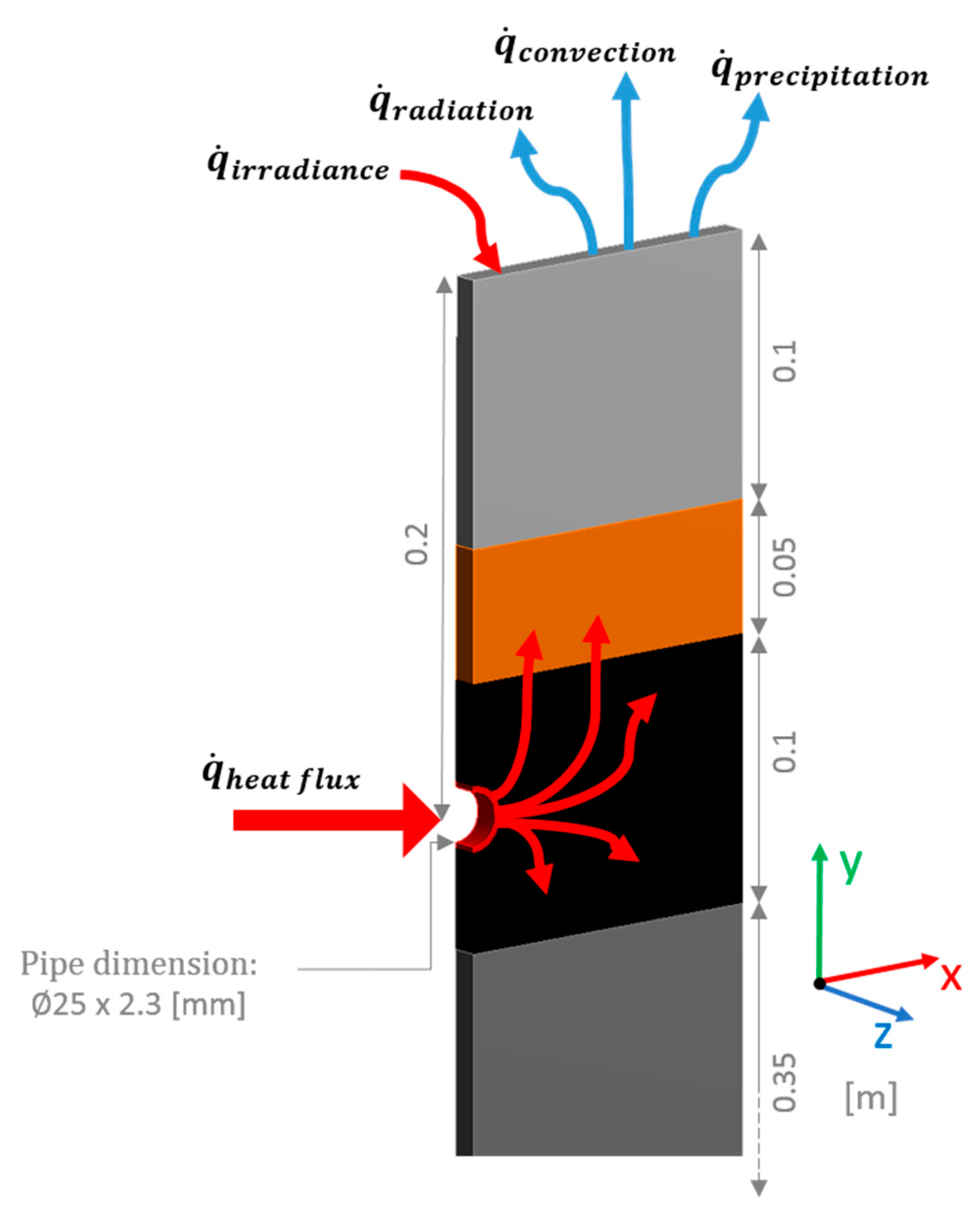
4.1. Parameters and Properties of the HPS Simulation Model

The HPS is simulated as a transient model. A time step of 15 min is used, in order to capture the fluctuant weather, as well as capturing the response time needed in an HPS to ensure good performance. Fifteen minutes is also an approximate value of the HPSs cycle time. A residual error of 1.0 e 4 (RMS level) is used in this study. The model includes the parameters:
  • Weather properties regarding temperature, precipitation, solar irradiation, and wind.
  • Material properties regarding density, thermal conductivity, and specific heat capacity.
  • Heat transfer equations regarding conductivity, convection, and radiation.
  • Operational parameters.
The construction of the HPS model is illustrated in Table 3 and, along with the material properties of the layers. Table 3 includes intervals for each value, which have been found in related literature. The surface layer A consists of the pavement which could be asphalt or, as in this study, paving stone. Layer B is a layer of rammed sand. The properties of layer C depend on the context of use. If the surface is regularly exposed to heavy loads of traffic, the normal material would be asphalt, as in this study. If the area serves as a walkway with minor loads, layer C could consist of rammed sand with embedded plastic PEX-pipes. Lastly, in layer E, there is a bearing layer of gravel or similar. In this study, plastic PEX-pipes have a spacing of 0.25 m. As a final note on the construction, Adl-Zarrabi et al. [28] conclude that the thermal properties of the material and spacing of the pipes have a large influence on the system’s performance, and the buried depth of the pipes are of less importance.
The final simulation model of the HPS is visualized in Figure 4. Symmetry, adiabatic conditions, and areal conversion equations are used to reduce the model size, which thus requires less computational power. The unstructured mesh grid used is based on proximity and curvature, containing 3936 elements. The simulation will predict heat transfer in the X- and Y-direction, as illustrated in Figure 4. Therefore, the boundary condition of the two surfaces in the Z-direction is set to be adiabatic. Also, symmetry is used on the surfaces in the X-direction. The bottom boundary condition is set to an average temperature of 9 °C, to reflect lower ground level in the urban area. The depth of the model is generous enough to not influence the result. The boundary conditions at the top surface of the model are presented in Equation (1), which includes convection, radiation, solar irradiance, and effects of precipitation. The heat transfer occurring by conduction is calculated in the model using the properties presented in Table 3.
The control strategy depends on sensors registering the temperature of the surface, T s u r f a c e , and controlling the power accordingly. As long as the outdoor temperature is below the starting temperature, the surface temperature, T s u r f a c e , is regulated relative to a set point temperature, T s e t   p o i n t . The set point temperature is either 2 °C as a standby mode during no precipitation, or 5 °C in an active mode in presence of precipitation. For example, the outdoor temperature may be −3 °C and precipitation is due in a couple of hours. Then the set point temperature will be set to 5°C well before the upcoming precipitation and then melt the snow fall, thus, preventing snow and ice formation on the pavement. The active mode refers to a preheat period of 4 h before precipitation and to when the surface is dry again after the precipitation. The control strategy, analyzing the difference between the surface temperature, T s u r f a c e , and the desired set point temperature, T s e t   p o i n t , determines the power applied by the HPS. The heat transfer occurring between the heat medium and the embedded pipes is expressed as power levels in the model, seen as q ˙ h e a t   f l u x in Figure 4. The levels range from 20 W/m2 to 160 W/m2, which corresponds to a range of 11 °C to 33 °C of the heat medium in the pipes. The control strategy is illustrated in Figure 5, both for times with no precipitation and in presence of precipitation. The HPS is only active at outdoor temperatures below 4 °C and the operational formula aims at keeping the temperature of the surface,   T s u r f a c e , above the set point temperature by a proactive approach to slow down the temperature drop as it approaches the set point temperature.
Equation (1) is the governing boundary condition on the top surface, including convection radiation, precipitation, and irradiance, as illustrated in Figure 4.
q ˙ s u r f a c e ( t ) = q ˙ i r r a d i a n c e q ˙ r a d i a t i o n q ˙ c o n v e c t i o n q ˙ p r e c i p i t a t i o n [ W / m 2 ] ,
where the four parameters of the equation are described in more detail in the following Equation (2)–(5). Equation (2) regards solar irradiance acting on the top surface.
q ˙ i r r a d i a n c e ( t ) = α · I ( t ) [ W / m 2 ] ,
where I ( t ) is the solar irradiance which are collected for Linköping from the data model STRÅNG, which is a mesoscale model for solar radiation [79]. α is the absorptivity of the surface, which is set to 0.2 in accordance with the literature presenting a range of 0.05 to 0.35 [80].
Equation (3) regards the radiation acting on the surface.
q ˙ r a d i a t i o n ( t ) = σ · ε · ( T s u r f a c e 4 ( t ) T a m b i e n t   a i r 4 ( t ) ) ,
where σ is the Stefan-Boltzmann constant. ε is the emissivity, which is set to 0.9 in accordance with the literature of urban surfaces ranging from 0.71 to 0.95 [81]. T s u r f a c e , is the temperature of the surface, which is measured in the simulation model. T a m b i e n t   a i r , is assumed to be the outdoor temperature, which is collected from the SMHIs open data and the weather station Malmslätt in Linköping, Sweden [70].
q ˙ c o n v e c t i o n ( t ) = h ( t ) · ( T s u r f a c e ( t ) T a m b i e n t   a i r ( t ) ) ,
where h is the heat transfer coefficient including Reynolds and Prandtl numbers and calculated in accordance with Çengel et al. [82], Holman [83], and Storck et al. [84]. The heat transfer coefficient is calculated at each time step of the simulation model and is dependent on the wind speed and temperature measurements collected from SMHIs open data and the weather station Malmslätt in Linköping, Sweden [70].
Equation (5) regards the precipitation, and if snowfall occurs, the snow’s sensible heat is first calculated. Secondly, the heat required to melt the snow is calculated and lastly, a calculation is made of the latent heat required to keep the ground surface at a constant temperature while the remaining precipitation is evaporated.
q ˙ p r e c i p i t a t i o n ( t ) = ρ w · n s ( t ) · ( c p , s · | 0   ° C T a i r ( t ) | + c m + ( 1 φ ) · c e ) / t ,
where ρ w is the density of water, which is set to be 1000 kg / m 3 [82], n s is the amount of precipitation collected from SMHI open data [70], c p , s is the specific heat capacity of snow and ice and set to 2110 J / kgK [82], c m is the melt enthalpy of water and is set to 333,700 J / kg [82], φ is the surface runoff factor and is set to 0.9, which is in range of the literature ranging between 0.7 and 0.95 for urban surfaces [85]. c e is the evaporation enthalpy of water, which is set to 2,500,000 J / kg [82]. t , is the time step of the model, which is 900 s (15 min) in this study.

Limitations and Comments on the Model

The model does not regard the choice of heat medium and electricity use of, e.g., pumps, since construction and use may differ significantly from one system to another. The properties stated in Table 3 may vary depending on moisture, porosity, potential air voids, and temperature of the material [76]. If the materials in the ground are at sub-zero temperatures, it can affect the thermal properties and increase energy use due to moisture transport in the ground, as analyzed by Xu and Tan [34]. However, as the HPS studied aims at drying the surface after precipitation and thereby minimize moisture, as well as keeping the ground layers above sub-zero temperatures, these issues are neglected in this study.
Regarding the boundary condition of the bottom surface, the surrounding ground often contains nearby infrastructure, such as storm drains, sewers or district heating pipes, which causes the average temperature of the ground to be higher than in rural areas. In addition to this, the HPS itself is an influencing factor when it turns on at 4 °C in the autumn, whereby normal cooling can never occur. The inertia of the ground causes the temperature to be higher lower into the ground than at the surface.
Moreover, Equations (1)–(5) represent parameters with the largest impact on HPS performance. Other parameters, such as dew or moisture on the surface, are neglected since the HPS aims to keep the surface warmer than the ambient air. Regarding Equation (2), the α-value of the pavement has a large impact on the affecting solar irradiance. In urban areas the surroundings will disturb irradiance, causing urban canyons [80] and making it difficult to assign a general α-value. When regarding radiation in Equation (3), the ambient temperature is considered to be that of the urban environment, as opposed to the sky temperature commonly used. However, during fully cloudy conditions the sky temperature may also be considered as the ambient temperature [35]. When snowfall occurs, the wind in Equation (4) acts on a surface film temperature of 0 °C regardless of the outdoor temperature. Moreover, during rainfall, the film temperature is assumed to be the same as the ambient temperature. Regarding Equation (5), the ground layers are considered to be impervious as it is desirable to keep the surface and ground layers dry. Moreover, urban areas often suffer heavy compaction due to demands for bearing capacity, which results in a reduced infiltration capacity [86]. Also, the temperature of the precipitation is assumed to be the same as the ambient temperature as it hits the top surface. The characteristics of snow vary, depending especially on whether the snow is uncompressed or compressed, with the latter requiring more energy to melt [87]. As the HPS starts to heat the ground four hours before predicted precipitation and aims to melt the snowflakes as they fall to the ground, the snow is considered to be uncompressed.
According to [1] the HPS should be designed to be able to keep the ground surface temperature at +5 °C when the air temperature is 5 °C higher than the design outdoor temperature, which is −16.6 °C for Linköping, Sweden [88]. Statistically, this means that a temporary snow cover will remain for no longer than two hours on five different occasions over a ten-year period. Statistically, snowfall of such intensity that snow cover will remain for more than eight hours occurs once every ten years.

4.2. Parameters and Properties of the DHC System’s Optimization Model

The DHC production in Linköping is based on the incineration plants: The Gärstad waste-fueled CHP plant, located in the northern part of Linköping, and a mixed-fueled CHP plant located in the central part. The system is complemented with a biomass-fueled CHP plant and a heat-only boiler (HOB) using biomass in the nearby town of Mjölby. As a backup, there are also heat-only boilers using oil and electricity to cover peak demand. The model of the studied DHC system is visualized in Figure 6, and the basic input data for the utilities is presented in Table 4. The DHC system and optimization model has been studied previously by Blomqvist et al. [89].
The Gärstad CHP plant consists of three waste incineration boilers, illustrated as CHP 1–3, 4, and 5 in Figure 6. They are hybrid systems, with flue gas condensing and steam turbine through a gas turbine heat recovery steam generator. CHP 1–3 has a maximum capacity of 75 MW heat, with an additional 15 MW heat from flue gas condensing and 10 MW electricity. CHP 4 has a steam turbine capacity of 68 MW heat, and an additional 15 MW heat from flue gas condensing and 19 MW electricity. CHP 5 has a steam turbine capacity of 84 MW, and an additional 12 MW heat from flue gas condensing and 21 MW electricity. The central CHP plant consists of three boilers and three steam turbines, where two are backpressure turbines, and one combined condensing and backpressure turbine. The first boiler is fueled with coal, with fractions of rubber. The second boiler uses heating oil. The third boiler, with flue gas condensing, is fueled with biomass made from wood products and fractions of plastics. The central plant can produce electricity and heat or use a direct condenser for the sole production of heat. Cooling of the condensing turbine is achieved using water from the nearby river Stångån, resulting in 50 GWh heat potentially being wasted in Stångån annually. The technical input data may be seen in Table 4.
The district cooling in the system is produced in an absorption plant with a capacity of 12 MW cooling using heat from the DHC system and an electricity-powered compression-cooling plant with a capacity of 6 MW cooling.
In order to calculate the local GHG emissions, the factors presented in Table 5 are used. The locally emitted GHG is a result of the fuel use in the DHC system. The biomass consists of primary and secondary wood fuels. The majority of household waste is organic and comes from the surrounding region. The subsequent effects on the global GHG emissions are calculated and analyzed by using three different factors, also presented in Table 5. The factors are of Swedish electricity mix, Nordic electricity mix, and electricity produced by coal condensing plants. The effects on the global GHG emissions are caused by the local changes in electricity production from the CHP plants and the use of biomass, which is seen as a scarce resource in this study.

5. Results

The results in the paper include three sections, (1) where the two models of the HPS and DHC system will be compared to actual system performance from 2016, and (2) where the overall performance of the HPS will be analyzed. In the third (3) section the impact of the HPS on the DHC system will be analyzed.

5.1. Comparing Models of the HPS and DHC System to Actual System Performance

Simulation of the HPS model is compared to annual and monthly statistical data for the winter months, Jan–Apr and Oct–Dec 2016. In Figure 7, the result of the reference Scenario R is presented together with the statistical data. The simulation model generates an annual difference of 2%, and a monthly maximum difference of 10%, except during the low use months of April and October. Moreover, the operational hours of the reference scenario are 3055 h, compared with 3041 h at temperatures below the starting temperature of 4 °C, as presented in Table 2. The small difference is due to modeling issues. The model time step of 15 min has a higher resolution than the hourly statistical data and causes parts of an hour to count when the outdoor temperature fluctuates around the starting temperature of 4 °C.
The fuel use of reference Scenario R from the optimization model in MODEST is compared to statistics as visualized in Figure 8. The total annual fuel use differs by 5%, with the optimization model resulting in energy use of 2440 GWh and the statistics showing 2323 GWh.

5.2. Performance of the HPS and Energy Use of the Studied Scenarios

Figure 9 shows the performance of the HPS in the studied scenarios during January and February of 2016. The temperature of the top surface in the scenarios is displayed along with outdoor temperature and precipitation. A rapid decrease in the surface temperature indicates precipitation, as the surface in the simulation receives large negative power, in accordance with boundary Equation (5).
The energy use of scenarios R, 1 and 2 is presented in Figure 10. The annual energy use of the studied scenarios amounts to 6.3 GWh for Scenario R, 5.6 GWh for Scenario 1, and 4.5 GWh for Scenario 2, generating a potential energy saving of 28%. Moreover, the results correspond to an average annual use 180 kWh/m2 for Scenario R, 161 kWh/m2 for Scenario 1, and 129 kWh/m2 for Scenario 2.
A duration diagram of the HPS is presented in Figure 11. Savings are made in all the power steps, and the average energy use ranges from 57.5 W/m2 to 49.7 W/m2, corresponding to a potential energy saving of 14% between the scenarios. The operational hours of the scenarios differ by 500 h, ranging from 3055 h to 2525 h.

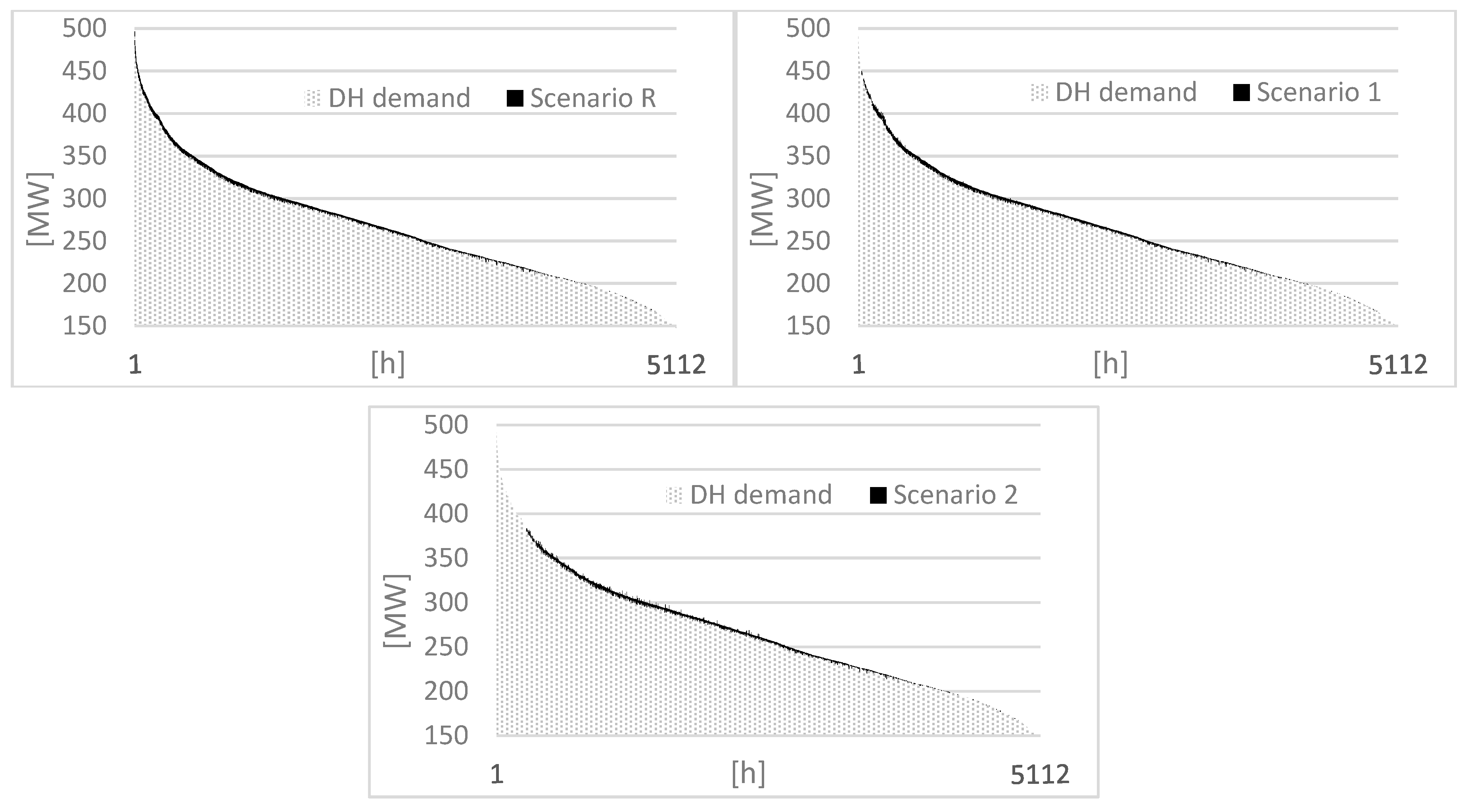
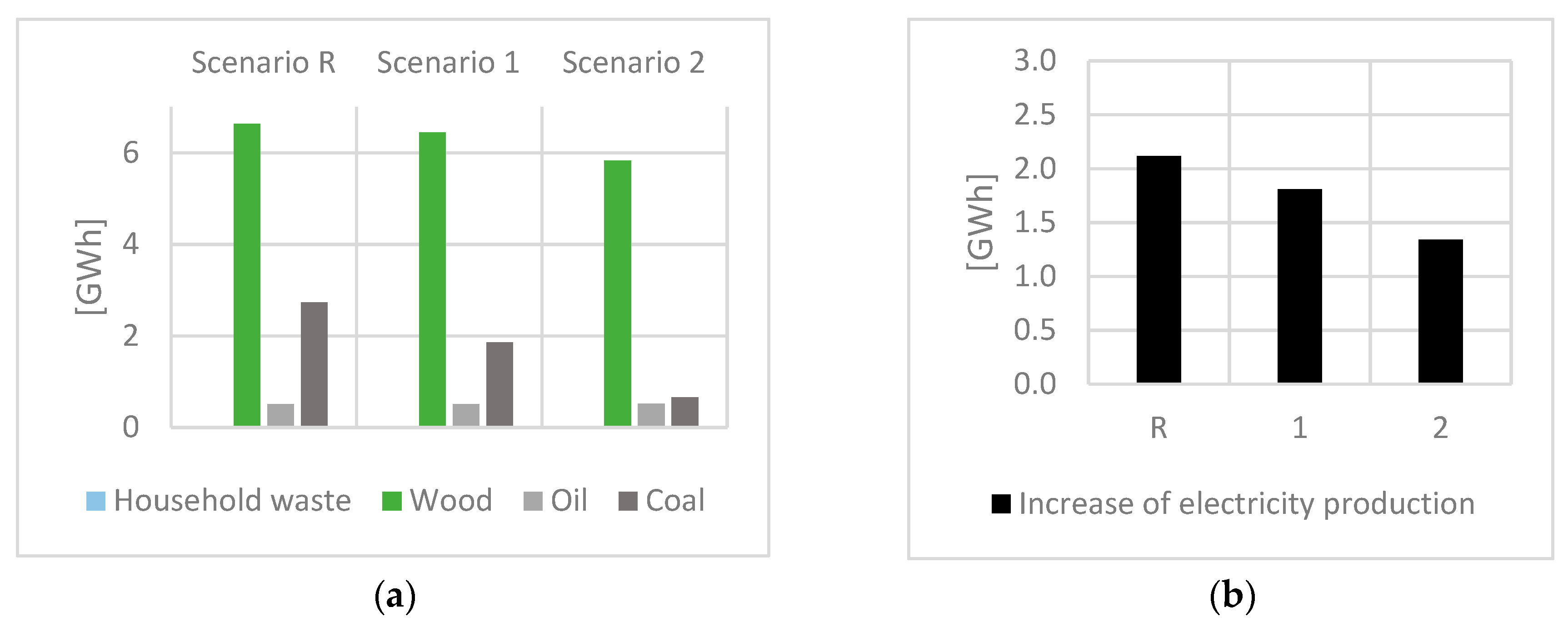
5.3. Evaluation of the Impact the HPS Has on the DHC System

The primary energy use of the DHC system is presented in Figure 12. Household waste is the main source, followed by biomass. Coal is needed in the peak 1000 h, and at a production level of 375 MW the HOB using biomass is needed, while oil is required once the production level exceeds 400 MW.
Figure 13 shows the time of operation of the HPS and how it coincides with the demand in the DHC system. For the reference Scenario R, the time of operation coincides with the peak demand in the DHC system. Scenario 1 is excluded from the top days of the peak demand, approximately 50 h. Furthermore, Scenario 2 is excluded from the top weeks, approximately 300 h.
Figure 14a presents the primary energy savings of each scenario, while Figure 14b shows the increase in electricity production due to increased production at the CHP plants. It is worth noting that mostly renewable resources such as biomass are used for the HPS and that electricity production increases as the use of HPS increases.
Figure 15 presents the increase in local emissions and decrease in global emissions. The local emissions increase in all scenarios, as a result of increased production in the DHC system. The local emissions amount to 34 kgCO2, eq/m2 for Scenario R, 25 kgCO2, eq/m2 for Scenario 1, and 13 kgCO2, eq/m2 for Scenario 2. Including the operational hours of the studied system, the value could be expressed as 11 gCO2, eq/m2, h for Scenario R, 9 gCO2, eq/m2, h for Scenario 1, and 5 gCO2, eq/m2, h for Scenario 2. As presented in Figure 15, global emissions are reduced in all scenarios, mostly due to the increased production of electricity in the CHP plants, as presented in Figure 14b. Moreover, reduced use of the scarce resource of biomass has a positive impact on global GHG emissions.

6. Discussion

6.1. The Scenarios and Modeling of the HPS

For scenarios 1 and 2, the heat medium should have freeze protection, or the HPS should have an idling mode where the medium is kept above freezing and circulating in the pipes. The model is constrained to a maximum power of 160 W/m2, which is lower than the theoretical design power for the geographical location stated in 1976 [1], but in line with other more recent literature [7,78]. The maximum power corresponds to 33 °C, which enables the use of the return water in the DHC system. Besides being able to operate an HPS, the opportunity to decrease the return temperature can result in a more efficient DHC system, as it increases the output of the flue gas condensation, as argued in the introduction.
It should be noted that, overall, the studied year was warmer than a normal year. However, January of 2016 was colder, as were October and November. For 3041 h during the studied months, the temperature dropped below 4°C, which is the temperature at which the HPS becomes active. In terms of precipitation, the studied year was dryer than the normalized year. October is the only month when the precipitation was above normal. The cold month of January, in particular, had less precipitation than the normalized data. This is in line with the ideas of the scenario, with shutdown periods at lower temperatures, since the air’s saturation level decreases at lower temperatures, which, in turn, reduces the occurrence of precipitation.
The simulation model of the HPS shows good agreement with measurements. The difference between the annual averaged model prediction and the actual performance was 2%, and the monthly difference was below 10% for the cold winter months. A higher relative average was only found for April and October when the system was only scarcely used. The comparison was applied to an HPS area of 33,000m2, due to imperfect data from one subsystem at the time of the study. This is the reason why Figure 7 shows lower energy use than reference Scenario R in Figure 10. The optimization model of the DHC system in MODEST resulted in an annual difference of 5% and good agreement in terms of allocation of the primary energy sources.

6.2. Performance of the HPS

In order to analyze the performance of the HPS, it is stated that the HPS should be designed to keep the surface temperature at +5 °C when the air temperature is 5 °C higher than the design outdoor temperature [1]. In Figure 9, reference Scenario R indicates that it is possible to achieve this, as the surface temperature is above 0 °C when the outdoor temperature is −11 °C. The temperature set point in the model is 2 °C, but as the model includes cooling effects from wind, radiation, and precipitation, it is possible to keep a lower temperature setting than 5 °C. Moreover, the air is dry at these low temperatures and in combination with the surface temperature always being higher than the that of the air, the risk of a slippery surface is minimized. It comes down to a choice between keeping the surface above freezing at all times or settling for minimizing the risk of slipping, in relation to efficient energy use.
In Figure 9, which presents the performance of the HPS, a rapid decrease in the surface temperature indicates precipitation, as the surface in the simulation receives negative power derived from Equation (5). The temperature increases quickly as an indication of the HPS reacting to the precipitation. Looking more closely at Scenario 2 in January, one can see a large drop in temperature. The drop is explained by that the system is turned off and prolonged precipitation, in the form of snow, falls when the outdoor temperature increases from low levels. This indicates that the snow will remain on the surface, whereas the snow will be melted in Scenario 1, as the temperature climbs above 0 °C. This poses a design question of how many hours the HPS is allowed to fail and still be seen as acceptable, which can be decided upon the desired function of the system and location. Moreover, during late February, the large temperature variation is explained by the spring sun.

6.3. The impact of the HPS on the DHC System

The largest change in energy use between the scenarios is seen in the cold month of January, as shown in Figure 10. In connection to the duration diagram in Figure 11, where the operational hours of the peak power 160 W/m2 are decreasing, it is concluded that the pickup loads after shutdown periods in scenarios 1 and 2 do not result in the HPS demanding more peak power than the reference Scenario R. However, as presented in Figure 9, on the days around 10 January, the performance of the scenario may enable snowfall to remain on the surface, resulting in poor performance of the HPS in Scenario 2. This indicates that an HPS that shuts down at a temperature of −5 °C or lower performs poorly but presents good energy performance values. However, Scenario 1, when the HPS shuts down at a temperature of −10 °C or lower, presents good performance and also reduced the energy use of 3 W/m2 (5%) for average use or 640 MWh (10%) for annual energy use, compared to the reference Scenario R. Moreover, Scenario 1 is excluded from the top 50 h regarding peak demand in the DHC system, as presented in Figure 13, which in turn reduces the use of fossil fuel, as seen in Figure 14a. In addition, Scenario 1 reduces local GHG emissions by 25% relative to the reference Scenario R. However, Scenario 1 also results in less electricity generated at the CHP plants relative to Scenario R, leading to less available electricity on the market. This, in turn, leads to a reduced positive effect on global GHG emissions.
The local emissions in this study only include the use of HPS and not the alternative use of conventional snow clearance using heavy machinery. However, the literature points to the HPS being the more GHG efficient alternative, indicating reduced local emissions if a comparison were to be made. The HPS generates a low value of 11 gCO2, eq/m2, h for the reference Scenario R. In a future fossil-free DHC system, the local GHG emissions from the HPS will decrease even more.
The factor to analyze at implementation is the time it takes for the HPS to produce a sufficient temperature at the surface to minimize the risk of slipperiness, at times when the temperature rises from below −10 °C in conjunction with precipitation shortly thereafter.

7. Conclusions

  • The study indicates that the HPS is suitable for the use of return temperatures in a DHC system. An HPS could further decrease the return temperature, thereby potentially increasing the efficiency of the DHC system. Furthermore, in a future DHC system with lower supply temperatures, it is also desirable to achieve lower return temperatures to maintain an efficient DHC system.
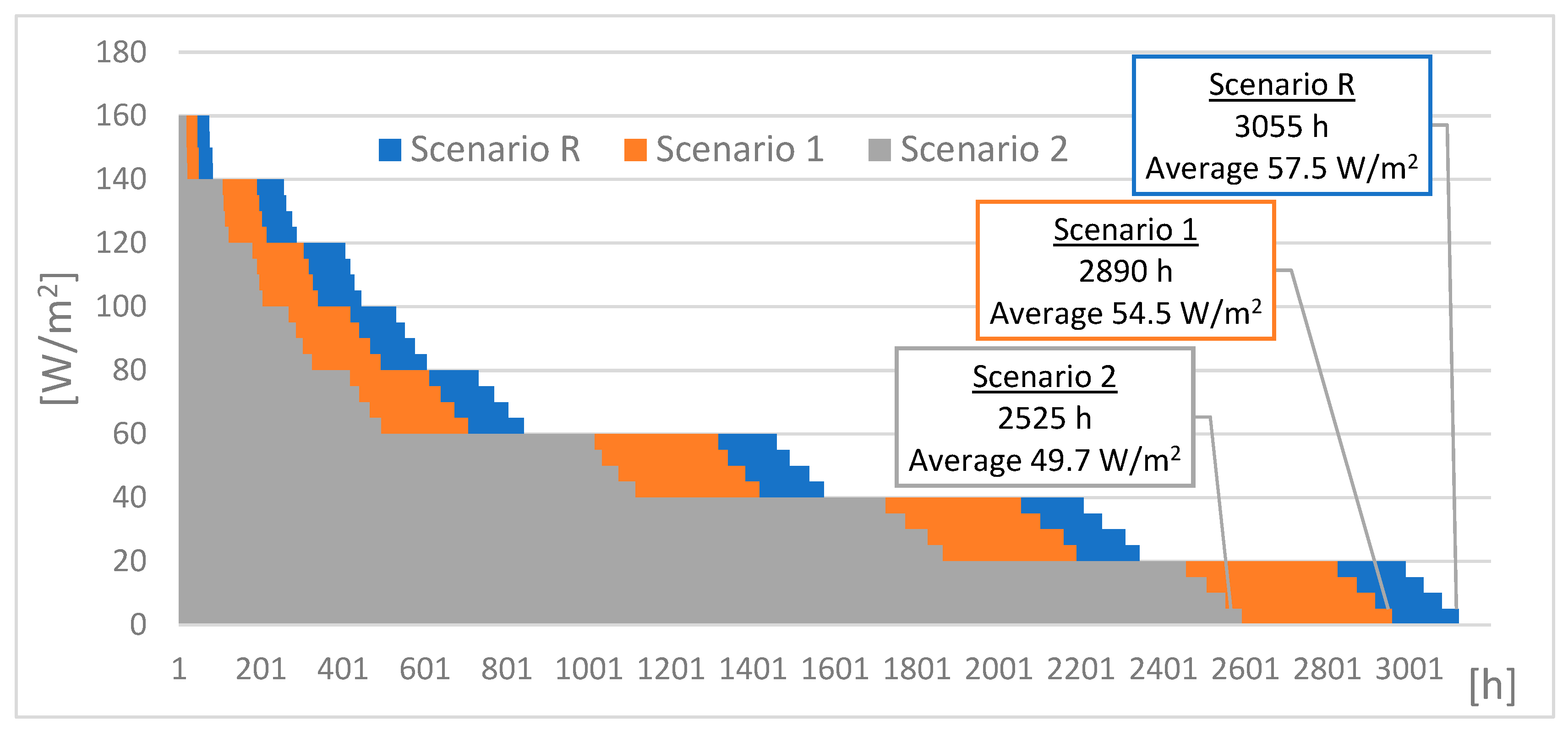
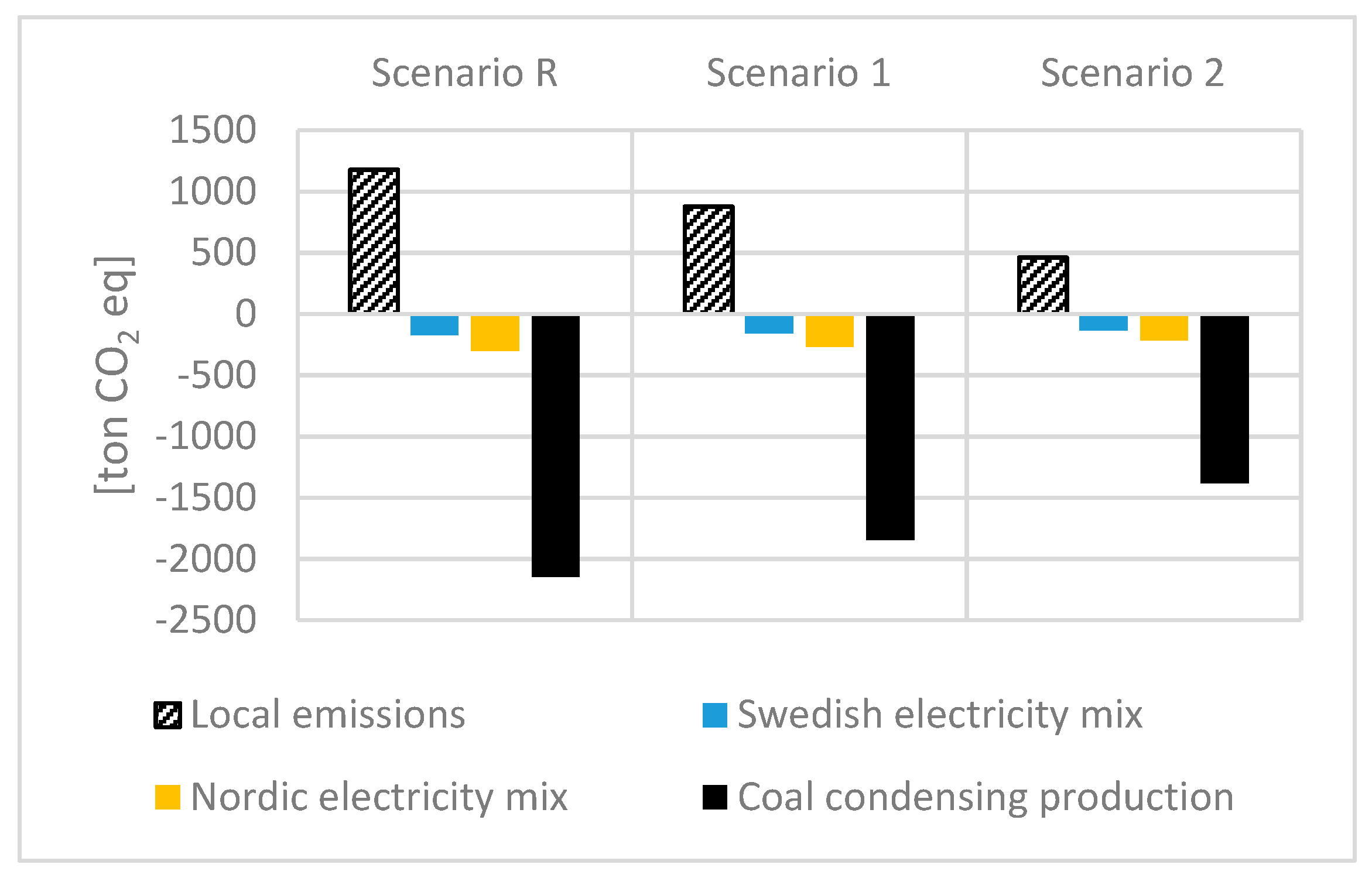
  • A control strategy that shuts down the HPS at temperatures below −10 °C results in a 10% energy saving, avoidance of use during the top 50 h of peak demand in the DHC system, reduced use of fossil fuel and a 25% reduction in local GHG emissions, whilst maintaining sufficient performance of the HPS.
  • Utilizing HPS connected to a DHC system which has CHP can potentially result in increased electricity production. This generates a positive effect and reduction on the global GHG emissions if a coal condensing power plant is regarded as the marginal production unit in the European electricity market. In a future fossil-free production of DHC, the generated electricity will fully derive from renewable resources. This will improve the impact an HPS has on the GHG emissions even further.

Author Contributions

Conceptualization, S.B., P.R. and L.Ö.; data curation, S.B.; formal analysis, S.B.; funding acquisition, L.Ö.; investigation, S.B.; methodology, S.B.; project administration, S.B. and P.R.; software, S.B. and S.A.; supervision, P.R. and L.Ö.; validation, S.B.; visualization, S.B.; writing—original draft, S.B., S.A. and P.R.; writing—review & editing, S.B.

Funding

This study has been financed by the Swedish Agency for Economic and Regional Growth and the energy companies Tekniska verken AB and E.ON Sweden AB, as well as the housing companies Stångåstaden AB, AB Lejonfastigheter, Fastighets AB L E Lundberg, and Akademiska Hus AB.

Acknowledgments

The authors gratefully acknowledge Tekniska verken AB, for its insights and information regarding the HPS and DHC system.

Conflicts of Interest

The authors declare no conflict of interest.

References

  1. Byggnadsstyrelsen. Markvärme; KBS Rapport; Byggnadsstyrelsen: Stockholm, Sweden, 1976. [Google Scholar]
  2. Lund, J.W.; Boyd, T.L. Geothermal direct-use in the United States update: 1995–1999. In Proceedings of the Proceedings World Geothermal Congress 2000, Tohoku, Japan, 28 May–10 June 2000; Geo-Heat Center, Oregon Institute of Technology Klamath Falls: Kyushu, Japan, 2000; pp. 297–305. [Google Scholar]
  3. Lund, J.W. Reconstruction of a pavement geothermal deicing system. Geo-Heat Cent. Q. Bull. 1999, 20, 14–17. [Google Scholar]
  4. American Society of Heating, Refrigerating and Air-Conditioning Engineers. 2011 ASHRAE Handbook: Heating, Ventilating, and Air-Conditioning Applications; ASHRAE: Atlanta, GA, USA, 2011; ISBN 9781936504077. [Google Scholar]
  5. Mensah, K.; Choi, J.M. Review of technologies for snow melting systems. J. Mech. Sci. Technol. 2015, 29, 5507–5521. [Google Scholar] [CrossRef]
  6. Pan, P.; Wu, S.; Xiao, Y.; Liu, G. A review on hydronic asphalt pavement for energy harvesting and snow melting. Renew. Sustain. Energy Rev. 2015, 48, 624–634. [Google Scholar] [CrossRef]
  7. Lund, J.W.; Boyd, T.L. Direct utilization of geothermal energy 2015 worldwide review. Geothermics 2016, 60, 66–93. [Google Scholar] [CrossRef]
  8. Zwarycz, K. Snow Melting and Heating Systems Based on Geothermal Heat Pumps at Goleniow Airport, Poland; The United Nations University, Geothermal training programme: Reykjavik, Iceland, 2002. [Google Scholar]
  9. Shen, W.; Ceylan, H.; Gopalakrishnan, K.; Kim, S.; Taylor, P.C.; Rehmann, C.R. Life cycle assessment of heated apron pavement system operations. Transp. Res. Part D Transp. Environ. 2016, 48, 316–331. [Google Scholar] [CrossRef]
  10. Shen, W.; Gopalakrishnan, K.; Kim, S.; Ceylan, H. Assessment of Greenhouse Gas Emissions from Geothermal Heated Airport Pavement System. ISSN Int. J. Pavement Res. Technol. Int. J. Pavement Res. Technol. 1997, 88, 233–242. [Google Scholar]
  11. Shen, W.; Ceylan, H.; Gopalakrishnan, K.; Kim, S.; Nahvi, A. Sustainability Assessment of Alternative Snow-Removal Methods for Airport Apron Paved Surfaces; Federal Aviation Administration: Atlantic City, NJ, USA, 2017.
  12. Chi, Z.; Yiqiu, T.; Fengchen, C.; Qing, Y.; Huining, X. Long-term thermal analysis of an airfield-runway snow-melting system utilizing heat-pipe technology. Energy Convers. Manag. 2019, 186, 473–486. [Google Scholar] [CrossRef]
  13. Zhang, N.; Yu, X.; Li, T. Numerical Simulation of Geothermal Heated Bridge Deck. In Proceedings of the International Conference on Transportation Infrastructure and Materials (ICTIM 2017), Qingdao, China, 9–12 June 2017. [Google Scholar]
  14. Yu, X.; Zhang, N.; Pradhan, A.; Puppala, A.J. Geothermal Energy for Bridge Deck and Pavement Deicing—A Brief Review. In Proceedings of the Geo-Chicago 2016, Chicago, IL, USA, 14–18 August 2016; American Society of Civil Engineers: Reston, VA, USA, 2016; pp. 598–609. [Google Scholar]
  15. Swedish Energy Agency Annual Energy Statistics (Electricity, Gas and District Heating). Available online: http://www.scb.se/en0105-en (accessed on 18 April 2019).
  16. Gunnlaugsson, E.; Reykjavikur Baejarhals, O. District heating in Reykjavík; past–present–future. In Proceedings of the 30th Anniversary Workshop, Reykjavík, Iceland, 26 August 2008. [Google Scholar]
  17. Solaimanian, M.; Kennedy, T.W. Predicting Maximum Pavement Surface Temperature Using Maximum Air Temperature and Hourly Solar Radiation. Transp. Res. Rec. 1993, 1417, 1–11. [Google Scholar]
  18. Gustavsson, T.; Bogren, J.; Green, C. Road Climate in Cities:A Study of the Stockholm Area, South-East Sweden. Meteorol. Appl. 2001, 8, 481–489. [Google Scholar] [CrossRef]
  19. Andriopoulou, S. A Review on Energy Harvesting from Roads; [TSC-MT 12-017]; KTH Royal Institute of Technology: Stockholm, Sweden, 2012. [Google Scholar]
  20. National Research Council (US). Comparing Salt and Calcium Magnesium Acetate; National Research Council: Washington, DC, USA, 1991. [Google Scholar]
  21. Amrhein, C.; Strong, J.E.; Mosher, P.A. Effect of deicing salts on metal and organic matter mobilization in roadside soils. Environ. Sci. Technol. 1992, 26, 703–709. [Google Scholar] [CrossRef]
  22. Bäckström, M.; Karlsson, S.; Bäckman, L.; Folkeson, L.; Lind, B. Mobilisation of heavy metals by deicing salts in a roadside environment. Water Res. 2004, 38, 720–732. [Google Scholar] [CrossRef] [PubMed]
  23. Fischel, M. Evaluation of Selected Deicers Based on a Review of the Literature; Colorado Department of Transportation: Denver, CO, USA, 2001.
  24. Howard, K.W.F.; Haynes, J. Groundwater Contamination due to Road De-icing Chemicals - Salt Balance Implications. Geosci. Can. 1993, 20, 1–8. [Google Scholar]
  25. Kroening, S.; Ferrey, M. The Condition of Minnesota’s Groundwater, 2007–2011; Minnesota Pollution Control Agency: Saint Paul, MI, USA, 2013.
  26. Fay, L.; Shi, X. Environmental Impacts of Chemicals for Snow and Ice Control: State of the Knowledge. Water Air Soil Pollut. 2012, 223, 2751–2770. [Google Scholar] [CrossRef]
  27. Nevalainen Henaes, H. Impact on Society from Conventional Winter Road Maintenance and Ground Heating (sv: Samhällspåverkan vid Konventionell Vinterväghållning och Markvärme); Lunds University—Faculty of Engineering: Lund, Sweden, 2018. [Google Scholar]
  28. Adl-Zarrabi, B.; Mirzanamadi, R.; Johnsson, J. Hydronic pavement heating for sustainable ice-free roads. Transp. Res. Procedia 2016, 14, 704–713. [Google Scholar] [CrossRef]
  29. Nixon, W.A. Improved Cutting Edges for Ice Removal; Strategic Highway Research Program: Washington, DC, USA, 1993. [Google Scholar]
  30. Schyllander, J. Fotgängarolyckor: Statistik och Analys; Swedish Civil Contingencies Agency: Karlstad, Sweden, 2014.
  31. Carlsson, A.; Sawaya, B.; Kovaceva, J.; Andersson, M. Skadereducerande Effekt av Uppvärmda Trottoarer, Gång- och Cykelstråk (TRV 2016/19843); Chalmers University of Technology: Gothenburg, Sweden, 2018. [Google Scholar]
  32. Öberg, G.; Arvidsson, A.K. Injured Pedestrians: The Cost of Pedestrian Injuries Compared to Winter Maintenance Costs; Swedish National Road and Transport Research Institute: Linköping, Sweden, 2012.
  33. Mattsson, A. Samhällsekonomiska Effekter av VinterväGhåLlning för GåEnde.: En Kostnads–Nyttoanalys av VinterväGhåLlning och GåNgtrafikanters Singelolyckor i Stockholms Stad; Linköping University: Linköping, Sweden, 2017. [Google Scholar]
  34. Xu, H.; Tan, Y. Modeling and operation strategy of pavement snow melting systems utilizing low-temperature heating fluids. Energy 2015, 80, 666–676. [Google Scholar] [CrossRef]
  35. Mirzanamadi, R. Ice Free Roads Using Hydronic Heating Pavement with Low Temperature Thermal Properties of Asphalt Concretes and Numerical Simulations; Chalmers University of Technology: Gothenburg, Sweden, 2017. [Google Scholar]
  36. Rees, S.J.; Spitler, J.D.; Xiao, X. Transient analysis of snow-melting system performance. ASHRAE Trans. 2002, 108 Pt 2, 406–423. [Google Scholar]
  37. Commission of the European communities. 20 20 by 2020 Europe’s Climate Change Opportunity; Commission of the European Communities: Brussels, Belgium, 2008. [Google Scholar]
  38. Reinfeldt, F.; Olofsson, M. Prop. 2008/09:163: En Sammanhållen Klimat- och Energipolitik; Government Office: Stockholm, Sweden, 2008. [Google Scholar]
  39. Löfven, S.; Baylan, I. Prop. 2017/18:228: Energipolitikens inriktning; Government Office: Stockholm, Sweden, 2018. [Google Scholar]
  40. Fossil free Sweden (sv: Fossilfritt Sverige). Roadmaps for Fossil Free Competitiveness—The Heating Sector (sv: Färdplan för Fossilfri Konkurrenskraft—Uppvärmningsbranschen); Fossil Free Sweden: Stockholm, Sweden, 2018. [Google Scholar]
  41. Kim, H.-J.; Yu, J.-J.; Yoo, S.-H.; Kim, H.-J.; Yu, J.-J.; Yoo, S.-H. Does Combined Heat and Power Play the Role of a Bridge in Energy Transition? Evidence from a Cross-Country Analysis. Sustainability 2019, 11, 1035. [Google Scholar] [CrossRef]
  42. Lake, A.; Rezaie, B.; Beyerlein, S. Review of district heating and cooling systems for a sustainable future. Renew. Sustain. Energy Rev. 2017, 67, 417–425. [Google Scholar] [CrossRef]
  43. Sayegh, M.A.; Danielewicz, J.; Nannou, T.; Miniewicz, M.; Jadwiszczak, P.; Piekarska, K.; Jouhara, H. Trends of European research and development in district heating technologies. Renew. Sustain. Energy Rev. 2016, 68, 1183–1192. [Google Scholar] [CrossRef]
  44. Lund, R.; Mathiesen, B.V. Large combined heat and power plants in sustainable energy systems. Appl. Energy 2015, 142, 389–395. [Google Scholar] [CrossRef]
  45. Stankeviciute, L.; Krook Riekkola, A. Assessing the development of combined heat and power generation in the EU. Int. J. Energy Sect. Manag. 2014, 8, 76–99. [Google Scholar] [CrossRef]
  46. Werner, S. International review of district heating and cooling. Energy 2017, 137, 617–631. [Google Scholar] [CrossRef]
  47. Sernhed, K.; Lygnerud, K.; Werner, S. Synthesis of recent Swedish district heating research. Energy 2018, 151, 126–132. [Google Scholar] [CrossRef]
  48. Djuric Ilic, D.; Dotzauer, E.; Trygg, L.; Broman, G. Introduction of large-scale biofuel production in a district heating system e an opportunity for reduction of global greenhouse gas emissions. J. Clean. Prod. 2014, 64, 552–561. [Google Scholar] [CrossRef]
  49. Helin, K.; Zakeri, B.; Syri, S.; Helin, K.; Zakeri, B.; Syri, S. Is District Heating Combined Heat and Power at Risk in the Nordic Area?—An Electricity Market Perspective. Energies 2018, 11, 1256. [Google Scholar] [CrossRef]
  50. Gadd, H.; Werner, S. Achieving low return temperatures from district heating substations. Appl. Energy 2014, 136, 59–67. [Google Scholar] [CrossRef] [Green Version]
  51. Lauenburg, P. Temperature optimization in district heating systems. Adv. Dist. Heat. Cool. Syst. 2016, 223–240. [Google Scholar] [CrossRef]
  52. Frederiksen, S.; Werner, S. District Heating and Cooling, 1st ed.; Studentlitteratur: Lund, Sweden, 2013; ISBN 9789144085302. [Google Scholar]
  53. Lund, H.; Werner, S.; Wiltshire, R.; Svendsen, S.; Thorsen, J.E.; Hvelplund, F.; Mathiesen, B.V. 4th Generation District Heating (4GDH): Integrating smart thermal grids into future sustainable energy systems. Energy 2014, 68, 1–11. [Google Scholar] [CrossRef]
  54. ANSYS Inc. ANSYS® WorkbenchTM, Release 18.0.; ANSYS® CFX®, ANSYS Inc.: Canonsburg, PA, USA, 2016. [Google Scholar]
  55. Division of Energy System at Linköping University. Converter; Linköping University: Linköping, Sweden, 2016. [Google Scholar]
  56. Henning, D. MODEST for Windows; IEI Energy Systems; Linköping University: Linköping, Sweden, 2014. [Google Scholar]
  57. Temam, R. Navier-Stokes Equations: Theory and Numerical Analysis; AMS Chelsea Pub: Amsterdam, The Netherlands, 2001; ISBN 0821827375. [Google Scholar]
  58. ANSYS Inc. ANSYS Documentation Release 18.0; ANSYS Inc.: Canonsburg, PA, USA, 2016. [Google Scholar]
  59. Henning, D. MODEST—An energy-system optimisation model applicable to local utilities and countries. Energy 1997, 22, 1135–1150. [Google Scholar] [CrossRef]
  60. Henning, D. Optimisation of Local and National Energy Systems: Development and Use of the MODEST Model; Division of Energy Systems, Department of Mechanical Engineering, Linköpings University: Linköping, Sweden, 1999; ISBN 9172193921. [Google Scholar]
  61. Åberg, M.; Widén, J.; Henning, D. Sensitivity of district heating system operation to heat demand reductions and electricity price variations: A Swedish example. Energy 2012, 41, 525–540. [Google Scholar] [CrossRef]
  62. Åberg, M.; Henning, D. Optimisation of a Swedish district heating system with reduced heat demand due to energy efficiency measures in residential buildings. Energy Policy 2011, 39, 7839–7852. [Google Scholar] [CrossRef]
  63. Lidberg, T.; Olofsson, T.; Trygg, L. System impact of energy efficient building refurbishment within a district heated region. Energy 2016, 106, 45–53. [Google Scholar] [CrossRef]
  64. Henning, D.; Trygg, L. Reduction of electricity use in Swedish industry and its impact on national power supply and European CO2 emissions. Energy Policy 2008, 36, 2330–2350. [Google Scholar] [CrossRef]
  65. Sundberg, G.; Orgen, J.; Odin, S. Project financing consequences on cogeneration: Industrial plant and municipal utility co-operation in Sweden. Energy Policy 2003, 31, 491–503. [Google Scholar] [CrossRef]
  66. Gebremedhin, A. The role of a paper mill in a merged district heating system. Appl. Therm. Eng. 2003, 23, 769–778. [Google Scholar] [CrossRef]
  67. Lund, R.; Ilic, D.D.; Trygg, L. Socioeconomic potential for introducing large-scale heat pumps in district heating in Denmark. J. Clean. Prod. 2016, 139, 219–229. [Google Scholar] [CrossRef] [Green Version]
  68. Amiri, S.; Henning, D.; Karlsson, B.G. Simulation and introduction of a CHP plant in a Swedish biogas system. Renew. Energy 2013, 49, 242–249. [Google Scholar] [CrossRef]
  69. Blomqvist, S.; Nyberg, S.; Energisystem, A. Modellering och Energieffektivisering av Befintligt Markvärmesystem; Linköping University: Linköping, Sweden, 2014. [Google Scholar]
  70. Swedish Meteorological and Hydrological Institutes SMHI’s Open Data. Available online: https://www.smhi.se/en/services/open-data/search-smhi-s-open-data-1.81004 (accessed on 14 March 2019).
  71. Hassn, A.; Chiarelli, A.; Dawson, A.; Garcia, A. Thermal properties of asphalt pavements under dry and wet conditions. Mater. Des. 2016, 91, 432–439. [Google Scholar] [CrossRef]
  72. Li, H.; Harvey, J.; Jones, D. Multi-dimensional transient temperature simulation and back-calculation for thermal properties of building materials. Build. Environ. 2013, 59, 501–516. [Google Scholar] [CrossRef]
  73. Shin, A.H.; Kodide, U. Thermal conductivity of ternary mixtures for concrete pavements. Cem. Concr. Compos. 2012, 34, 575–582. [Google Scholar] [CrossRef]
  74. Ohemeng, E.A.; Yalley, P.P.-K. Models for predicting the density and compressive strength of rubberized concrete pavement blocks. Constr. Build. Mater. 2013, 47, 656–661. [Google Scholar] [CrossRef]
  75. Ižvolt, L.; Dobeš, P. Test Procedure Impact for the Values of Specific Heat Capacity and Thermal Conductivity Coefficient. Procedia Eng. 2014, 91, 453–458. [Google Scholar] [CrossRef] [Green Version]
  76. Sundberg, J. Thermal Properties of Soil and Rock (sv: Termiska Egenskaper i jord och Berg); Swedish Geotechnical Institute (SGI): Linköping, Sweden, 1991; Volume 12. [Google Scholar]
  77. Luca, J.; Mrawira, D. New Measurement of Thermal Properties of Superpave Asphalt Concrete. J. Mater. Civ. Eng. 2005, 17, 72–79. [Google Scholar] [CrossRef]
  78. Uponor Uponor surface heating system (sv: Uponor ytvärmesystem). Heating, Ventilation and Sanitation Manual; Uponor AB: Västerås, Sweden, 2018; pp. 547–565. [Google Scholar]
  79. Swedish Meteorological and Hydrological Institute; Swedish Radiation Safety Authority; Swedish Environmental Protection Agency STRÅNG. A Mesoscale Model for Solar Radiation. Available online: http://strang.smhi.se/ (accessed on 26 April 2019).
  80. Santamouris, M. (Matheos) Energy and Climate in the Urban Built Environment—Chapter 11 Appropiate Materials for the Urban Environment; Santamouris, M., Ed.; James & James: Athens, Greece, 1999; ISBN 9781873936900. [Google Scholar]
  81. Brown, R.D.; Gillespie, T.J. Microclimatic Landscape Design: Creating Thermal Comfort and Energy Efficiency; J. Wiley & Sons: Guelph, ON, Canada, 1995; ISBN 0471056677. [Google Scholar]
  82. Çengel, Y.A.; Turner, R.H.; Cimbala, J.M. Fundamentals of Thermal-Fluid Sciences; McGraw Hill Higher Education: New York, NY, USA, 2008; ISBN 9780071266314. [Google Scholar]
  83. Holman, J.P.; Jack, P. Heat Transfer; McGraw Hill Higher Education: New York, NY, USA, 2010; ISBN 9780073529363. [Google Scholar]
  84. Storck, K.; Karlsson, M.; Andersson, I.; Renner, J.; Lloyd, D. Formelsamling i Termo- och Fluiddynamik; Linkoping University: Linköping, Sweden, 2009. [Google Scholar]
  85. Lindeburg, M.R. Civil Engineering Reference Manual for the PE Exam, Appendices A-45, 9th ed.; Professional Publications: Belmont, CA, USA, 2003; ISBN 9781888577952. [Google Scholar]
  86. Dobre, R.-G.; Gaitanaru, D.S. Snowmelt modelling aspects in urban areas. Procedia Eng. 2017, 209, 127–134. [Google Scholar] [CrossRef]
  87. Nuijten, A.D.W.; Høyland, K.V. Comparison of melting processes of dry uncompressed and compressed snow on heated pavements. Cold Reg. Sci. Technol. 2016, 129, 69–76. [Google Scholar] [CrossRef]
  88. Boverket Öppna Data—Dimensionerande Vinterutetemperatur (DVUT 1981-2010) för 310 orter i Sverige. Available online: https://www.boverket.se/sv/om-boverket/publicerat-av-boverket/oppna-data/dimensionerande-vinterutetemperatur-dvut-1981-2010/ (accessed on 28 Junuary 2018).
  89. Blomqvist, S.; La Fleur, L.; Amiri, S.; Rohdin, P.; Ödlund, L. The Impact on System Performance When Renovating a Multifamily Building Stock in a District Heated Region. Sustainability 2019, 11, 2199. [Google Scholar] [CrossRef]
  90. Swedenergy (sv. Energiföretagen Sverige). Överenskommelse i Värmemarknadskommittén 2018; Swedenergy: Stockholm, Sweden, 2018. [Google Scholar]
  91. Gode, J.; Martinsson, F.; Hagberg, L.; Öman, A.; Höglund, J.; Palm, D. Miljöfaktaboken 2011—Estimated Emission Factors for Fuels, Electricity, Heat and Transport in Sweden (Sv: Uppskattade Emissionsfaktorer för Bränslen, el, värme och Transporter); Värmeforsk Service AB: Stockholm, Sweden, 2011; ISBN 1653-1248. [Google Scholar]
Figure 1. Pictures from the center of Linköping, Sweden. (a) A square at an outdoor temperature of −4 °C with an active hydronic pavement system (HPS) in the outer perimeter, plus conventional snow clearance and use of sand in the middle. (b) A walkway shortly after precipitation at 0 °C. The positioning of the HPSs embedded pipes can be discerned when the surface starts to dry up.
Energies 12 02078 g001
Figure 2. A course illustration of the framework of this study, which includes development of a transient simulation model of the HPS, upscaling, and use of an optimization model of the district heating and cooling (DHC) system. A general description of the software tools used is presented in Section 2.1 and Section 2.2. The design of the scenario study, inputs, and use of the software tools are presented in Section 3 and Section 4.
Energies 12 02078 g002
Figure 3. A visualization of the scenario study with the studied HPS as a subsystem of the DHC system. The return water of the DHC system can be utilized as a heat source for the HPS, and the hot water as back up. Three scenarios, called R, 1 and 2, regarding control strategies of the HPS which generate different power demands and thus energy use, are studied. The effects on the DHC system are analyzed and the key performance indicators are input of primary energy as fuel and output of electricity and greenhouse gas (GHG) emissions at local and global levels. Image used courtesy of ANSYS, Inc.
Energies 12 02078 g003
Figure 4. The final simulation model is a slip and cross-sectional part of the ground. Compared to the illustration in Table 3, this model utilizes symmetry by cutting through the plastic pipes, and between two pipes at the other end. The surfaces in the Z-direction are adiabatic. Also illustrated are the boundary conditions on the top surface summarized in Equation (1), and the power applied in the pipes, expressed as q ˙ h e a t   f l u x . Image used courtesy of ANSYS, Inc.
Energies 12 02078 g004
Figure 5. Illustration of the control strategy used in this study. (a) The control strategy of the standby mode, during periods with no precipitation. (b) The control strategy of the active mode, in the presence of precipitation. This mode activates four hours before precipitation.
Energies 12 02078 g005
Figure 6. Schematic view of the optimization model created in MODEST representing the studied DHC system. The model consists of fuel that is converted using combined heat and power (CHP) and heat-only boilers (HOBs) to serve a demand of district heat, cooling, and electricity. The production units are based on the plants Gärstad, Central and Mjölby, and standalone HOBs. Table 4 presents technical data of the production units. The district cooling is produced by an absorption plant of 12 MW and a compression plant of 6 MW.
Energies 12 02078 g006
Figure 7. Results of Scenario R compared to the statistics for the HPS from 2016. To the left, the annual values are compared, and the active months of Jan–Apr and Oct–Dec follows. The annual value differs by 2% and the monthly values differ within 10% except for the low use months of April and October.
Energies 12 02078 g007
Figure 8. Results of the reference scenario R (a) compared to the statistics for the system from 2016 (b). The annual fuel use differs 5% between the optimization model (2440 GWh) and the statistics (2323 GWh).
Energies 12 02078 g008
Figure 9. Performance, in terms of temperature at the top surface, of the HPS and the simulated scenarios R, 1, and 2 during January and February. The outdoor temperature is presented in gray background, and the precipitation is visualized at the secondary axis.
Energies 12 02078 g009
Figure 10. Results presenting the total energy use in 2016 of the HPS simulation for scenarios R, 1, and 2. The annual values of each scenario are presented to the left and the active months of Jan–Apr and Oct–Dec follow. The largest changes are seen in January and February.
Energies 12 02078 g010
Figure 11. Duration diagram of the simulated scenarios R, 1, and 2. The HPS is active for 3055 h in Scenario R with average energy use of 57.5 W/m2, 2890 h with average energy use of 54.5 W/m2 for Scenario 1, and 2525 h, with average energy use of 49.7 W/m2 for Scenario 2.
Energies 12 02078 g011
Figure 12. Duration diagram of the fuel use for production in Linköping’s DHC system, reference Scenario R. Results of the optimization model in MODEST showing the fuel use of the DHC system with household waste as a base, biomass, and peak fuels of coal and use of the HOBs using biomass and oil to cover the final peak hours. Image used courtesy of MODEST.
Energies 12 02078 g012
Figure 13. Duration diagram of the heat demand in Linköping during the studied time period of 5112 h in Jan-Apr and Oct-Dec, with the demand of the HPS, visualized for scenarios R, 1, and 2. Scenario 1 is excluded from the peak 50 h, and scenario 2 from the peak 300 h. Please note that the Y-axis is truncated and starts at 150 MW.
Energies 12 02078 g013
Figure 14. (a) Results showing the fuel use of the DHC system productions units in order to satisfy the demand of the HPS for each scenario. Results are presented relative to a scenario were no HPS are used and conventional snow clearance must be used. (b) Results showing the increase in electricity production at the CHP plants for each scenario.
Energies 12 02078 g014
Figure 15. Results for scenarios R, 1, and 2 showing the increase in local GHG emissions due to increased production in the DHC systems production units, as presented in Figure 14a. Also presented, is the positive effect and decrease of global GHG emissions, mostly due to increased electricity production in the CHP plants, as presented in Figure 14b. The three emission factors used are presented in Table 5. Results are presented relative to a scenario where no HPS is used and conventional snow clearance must be used.
Energies 12 02078 g015
Table 1. A course description of the time division of a full normal year (8760 h) in model for optimization of dynamic energy systems with time-dependent components and boundary conditions (MODEST), with respect to seasonal, weekly, and daily dependencies.
SeasonsMonthsDays and HoursAnalyzed Peak Hours
WinterJan–Mar, Nov–DecMon–Fri 06:00–07:00Peak day 06:00–07:00
Mon–Fri 07:00–08:00Peak day 07:00–08:00
Mon–Fri 08:00–16:00Peak day 08:00–16:00
Mon–Fri 16:00–22:00Peak day 16:00–22:00
Mon–Fri 22:00–06:00Peak day 22:00–06:00
Sat, Sun 06:00–22:00
Sat, Sun 22:00–06:00
Spring, summer, and autumnApr–OctMon–Fri 06:00–22:00
Mon–Fri 22:00–06:00
Sat, Sun 06:00–22:00
Sat, Sun 22:00–06:00
Table 2. Weather parameters of temperature and precipitation for the studied year of 2016 and of a normal year. The analyzed time period is the cold months of January–April and October–December, a total of 213 days for 2016. The data is collected from Swedish Meteorological and Hydrological Institute’s (SMHIs) weather station Malmslätt in Linköping, Sweden [70].
TemperatureUnitJanFebMarAprOctNovDecTotal
Average temp.°C−5−0.22.75.76.81.82.0-
Temperature in a normal year°C−2.8−3.00.55.27.62.4−1.3-
Hours < 4 °Ch652583504217695304863041
Hours < 0 °Ch4943461445132232301491
Precipitation
Amount of precipitation mm26.711.82027.670.837.725.6220.2
–with temp < 0 °Cmm16.74.22.2004.8532.9
Precipitation in a normal yearmm41.027.133.634.246.052.246.8280.2
Table 3. Material properties and model setup of the studied HPS, here visualized as 1 m2. The construction consists of five layers of different materials, where density, thermal conductivity, and specific heat capacity are used by the software ANSYS to calculate the internal conduction occurring in the ground layers. The values in parenthesis are intervals found in the literature. Image used courtesy of ANSYS, Inc.
LayerMaterialρ (kg/m3)λ (W/m∙°C)Cp (J/kg∙°C)
Energies 12 02078 i001APavement2300 (1906–2450) [71,72]2 (0.5–3.2) [71,73]840 (767–2000) [72]
BSand1700 (1677–1771) [74,75]1 (0.25–3) [75,76]1000 (919–1117) [75]
CAsphalt2100 (1906–2450) [77]0.75 (0.74–2.9) [71,77]920 (800–1853) [77]
DPEX-plastic925 [78]0.35 [78]2300 [78]
EGravel2100 (1928–2129) [75]1.5 (0.51–1.77) [75]1150 (1088–1307) [75]
Table 4. Production capacity and fuel use of the units in the DHC system presented in Figure 6, including fuel, heat, and power production capacity, as well as the capacity of the flue gas condensation.
UnitFuelHeat 1 (MW)Power (MW)Heat from Flue Gas Condensation (MW)
GärstadCHP 1–3 Household waste 2751015
CHP 4Household waste 2681915
CHP 5Household waste 2842112
CentralCHP 1Coal 38331-
CHP 2Oil 15441-
CHP 3Wood 47832 or 22 520
StandaloneHOB 1Oil144--
HOB 2Electricity25--
MjölbyCHPWood3310-
HOBWood32.5--
1 Heat from steam production. 2 The annual use of household waste is limited to 1781 GWh. 3 Fuel also contains fractions of rubber. 4 Fuel also contains fractions of plastics. 5 22 MW back-pressure power or 32 MW condensing power.
Table 5. Local GHG emission factors for the fuel used in the model of the DHC system. The factors include incineration, production, and transportation. Also presented is the global GHG emission factors used to analyze the global effects generated by changes in the local DHC system.
Local EmissionGHG Emission Factor [90] (g CO2eq/kWh) Global EmissionGHG Emission Factor [91] (g CO2eq/kWh)
Household waste143Swedish electricity mix36.4
Wood 114.5Nordic electricity mix97.3
Oil297Coal condensing production968.6
Coal 1340
Electricity (internal)0
Flue gas cond.0
1 Emission factors are weighted in order to reflect a fuel mixture used in the central plant CHP 1 (coal with fractions of rubber) and CHP 3 (primary and secondary wood fuels with fractions of plastics).

