Black-Box Behavioral Modeling of Voltage and Frequency Response Characteristic for Islanded Microgrid

Abstract

The voltage and frequency response model of microgrid is significant for its application in the design of secondary voltage frequency controller and system stability analysis. However, most models developed for this aspect are complex in structure due to the difficult mechanism modeling process and are only suitable for offline identification. To solve these problems, this paper proposes a black-box modeling method to identify the voltage and frequency response model of microgrid online. Firstly, the microgrid system is set as a two-input, two-output black-box system and can be modeled only by data sampled at the input and output ports. Therefore, the simplicity of modeling steps can be guaranteed. Meanwhile, the recursive damped least squares method is used to realize the online model identification of the microgrid system, so that the model parameters can be adjusted with the change of the microgrid operating structure, which makes the model more adaptable. The paper analyzes the black-box modeling process of the microgrid system in detail, and the microgrid platform, including 100 kW rated power inverters, is employed to validate the analysis and experimental results.

1. Introduction

Since the microgrid technology can realize flexible and efficient applications of distributed power generations, more and more attention has been paid to its research [1,2]. However, as the scale of microgrid increases, its large-signal behavior becomes complex at the system level analysis. To deal with these problems, microgrid dynamic modeling is one of the most effective methods. At present, microgrid modeling methods mainly include two types: mechanism modeling and identification modeling [3]. The mechanism modeling is carried out on the premise of mastering microgrid control method and structure, and therefore the model has high precision accordingly. Using the constructed model, the small/large signal stability analysis can be performed and the high frequency response characteristics of microgrid system can be studied as well [4,5]. However, with the widespread use of commercial converters, the detailed information relating to converters’ topology, parameters, and control methods is hardly to be obtained due to the commercial confidentiality and other reasons, which makes the mechanism modeling method extremely difficult to carry out. Compared with the mechanism modeling, the identification modeling method only needs to sample the input and output data to complete the identification modeling process, instead of mastering the detailed information of microgrid structure and control method. The identified model neglects to some extent the high frequency response characteristics, yet it is simple and convenient to use, thus increasing attention has been paid to it.

Identification modeling method was initially applied in the grid-connected photovoltaic (PV) distributed generation (DG) system modeling [6], and gradually extended to distributed power supplies and distributed power controllers [7,8,9]. For example, References [10,11] studied identification modeling method of DC/DC converter, and nonlinear models were selected to describe converters’ output behaviors. In Reference [12], the black-box modeling process for a single three-phase inverter was proposed, and the dynamic parameters of the system were obtained through the step response. Moreover, the model also took the effects of cross-coupling into account, which further improved the accuracy of the model. In Reference [13], the parameters of the switched reluctance generator were identified, and the influence of nonlinear factors was considered as well, such as PI regulator and clamping functions. Currently, most of the research on microgrid identification modeling is aimed at the certain single converter integrated into the microgrid, such as DC/DC converter, photovoltaic inverter, and so on. By contrast, there are few studies on black-box identification modeling of microgrid at system level. Even for the identification modeling of the whole microgrid, the first step is to build non-linear models of the microgrid components, and then combine them into the microgrid model which is complex in model structure. For instance, Reference [14] described the relationships between the input and output voltage current of each DG by multi-segment nonlinear functions and then combined them together to build up the microgrid model. However, as the scale of the microgrid increases, the adaptability of this method is greatly limited. Reference [15] adopted the non-linear autoregressive method to construct the DGs integrated into the microgrid model by sampling the voltage data at the input port and the fault current at the output port, with up to 11 parameters to be identified.

On the other hand, most identification modeling methods are suitable for fixed microgrid structure, and off-line identification strategies can be employed to model microgrid system [16]. Although under some circumstances (such as similar power supply characteristics, operation mode is basically fixed, etc.), off-line identification has certain applicability, but for the common microgrid structure, there is a random change in power output and load switching, which makes the applicability of this method greatly being challenged. If the online identification method is adopted in identifying microgrid model, the real time update of the model parameters can make up for this deficiency. Nowadays, on-line identification methods are usually adopted in asynchronous motor parameters’ identification [17,18], while application of these methods being adopted in microgrid system modeling has not yet been found in literatures.

Therefore, this paper proposes a novel black-box modeling method of microgrid system from a brand-new perspective. The model can be identified only by the voltage frequency data sampled at the point of common coupling (PCC) and the total active and reactive power references data obtained at the input port. The main features are as follows:

• This method has wide adaptability and is not specific to a particular structure of microgrid. When the structure of microgrid changes randomly, this method is still applicable.
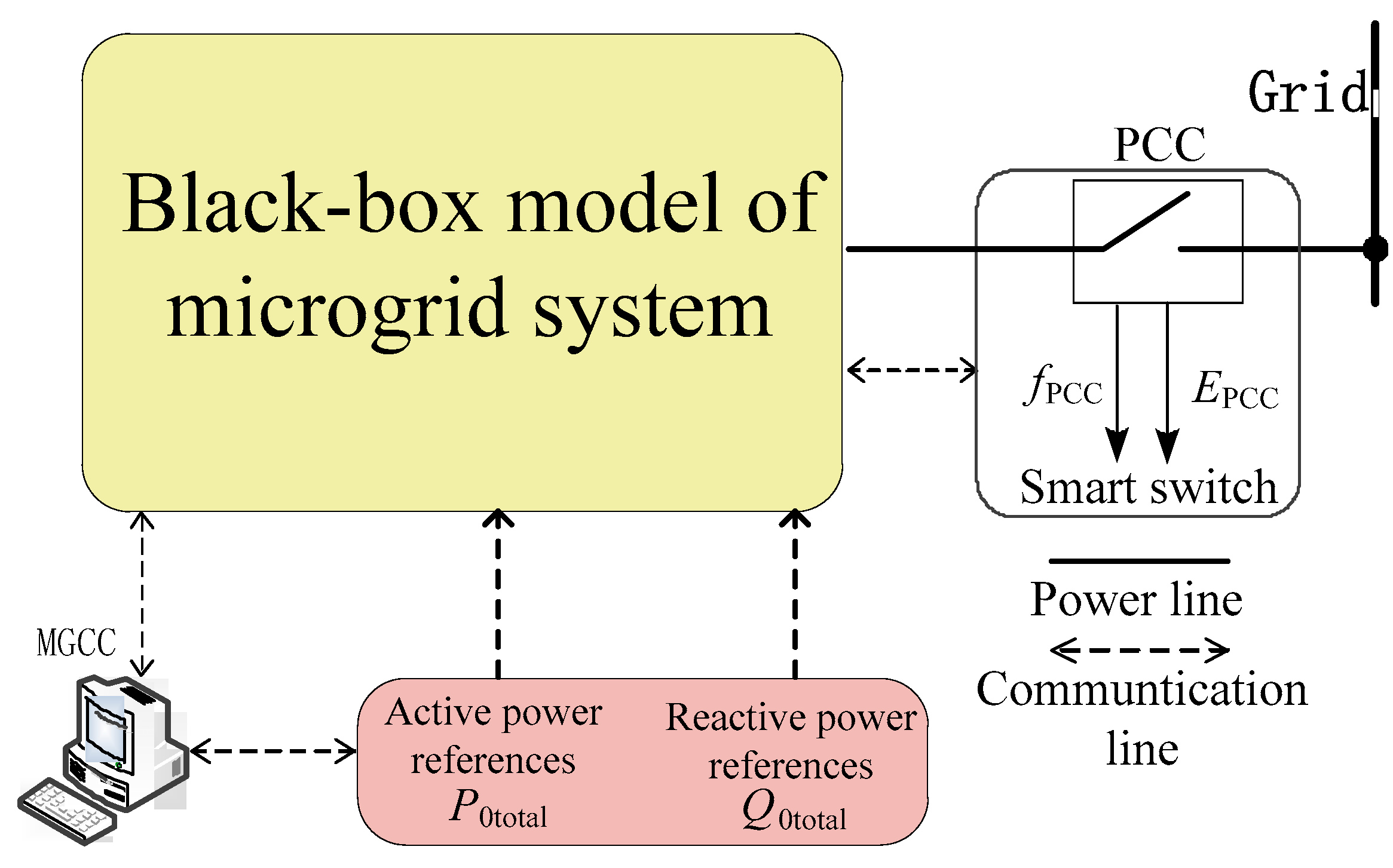
• The internal structure of the microgrid system and the types of loads are not considered at all. The method only pays attention to the response characteristics observed at PCC to ensure that the model structure is simple and easy to be applied.
• The proposed method is not confined to the analysis of relationship between power references and the voltage frequency, it is a general idea that can be applied in analyzing other port data of microgrid.
• Meanwhile, this method is also applicable to all kinds of microgrid systems, such as AC microgrids, DC microgrids, AC/DC hybrid microgrids, and microgrids with various types of electrical equipment and loads (like rotating generators based DG, inverter connected distributed energy resource (DER), controllable and uncontrollable loads, etc.).

2. Topology and Modeling Requirements of Microgrid

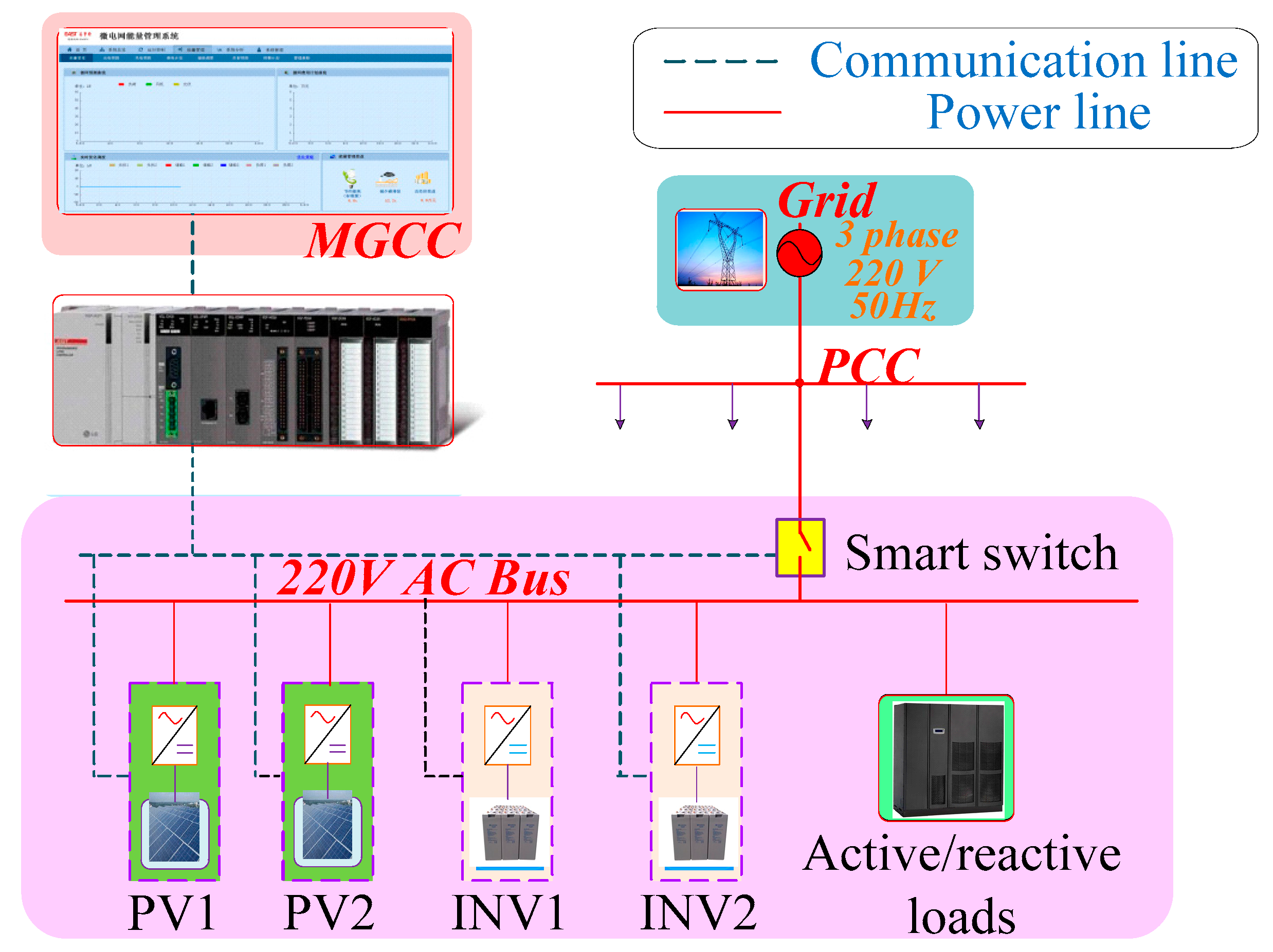
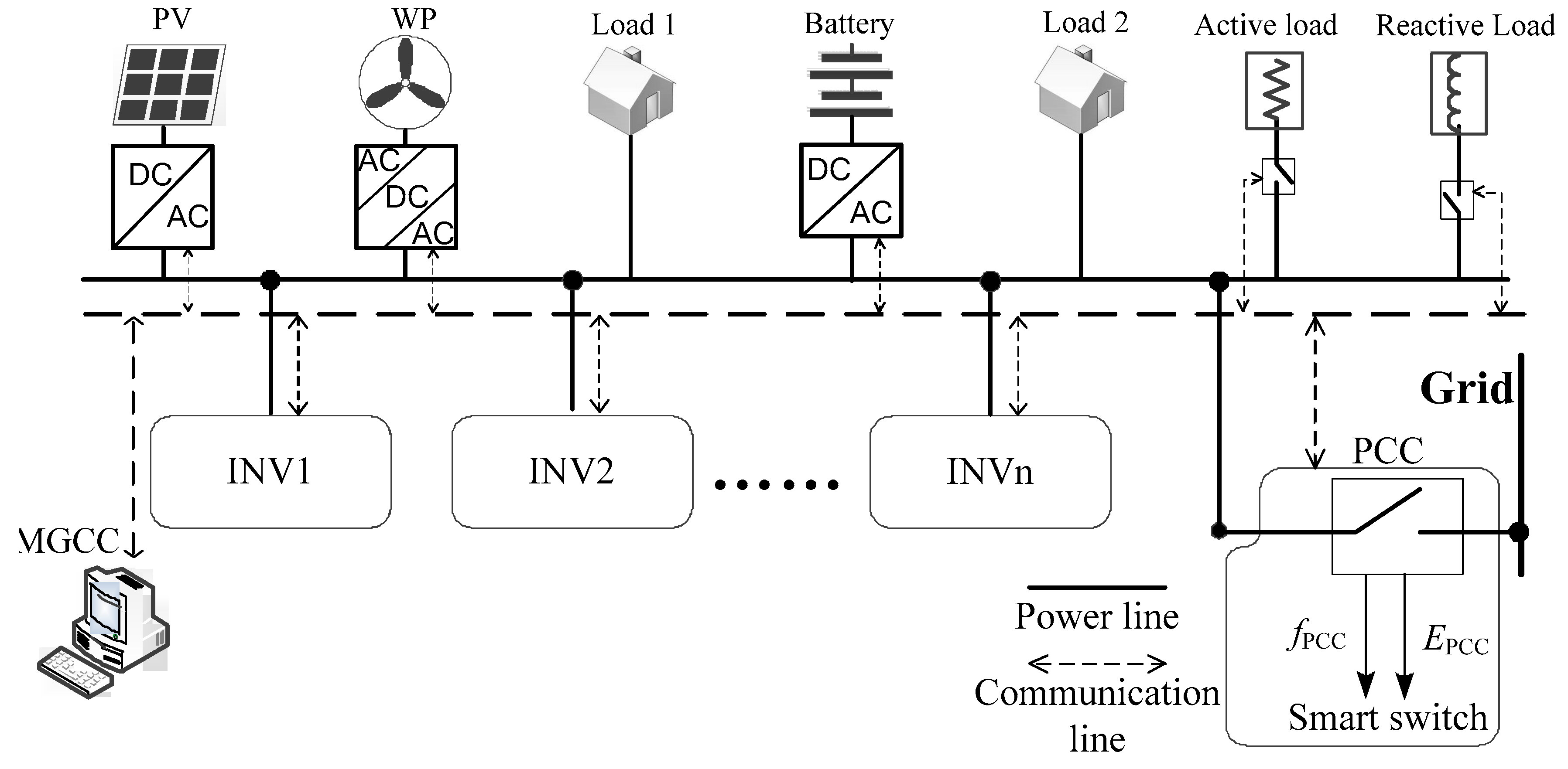
2.1. Typical Topology of Microgrid System

The typical microgrid topology is shown in Figure 1. The system commonly comprises DGs such as photovoltaic and wind power generations, as well as large-capacity energy storage devices that maintain the stability of the microgrid voltage and frequency. These devices are connected to the AC bus via the inverters. Some active and reactive loads are also included in the microgrid system. Equipment with communication functions such as specific DGs and smart switches can be connected to the microgrid central controller (MGCC) which can also send control instructions to DGs and smart switches in turn. When the smart switch at PCC is disconnected, the whole microgrid system operates in islanded mode. At this time, the microgrid can adopt a peer-to-peer control structure, and then use the control strategy such as droop control [19] and virtual synchronous machine control [20] to form the voltage and frequency of the microgrid.

2.2. Modeling Requirements

When studying the coordinated control of the microgrid system, usually the first step is to model and analyze the DGs included in the microgrid system, which is an important part before the overall modeling of microgrid. A rule of thumb is to use the mechanism modeling method to equivalent multiple energy storage inverters of the same type into one inverter so that the microgrid model can be greatly simplified. However, in most microgrid systems, besides the energy storage devices, there are various types of distributed power devices, which affect the system characteristics as well. These factors cannot be ignored, which lead to the model being too complex. Without the information of the internal structure of the microgrid system, the microgrid model can be equivalent to a black-box model and identification modeling method can be adopted to model the microgrid system.

According to the black-box model of microgrid as shown in Figure 2, the parameters optimization of secondary voltage and frequency controller can be carried out with less complexity. The black-box model of microgrid is considered as part of the open-loop transfer function of the overall control structure, and the corresponding root locus can be obtained according to the open-loop transfer function. Hence, the performance of microgrid system can be analyzed and the parameters of PI regulators can be optimized as well.

3. Identification of Black-Box Model

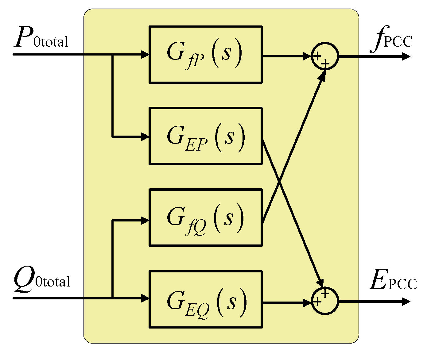
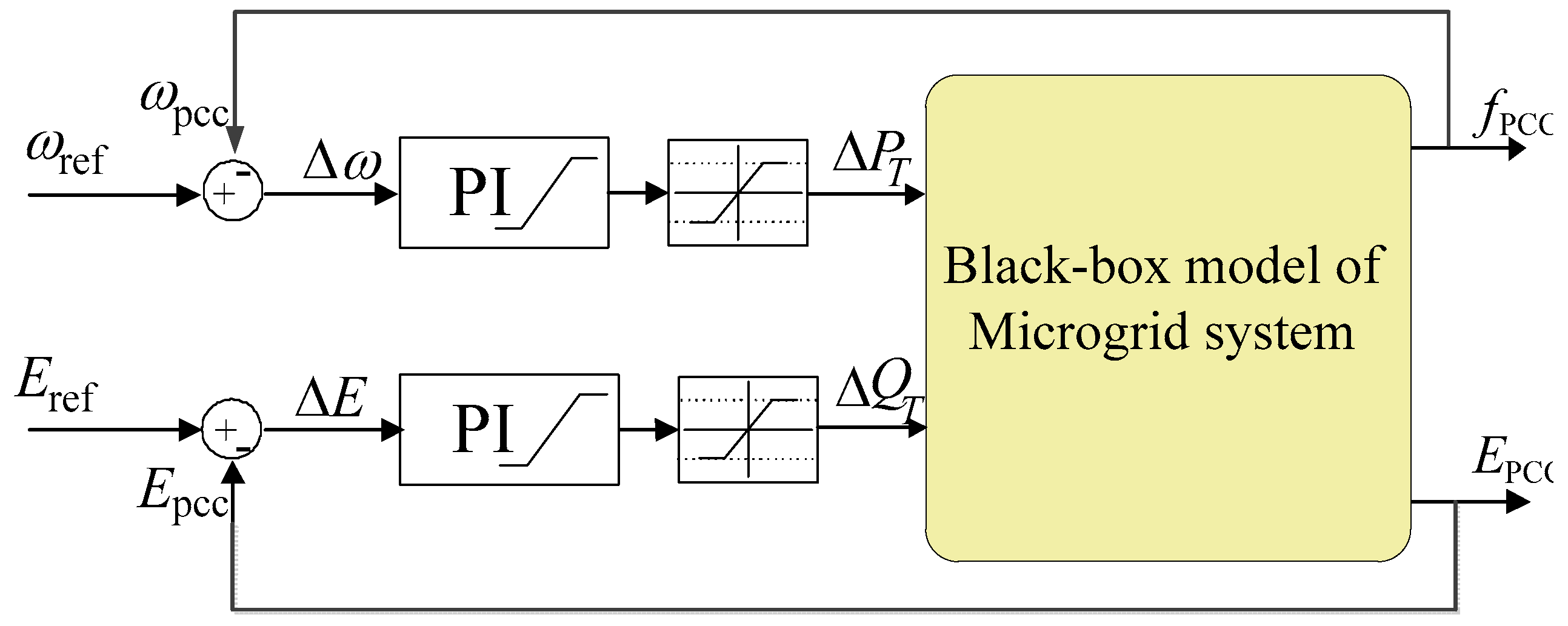
3.1. The Structure of Identification Model

According to the modeling requirements discussed above, the equivalent structure of microgrid model can be obtained as shown in Figure 3. Instead of analyzing the internal structure of the microgrid, the black-box model can be directly constructed by sampling the active and reactive power references data at the input ports and the frequency and voltage amplitude data at the output ports.

In theory, if the line impedance and the output impedance of the inverters included in the microgrid system are purely inductive, the relationship between the frequency and the active power, as well as the relationship between the voltage and the reactive power are completely decoupled. However, in practical microgrid systems, the line impedance and the output impedance are not purely inductive, so the coupling term should be considered in the black-box model. Therefore, there are 4 parameters to be identified in the black-box model as shown in Equation (1):

$$\left(\begin{array}{c}{f}_{\mathrm{PCC}}\\ E_{\mathrm{PCC}}\end{array}\right)=\left(\begin{array}{cc}{G}_{fP}(s)& G_{fQ}(s)\\ G_{EP}(s)& G_{EQ}(s)\end{array}\right)\left(\begin{array}{c}{P}_{0\mathrm{total}}\\ Q_{0\mathrm{total}}\end{array}\right)$$

(1)

where P_0total and Q_0total refer to the total active and reactive power references in the microgrid respectively, and according to the power droop coefficients of each DG, MGCC assigns the total power reference values P_0total and Q_0total to each DG according to Equation (2):

$$\{\begin{array}{c}{m}_1{P}_1=m_2{P}_2=m_3{P}_3=\cdots =m_i{P}_i\\ n_1{Q}_1=n_2{Q}_2=n_3{Q}_3=\cdots =n_i{Q}_i\\ P_{0\mathrm{total}}=P_1+P_2+P_3+\cdots P_i\\ Q_{0\mathrm{total}}=Q_1+Q_2+Q_3+\cdots Q_i\end{array}$$

(2)

where m_i and n_i refer to the active and reactive power droop coefficients of ith inverter, P_i and Q_i refer to the active and reactive power references of ith inverter, and f_PCC and E_PCC are frequency and voltage amplitudes of PCC. G_fP(s) and G_EP(s) are transfer functions of the active power reference with respect to the frequency and the voltage amplitude of PCC respectively, G_fQ(s) and G_EQ(s) are the transfer functions of the reactive power reference with respect to the frequency and the voltage amplitude of PCC respectively. Among them, G_EP(s) and G_fQ(s) are added to the model specifically in order to analyze the cross-coupling effect.

According to Equation (1), the microgrid system is regarded as a two-input and two-output black-box model. Without involving the characteristics of a single DG, the black-box identification model of the whole microgrid system can be obtained as shown in Figure 4.

By changing the total active and reactive power references issued by MGCC and sampling the voltage and frequency response data from the smart switch, the voltage and frequency response model of microgrid can be constructed by on-line identification method.

3.2. Identification Experiments Design

Since the step experiment process is easy to realize and has good identification performance, the step response experiment is adopted to identify the transfer function of the model. In order to simplify the identification process of the transfer functions mentioned above, this work divides modeled transfer functions into two groups. As shown in Figure 5, one group carries out the step experiment by performing a step on the active power reference value, the other group carries out the step experiment by performing a step on the reactive power reference value.

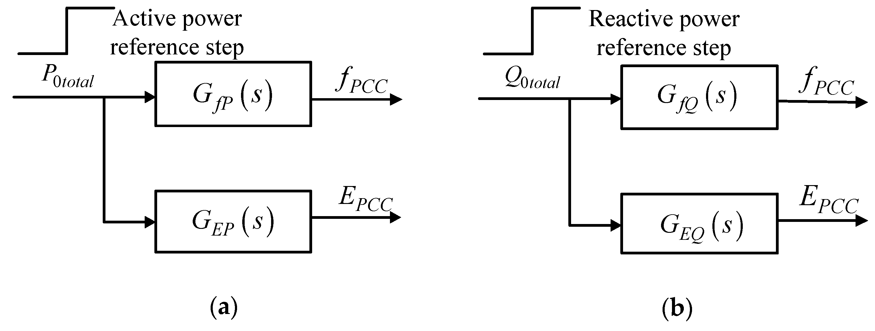
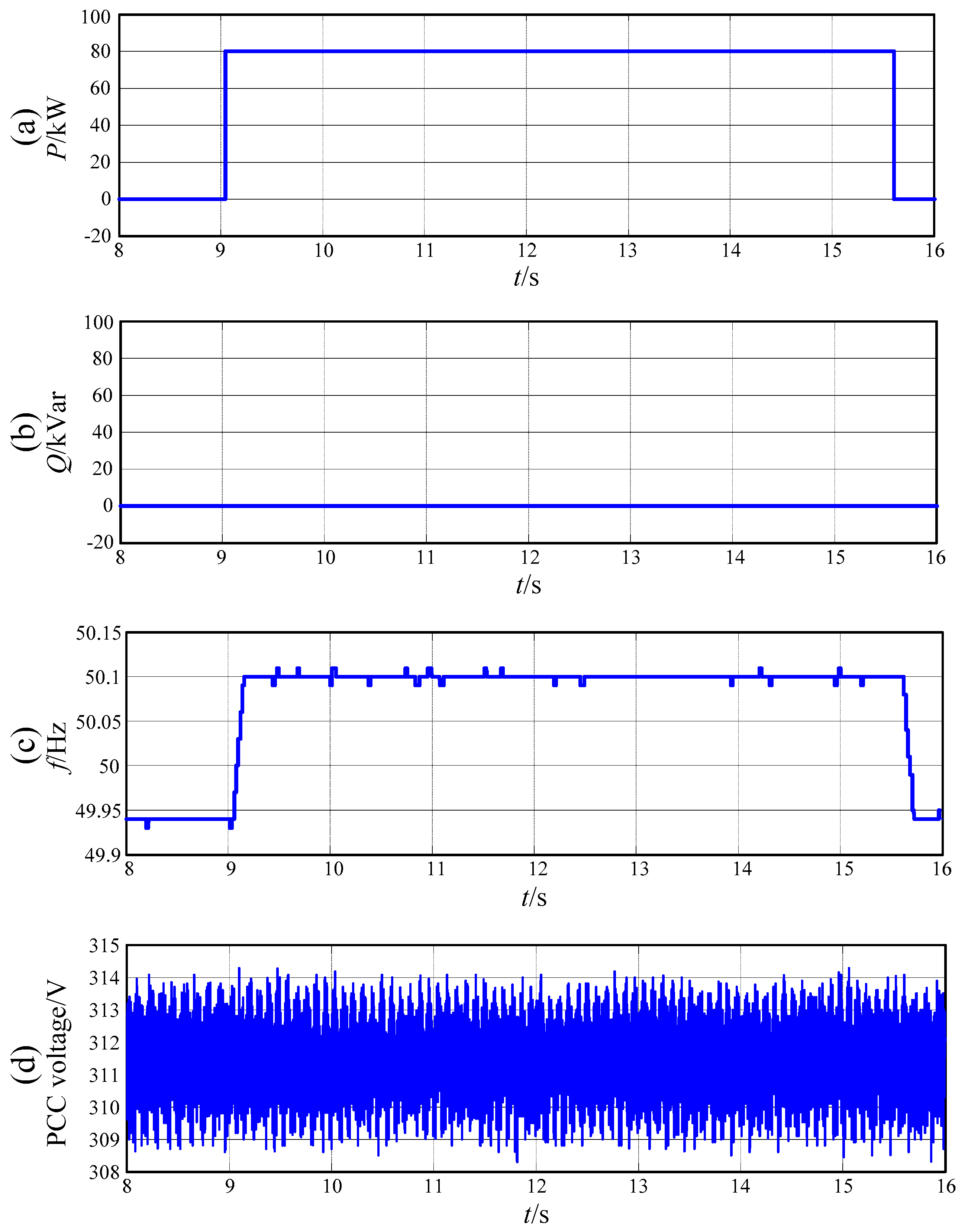
3.2.1. Active Power Reference Step

The active power reference step experiment is applied to identify G_fP(s) and G_EP(s). The Q_0total is set to 0, while the total active power reference is regarded as the input of the step experiment by performing a step on P_0total. At the same time, the f_PCC1 and E_PCC1 are sampled at PCC as the output of the step experiment.

$$\begin{array}{l}{G}_{fP}\left(s\right)=\frac{f_{\mathrm{PCC}}}{P_{0\mathrm{total}}}|{}_{Q_{0\mathrm{total}}=0}\\ G_{EP}\left(s\right)=\frac{E_{\mathrm{PCC}}}{P_{0\mathrm{total}}}|{}_{Q_{0\mathrm{total}}=0}\end{array}$$

(3)

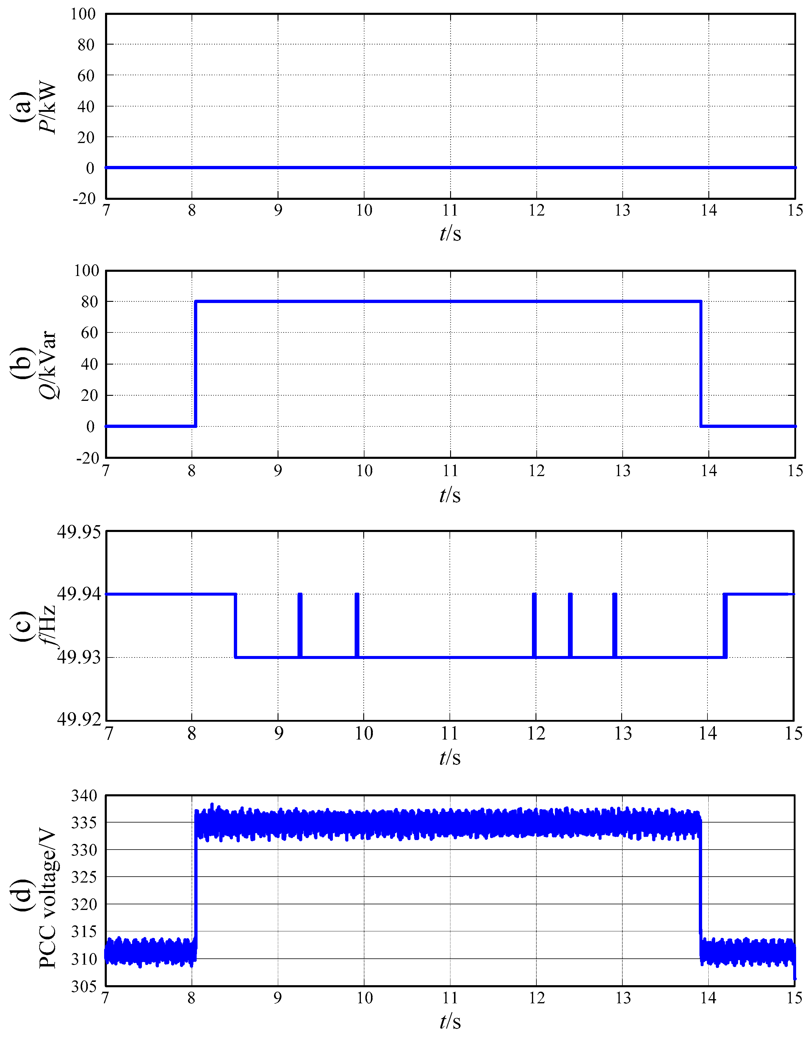
3.2.2. Reactive Power Reference Step

The reactive power reference step experiment is applied to identify G_fQ(s) and G_EQ(s). The P_0total is set to 0, while the total reactive power reference is regarded as the input of the step experiment by performing a step on Q_0total. Meanwhile, the f_PCC2 and E_PCC2 are sampled at PCC as the output of the step experiment.

$$\begin{array}{l}{G}_{fQ}\left(s\right)=\frac{f_{\mathrm{PCC}}}{Q_{0\mathrm{total}}}|{}_{P_{0\mathrm{total}}=0}\\ G_{EQ}\left(s\right)=\frac{E_{\mathrm{PCC}}}{Q_{0\mathrm{total}}}|{}_{P_{0\mathrm{total}}=0}\end{array}$$

(4)

3.3. Identification Strategy and Process

By sampling the input and output data of the microgrid system, the transfer function expressions of the microgrid model shown in Figure 4 can be obtained through an identification algorithm. The existing identification algorithms usually use the recursive least squares method to identify the system on-line and keep updating the parameters in real time. However, as the covariance matrix decreases in the recursive process, the parameters are prone to explode [21]. In order to enhance the stability of the recursive process, a damping term can be added to suppress the parameter explosion. Therefore, the recursive damped least squares method is used in this paper as the identification algorithm.

Moreover, in the classical control method for discrete systems, the bilinear transformation can ensure that the continuous system and the discrete system have the same stability and the same steady-state gain [22]. Therefore, the bilinear transformation is chosen to discretize the transfer functions shown in Equations (2) and (3), and the recursive damped least squares method is used for the parameter identification.

This paper takes G_fP(s) as an example and analyzes the identification process in detail, other transfer functions G_EP(s), G_fQ(s) and G_EQ(s) can adopt the same process.

3.3.1. Data Preprocessing

The first task is to preprocess the sampled data P_0total and E_PCC1. It mainly includes two steps:

• Offset removal: The black-box model of the microgrid system includes the steady-state component and the dynamic component. But the parameters to be identified only involve the system dynamics of the system model, thus it is necessary to remove the steady-state components, i.e., the steady-state values of the input and output signals (before the step is done) respectively.
• Measurement prefiltering: Since the sampling data contains some ripple and noise caused by the switching frequency, prefiltering input and output data should be considered before the recursive process to avoid the identification accuracy being affected.

3.3.2. Model Order and Initial Value Selection

Secondly, the number of coefficients of each polynomial (transfer function order) and the initial values of parameters should be determined. The first n data to be identified (in order to reduce the computation load, the selected data should not be too much) can be selected, and the least squares algorithm can be used to test a certain transfer function order iteratively. By comparing the fitness between the model output and the measured output in different orders, the order of the transfer function G_fP(s) can be determined and remains constant in the process of recursion. The fitting performance can be calculated as follows:

$$f_{\mathrm{Best} \mathrm{fit}}=100\%\times \left(1-\frac{\sqrt{{\displaystyle \sum _{k=1}^N{(y(k)-\overline{y})}^2}}}{\sqrt{{\displaystyle \sum _{k=1}^N{(y(k)-\widehat{y}(k))}^2}}}\right)\overline{y}=\frac{1}{N}{\displaystyle \sum _{K=1}^{N}y(k)}$$

(5)

where y(k) is the measured output of microgrid, $\widehat{y}$(k) is the model output, $\overline{y}$ is the average value of the measured output. The higher the f_{Best fit}, the better the model can reproduce the output characteristics of the microgrid port. Considering that the high model order affects the computing speed significantly, so as long as the fitness meets the requirements, choosing a lower transfer function order is recommended. Then, the order of the numerator of G_fP(s) is set to 1, while that of the denominator is 2, the corresponding expression of G_fP(s) can be obtained as

$$G_{f\mathrm{P}}(s)=\frac{f_{\mathrm{PCC}}(s)}{P_{0\mathrm{total}}(s)}=\frac{b_{1}s+b_2}{s^2+a_{1}s+a_2}$$

(6)

The transfer function can be discretized by the bilinear transformation, as shown in Equation (7):

$$G_{fP}=G_{fP}(s)|{}_{(s=\frac{Tz-1}{2z+1})}=\frac{B_1+B_2{z}^{-1}+B_3{z}^{-2}}{1+A_1{z}^{-1}+A_2{z}^{-2}}$$

(7)

where

$$\{\begin{array}{l}{A}_1=\left(-T^2/2+2a_2-a_{1}T\right)/\Delta \hfill \\ A_2=\left(T^2/4+a_{1}T/2+a_2\right)/\Delta \hfill \\ B_1=\left(b_2+b_{1}T/2\right)/\Delta \hfill \\ B_2=(2b_2-b_{1}T)/\Delta \hfill \\ B_3=(b_2+b_{1}T/2)/\Delta \hfill \\ \Delta =T^2/4+a_{1}T/2\hfill \end{array}$$

(8)

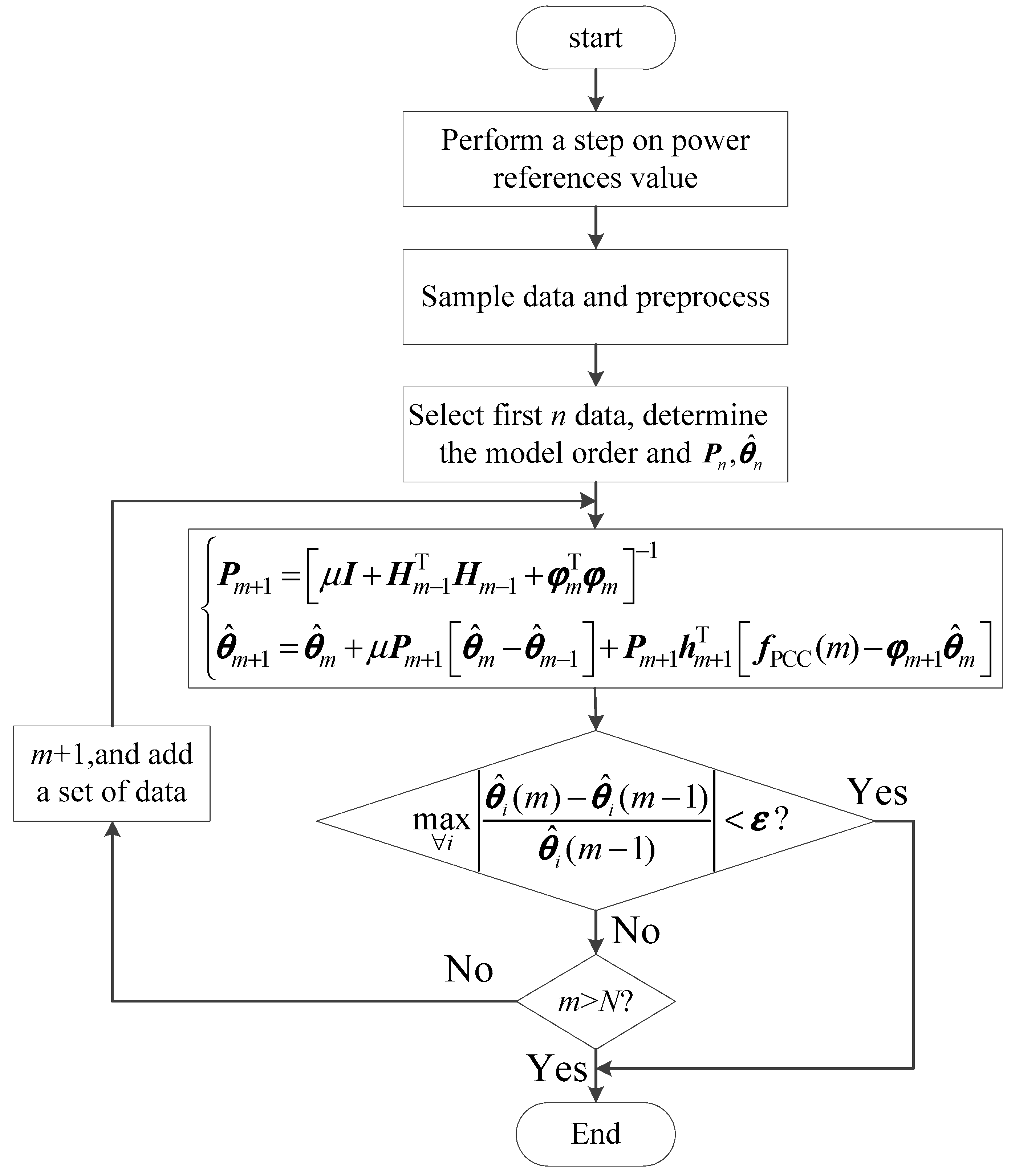
3.3.3. Online Recursive Algorithm

Then the corresponding difference equation of Equation (7) is:

$$f_{\mathrm{PCC}}(k)=-A_1{f}_{\mathrm{PCC}}(k-1)-A_2{f}_{\mathrm{PCC}}(k-2)+B_1{P}_{0\mathrm{total}}(k)+B_2{P}_{0\mathrm{total}}(k-1)+B_3{P}_{0\mathrm{total}}(k-2)$$

(9)

where f_PCC (k) and P_0total (k) are discrete values of f_PCC and P_0total at time k.

Let k = 3, 4,..., m, m is the total number of samples during the time of recursive computation. Equation (9) can be rewritten in the form of a matrix:

$${\mathit{F}}_m={\mathit{H}}_m\mathit{\theta }$$

(10)

where ${\mathit{F}}_m={\left[f_{PCC}(3),f_{PCC}(4),\cdots ,f_{PCC}(m)\right]}^{\mathrm{T}}$, ${\mathit{H}}_m={\left[{\phi }_3,{\phi }_4,\cdots ,{\phi }_m\right]}^{\mathrm{T}}$, $\theta ={\left[A_1,A_2,B_1,B_2,B_3\right]}^{\mathrm{T}}$, ${\mathit{\phi }}_m=\left[f_{\mathrm{PCC}}(m-1),f_{\mathrm{PCC}}(m-2),P_{\mathrm{total}}(m),P_{\mathrm{total}}(m-1),P_{total}(m-2)\right]$.

The idea of the recursive damped least squares method is to revise the estimated value $\stackrel{⌢}{\mathit{\theta }}$ recursively so that the minimum sum of squared errors between ${\mathit{F}}_m$ and ${\stackrel{⌢}{\mathit{F}}}_m={\mathit{H}}_m{\stackrel{⌢}{\mathit{\theta }}}_m$ can be obtained:

$$J(\stackrel{⌢}{\theta })={({\mathit{F}}_m-{\mathit{H}}_m{\stackrel{⌢}{\mathit{\theta }}}_m)}^{\mathrm{T}}({\mathit{F}}_m-{\mathit{H}}_m{\stackrel{⌢}{\mathit{\theta }}}_m)=\min$$

(11)

where $J(\stackrel{⌢}{\theta })$ is the objective function. As discussed above, adding damping to the algorithm can suppress parameter explosion, so a damping term is added on the basis of equation (11):

$$J(\stackrel{⌢}{\theta })={({\mathit{F}}_m-{\mathit{H}}_m{\stackrel{⌢}{\mathit{\theta }}}_m)}^{\mathrm{T}}({\mathit{F}}_m-{\mathit{H}}_m{\stackrel{⌢}{\mathit{\theta }}}_m)+\mu {\left[{\stackrel{⌢}{\mathit{\theta }}}_m-{\stackrel{⌢}{\mathit{\theta }}}_{m-1}\right]}^{\mathrm{T}}{\left[{\stackrel{⌢}{\mathit{\theta }}}_m-{\stackrel{⌢}{\mathit{\theta }}}_{m-1}\right]}^{\mathrm{T}}$$

(12)

where $\mu$ is the damping factor, which is related to the linearity of the identification model.

This paper adopts the adaptive damping factor method to adjust the value of $\mu$. Firstly, the matrix ${\mathit{H}}_n{\mathit{H}}_n^T$ is employed to determine the initial value of $\mu$:

$${\mu }_0=0.01\times \mathrm{mean}({\mathit{H}}_n{\mathit{H}}_n^T)$$

(13)

where the function mean is to compute the average value of the matrix. The linearity of the microgrid black-box model can be quantitatively evaluated by the ratio of the reduction and the change of the objective function J in the iterative process [22]:

$$\lambda =\frac{J({\stackrel{⌢}{\theta }}_m)-J({\stackrel{⌢}{\theta }}_{m-1})}{\tilde{J}({\stackrel{⌢}{\theta }}_m)-J({\stackrel{⌢}{\theta }}_{m-1})}$$

(14)

where $J({\stackrel{⌢}{\theta }}_m)$ is the calculated value of the objective function J at time m, $\tilde{J}({\stackrel{⌢}{\theta }}_m)$ is the second-order Taylor series expansion of the objective function J at time m:

$$\tilde{J}({\stackrel{⌢}{\theta }}_m)=J({\stackrel{⌢}{\theta }}_n)+J^{\prime }({\stackrel{⌢}{\theta }}_n)({\stackrel{⌢}{\theta }}_m-{\stackrel{⌢}{\theta }}_n)+\frac{J^{″}({\stackrel{⌢}{\theta }}_n)}{2}{({\stackrel{⌢}{\theta }}_m-{\stackrel{⌢}{\theta }}_n)}^2$$

(15)

where $J^{\prime }$ is the first derivative of $J$, $J^{″}$ is the second derivative of $J$.

Therefore, the damping factor can be corrected using the value calculated in Equation (14):

• Under the condition of $\lambda$ < 0.3, it shows that the objective function J exhibits a linearity reduction trend during the recursive process, $\mu$ is needed to increase in the subsequent recursive process to ensure better frequency and voltage identification
• Under the condition of 0.3 < $\lambda$ < 0.7, it indicates that the objective function $J$ has a small change in linearity during the recursive process, therefore the damping factor is close to the best value and there is no need to change it.
• Under the condition of $\lambda$ > 0.7, a smaller damping factor $\mu$ should be chosen.

In order to achieve the adaptive correction of damping factor during the identification process, Proportional coefficient $\eta$ is employed, whose value is generally between 2 and 10, as shown below:

$$\eta =\frac{J({\stackrel{⌢}{\theta }}_m)-J({\stackrel{⌢}{\theta }}_{m-1})}{(f_{\mathrm{PCC}}(m)-\phi (m)\cdot x_k)\cdot x_k}+2$$

(16)

when $\mu$ is needed to be increased, $\mu$ can be taken as

$$\mu ={\mu }_0\cdot \eta$$

(17)

on the contrary, when $\mu$ is needed to be decreased, $\mu$ can be taken as

$$\mu ={\mu }_0/\eta$$

(18)

According to the extremum principle, the minimum value of J can be obtained by taking the differentiation to the right part of Equation (12). Through combing Equations (10)–(12), the recursive equation based on recursive damped least square method is derived as below:

$$\{\begin{array}{l}{\mathit{P}}_{m+1}={\left[\mu \mathit{I}+{\mathit{H}}_{m-1}^{\mathrm{T}}{\mathit{H}}_{m-1}+{\mathit{\phi }}_m^{\mathrm{T}}{\mathit{\phi }}_m\right]}^{-1}\hfill \\ {\widehat{\mathit{\theta }}}_{m+1}={\widehat{\mathit{\theta }}}_m+\mu {\mathit{P}}_{m+1}\left[{\widehat{\mathit{\theta }}}_m-{\widehat{\mathit{\theta }}}_{m-1}\right]+{\mathit{P}}_{m+1}{\mathit{h}}_{m+1}^{\mathrm{T}}\left[{\mathit{f}}_{\mathrm{PCC}}(m)-{\mathit{\phi }}_{m+1}{\widehat{\mathit{\theta }}}_m\right]\hfill \end{array}$$

(19)

Ever since a set of observation data $\phi$_m is added, P_m and $\widehat{\theta }$_m are revised once, therefore new estimation values of parameters are derived and on-line identification of parameters are realized. The identification procedure is shown in Figure 6. Where ε is the allowable range of precision error, N is the total number of samples at the current moment. When the recursive algorithm compute to the sampling moment or the parameters estimation does not change, the recursive process is terminated until the new sampling data arrives. After obtaining the parameters of the transfer function G_fP(z), the bilinear inverse transformation can be carried out to convert the transfer function from discrete domain to continuous domain.

4. Experiments and Model Validation

In this paper, a series of model identification experiments are carried out on a microgrid test platform to verify the accuracy of the proposed modeling method. The controllers of the two inverters integrated into the microgrid use MCU (TMS320F28335, Texas Instruments, Inc, Dallas, TX, USA), the pulse width modulation (PWM) carrier frequency of each controller is set to 6 kHz, and the integrated three-phase resistive load is configured to 30 kW. Both inverters operate in P-f droop control mode. Active and reactive power droop coefficients are chosen as 4 × 10⁻⁶ and 4 × 10⁻⁴ respectively. Under the normal operation of the experimental platform, the input and output data are sampled by the Yokogawa recorder. All devices are connected to the AC Bus and communication lines, the structure of the microgrid test platform is shown in Figure 7.

4.1. Identification Experiments of G_fP(s) and G_EP(s)

To carry out the identification experiments of G_fP(s) and G_EP(s), parallel inverters and the three-phase active load are integrated into the microgrid. After the system reaches a steady state, the active and reactive power references are set to 0 by MGCC at first. Then the active power reference is changed to 80 kW at 9 s, and set to 0 again at 15.7 s. During this experiment, the reactive power reference remains at 0. Figure 8 shows the identification data P_0total, E_PCC1, and f_PCC1 sampled by the waveform recorder at PCC.

According to the identification process shown in Figure 6, the sampled data P_0total and f_PCC1 can be used to identify the model transfer function G_fP(s).

$$G_{fP}(s)=\frac{4.229\cdot {10}^{-8}{s}^2-0.001s+5.0184}{s^2+945.97s+2.5172\cdot {10}^5}$$

(20)

By applying the same input on both the model and the microgrid system, the fitting performance can be obtained as shown in Figure 9. Since only the dynamic component is analyzed, the steady-state component contained in each measurement has to be removed. As it can be seen, the model output matches the microgrid output properly, and f_{Best fit} reaches 95.36.

Similarly, using the sampled data P_0total and E_PCC1, the transfer function G_EP(s) can be obtained:

$$G_{EP}(s)=\frac{0.06107s^2+64.24s+152.9}{s^3+1249s^2+3.95\cdot {10}^{5}s+4.933\cdot {10}^8}$$

(21)

4.2. Identification Experiments of G_fQ(s) and G_EQ(s)

To carry out the identification experiments of G_fQ(s) and G_EQ(s), parallel inverters and the three-phase reactive load are integrated into the microgrid. After the system reaches a steady state, the active and reactive power references are set to 0 by MGCC at first. Then the reactive power reference is changed to 80 kVar at 9 s, and set to 0 again after 5.6 s. During this experiment, the active power reference remains at 0. Figure 10 shows the identification data Q_0total, E_PCC2, and f_PCC2 sampled by the waveform recorder at PCC.

According to the identification process shown in Figure 6, the sampled data Q_0total and E_PCC2 can be used to identify the model transfer function G_EQ(s).

$$G_{EQ}(s)=\frac{1.0129\cdot {10}^{-5}{s}^2-1.288s+7826.65}{s^2+2760.77s+2.545\cdot {10}^6}$$

(22)

By applying the same excitation on both the model and the microgrid system, the fitting performance can be obtained as shown in Figure 11. Clearly, the model output also matches the microgrid output, and f_{Best fit} reaches 90.72.

Similarly, using the sampled data Q_0total and f_PCC2, the transfer function G_fQ(s) can be obtained as follows:

$$G_{fQ}(s)=\frac{8.085\cdot {10}^{-6}{s}^2+2.219\cdot {10}^{-4}s+6.091\cdot {10}^{-4}}{s^3+8.47s^2+710.6s+5187}$$

(23)

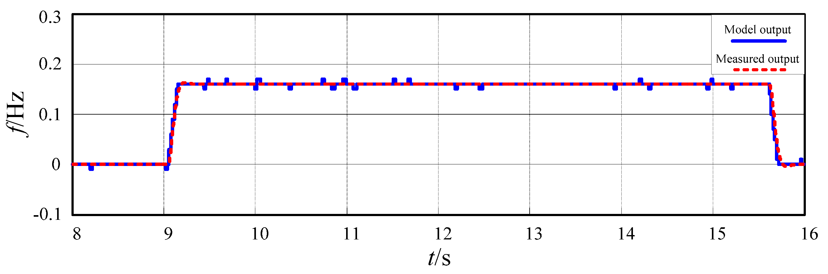
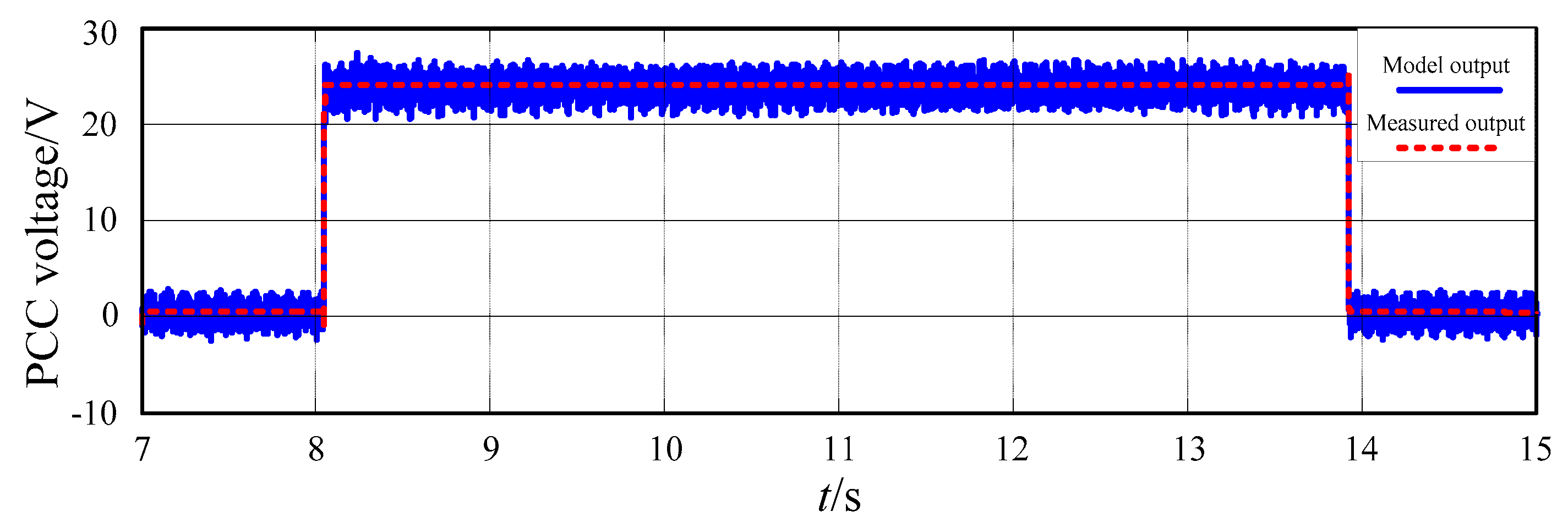
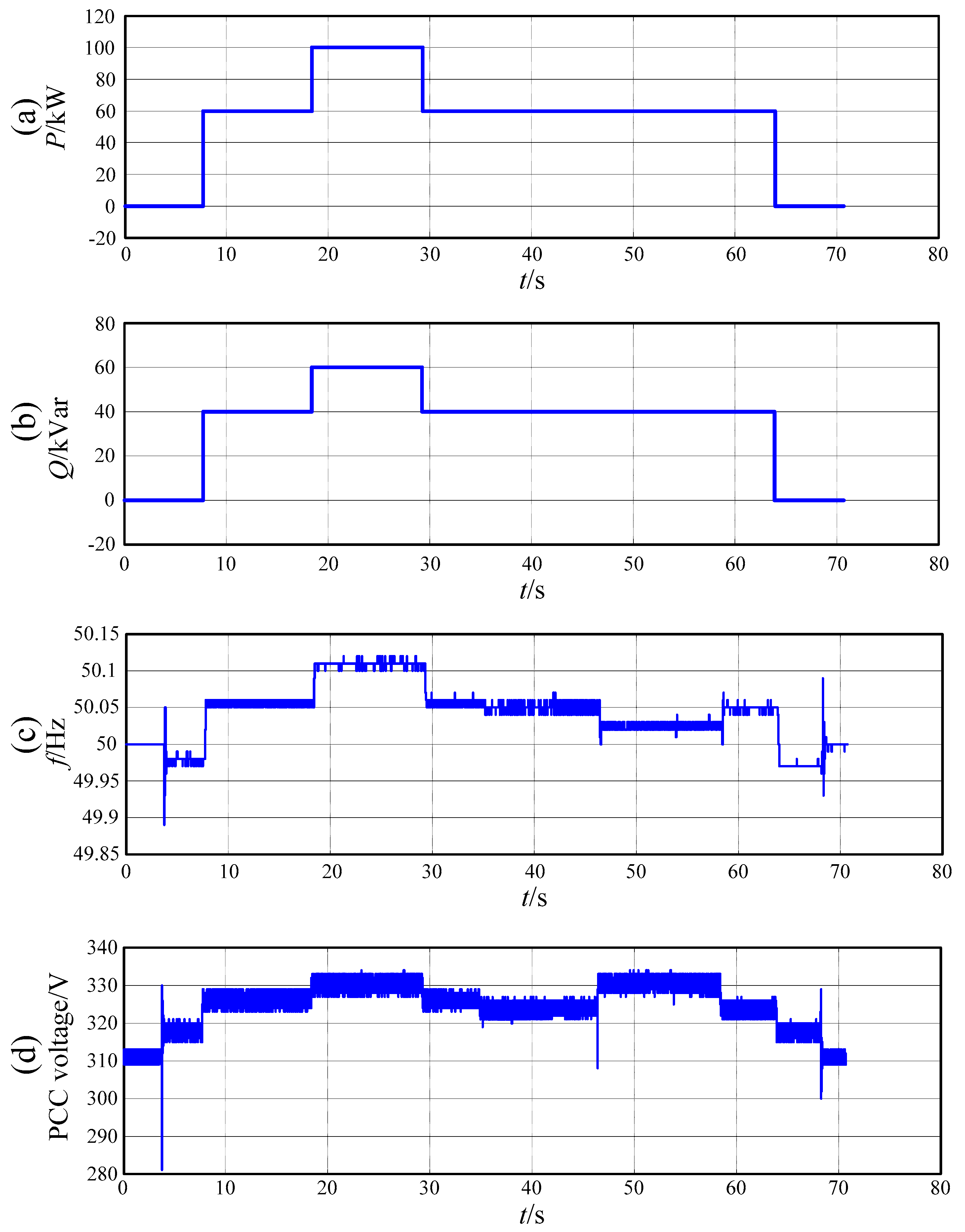
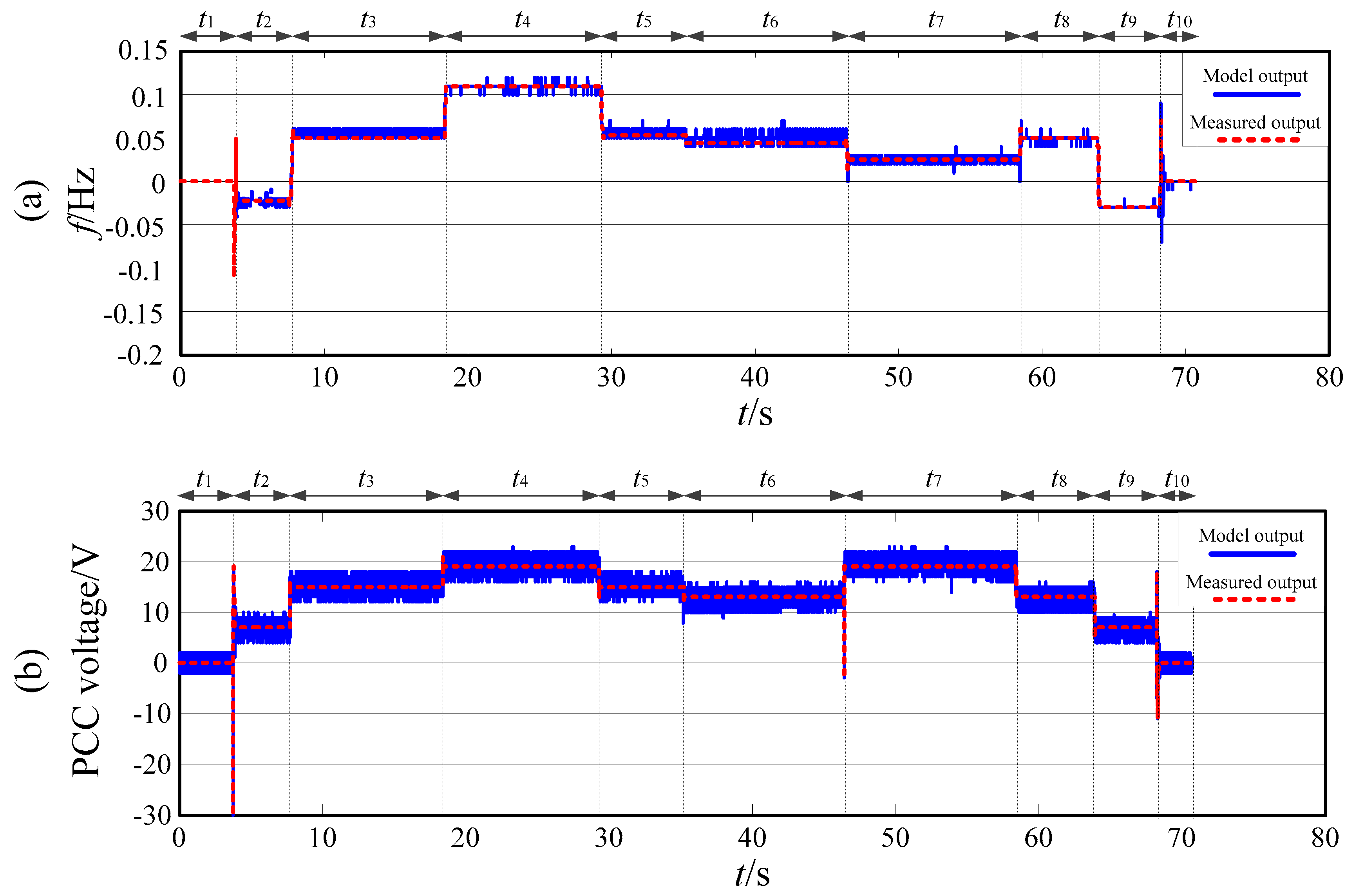
4.3. Recursive Model Validation

According to the power references step experiments, the voltage frequency response model is obtained under the certain microgrid structure. Furthermore, in order to verify the adaptability of the recursive damped least squares method applied in the model identification, that is, the online identification effect during the period of microgrid structure changing, several adjustments have been made: active power droop coefficients of two inverters are changed to 4 × 10⁻⁶ and 8 × 10⁻⁶ respectively; reactive power droop coefficients are changed to 2 × 10⁻⁴ and 4 × 10⁻⁴ respectively; the PV inverter which is supplied by Chroma solar PV array simulators is added to the microgrid structure, and the maximum output power of the PV inverter is set to 4 kW. During the power references step experiment, the number of inverters connected to the microgrid are changed, the active and reactive loads are set to different parameters, as listed in

Table 1. Experimental parameters.

Time	Total Power References	Active Load	Reactive Load
t1	0/0	0	0
t2	0/0	12 kW	20 kVar
t3	60 kW/40 kVar	12 kW	20 kVar
t4	100 kW/60 kVar	12 kW	20 kVar
t5	60 kW/40 kVar	12 kW	20 kVar
t6	60 kW/40 kVar	8 kW	10 kVar
t7	60 kW/40 kVar (INV1 shutdown)	8 kW	10 kVar
t8	60 kW/40 kVar (INV1 start up)	8 kW	10 kVar
t9	0/0	8 kW	10 kVar
t10	0/0	0	0

.

The input and output data during the experiment are recorded by the waveform recorder, as shown in Figure 12.

Meanwhile, the same experimental processes as shown in Table 1 are carried out on a corresponding simulation model under the MATLAB/Simulink environment (2014a, The MathWorks, Inc, Natick, MA, USA), which is constructed according to the black-box equivalent model shown in Figure 4. Initial values of P and $\widehat{\theta }$ can be figured out according to the transfer function parameters obtained in Section 3.2 and Section 4.1. The frequency and voltage output of the simulation model can be obtained by using the recursive damped least squares method for online identification.

The experimental and simulation results are compared with each other, as shown in Figure 13. It can be seen that the simulation model is able to reproduce the system responses of the microgrid system during the experiment, especially when the frequency and voltage responses of the microgrid have step changes, the output of the simulation model tracks the changes accurately. Hence, the identification algorithm implemented in the simulation model is validated.

5. Conclusions

In this paper, the black-box modeling technique of voltage frequency response model of microgrid system has been studied. In terms of the parameter identification algorithm of the recursive damped least squares, the model can be identified and is suitable for performing simulations of microgrid system on system level, especially when the internal information of a microgrid cannot be accessed. The procedure of constructing the black-box model of microgrid is analyzed emphatically. Compared with the traditional method of mechanism modeling, this method greatly simplifies the modeling steps and provides a general idea for microgrid system modeling.

The output data obtained from the simulation model has been compared with the measured output under the conditions of changing the microgrid structure. Depending on the recursive algorithm, the identification model can reproduce the frequency and voltage characteristics of the microgrid port accurately in all cases, which indicates that the black-box identification modeling method has a wide range of adaptability to realize on-line identification of the microgrid system.

In future, in order to improve the identification accuracy, the influence of different communication delays on the proposed identification strategy needs to be further studied. In addition to this, how to apply the proposed identification model to a secondary frequency and voltage regulation control system, so as to optimize parameters of secondary voltage and frequency controllers, are also set as the future research directions.

References

1. Yu, X.D.; Xu, X.D.; Chen, S.Y.; Wu, J.Z.; Jia, H.J. A brief review to integrated energy system and energy internet. Trans. Chin. Electrotech. Soc. 2016, 31, 1–13. [Google Scholar]
2. Hou, X.B.; Wang, L.; Li, Q.M.; Wang, J.; Liu, J.Z.; Qian, X.S. Review of key technologies for high-voltage and high-power transmission in space solar power station. Trans. China Electrotech. Soc. 2017, 15, 61–73. [Google Scholar]
3. Zheng, W. Identification Modeling Method and Application of Photovoltaic Grid-Connected Inverter. Ph.D. Thesis, Chongqing University, Chongqing, China, 2014. [Google Scholar]
4. Wang, X.; Blaabjerg, F.; Chen, Z. Autonomous control of inverter interfaced DG units for harmonic current filtering and resonance damping in an islanded microgrid. IEEE Trans. Ind. Appl. 2014, 50, 452–461. [Google Scholar] [CrossRef]
5. Jadhav, G.N.; Changan, D.D. Modeling of inverter for stability analysis of microgrid. In Proceedings of the IEEE 7th Power India International Conference (PIICON), Bikaner, India, 25–27 November 2016; pp. 1–6. [Google Scholar]
6. Xiong, X.F.; Chen, K.; Zheng, W.; Shen, Z.J.; Shahzad, N.M. Photovoltaic inverter model identification based on least squares method. Power Syst. Prot. Control 2012, 22, 52–57. [Google Scholar]
7. Jin, Y.Q.; Ju, P.; Pan, X.P. A stepwise method to identify controller parameters of photovoltaic inverter. Power Syst. Technol. 2015, 39, 594–600. [Google Scholar]
8. Zheng, W.; Xiong, X.F. A model identification method for photovoltaic grid-connected inverters based on the Wiener model. Proc. CSEE 2013, 33, 18–26. [Google Scholar]
9. Zheng, W.; Xiong, X.F. System identification for NARX model of photovoltaic grid-connected inverter. Power Syst. Technol. 2013, 39, 2440–2445. [Google Scholar]
10. Valdivia, V.; Barrado, A.; Lázaro, A.; Sanz, M.; del Moral, D.L.; Raga, C. Black-Box behavioral modeling and identification of DC–DC converters with input current control for fuel cell power conditioning. IEEE Trans. Ind. Electron. 2014, 61, 1891–1903. [Google Scholar] [CrossRef]
11. Frances, A.; Asensi, R.; Garcia, O.; Prieto, R.; Uceda, J. How to model a DC microgrid: towards an automated solution. In Proceedings of the IEEE Second International Conference on DC Microgrids (ICDCM), Nuremburg, Germany, 27–29 June 2017. [Google Scholar]
12. Valdivia, V.; Lazaro, A.; Barrado, A.; Zumel, P.; Fernandez, C.; Sanz, M. Black-box modeling of three-phase voltage source inverters for system-level analysis. IEEE Trans. Ind. Electron. 2012, 59, 3648–3662. [Google Scholar] [CrossRef]
13. Valdivia, V.; Todd, R.; Bryan, F.J.; Barrado, A.; Lázaro, A.; Forsyth, A.J. Behavioral modeling of a switched reluctance generator for aircraft power systems. IEEE Trans. Ind. Electron. 2014, 61, 2690–2699. [Google Scholar] [CrossRef]
14. Francés, R.; Asensi, R.; García, O.; Prieto, R.; Uceda, J. The performance of polytopic models in smart DC microgrids. In Proceedings of the IEEE Energy Conversion Congress and Exposition (ECCE), Milwaukee, WI, USA, 18–22 September 2016; pp. 1–8. [Google Scholar]
15. Erlinghagen, P.; Wippenbeck, T.; Schnettler, A. Modelling and sensitivity analyses of equivalent models of low voltage distribution grids with high penetration of DG. In Proceedings of the 50th International Universities Power Engineering Conference (UPEC), Stoke on Trent, UK, 1–4 September 2015; pp. 1–5. [Google Scholar]
16. Francés, A.; Asensi, R.; García, O.; Uceda, J. A blackbox large signal Lyapunov-based stability analysis method for power converter-based systems. In Proceedings of the IEEE 17th Workshop on Control and Modeling for Power Electronics (COMPEL), Trondheim, Norway, 27–30 June 2016; pp. 1–6. [Google Scholar]
17. Cao, P.P.; Zhang, X.; Yang, S.Y.; Xie, Z.; Guo, L.L. Online rotor time constant identification of induction motors based on Lyapunov stability theory. Proc. CSEE 2016, 36, 3947–3955. [Google Scholar]
18. Yang, S.Y.; Sun, R.; Cao, P.P.; Zhang, X. Double compound manifold sliding mode observer based rotor resistance online updating scheme for induction motor. Trans. Chin. Electrotech. Soc. 2018, 33, 3596–3606. [Google Scholar]
19. Chen, J.; Liu, M.A.; Chen, X.; Niu, B.W.; Gong, C.Y. Wireless parallel and circulation current reduction of droop-controlled inverters. Trans. Chin. Electrotech. Soc. 2018, 33, 1450–1460. [Google Scholar]
20. Tu, C.M.; Yang, Y.; Lan, Z.; Xiao, F.; Li, Y.T. Secondary frequency regulation strategy in microgrid based on VSG. Trans. Chin. Electrotech. Soc. 2018, 33, 2186–2195. [Google Scholar]
21. Zhao, X.; Wang, Z.P.; Jia, H.H. Comparison and analysis of discretization methods for continuous systems. Ind. Inf. Technol. Educ. 2015, 12, 71–76. [Google Scholar]
22. Su, Y.C. The Research of Leven-Marquadt-Fletcher Method for Fitting Transient Electromagnetic Data. Ph.D. Thesis, Jilin University, Shenyang, China, 2009. [Google Scholar]
Figure 1. Topological Structure of Microgrid System.
Energies 12 02049 g001
Figure 2. Microgrid Black-Box Model for Secondary Frequency and Voltage Regulation Control Structure.
Energies 12 02049 g002
Figure 3. Black-box model structure of microgrid.
Energies 12 02049 g003
Figure 4. Equivalent black-box model of voltage frequency response of microgrid.
Energies 12 02049 g004
Figure 5. Input power references step experiments (a) Active power references step; (b) Reactive power references step.
Energies 12 02049 g005
Figure 6. Flowchart of identification procedure.
Energies 12 02049 g006
Figure 7. The structure of microgrid test platform.
Energies 12 02049 g007
Figure 8. Active power step sample data for identification (a) Active power references; (b) Reactive power references; (c) PCC frequency; (d) PCC voltage amplitude.
Energies 12 02049 g008
Figure 9. Fitting curves of the transfer function model obtained from the active power step experiment.
Energies 12 02049 g009
Figure 10. Reactive power step sampling data for identification (a) Active power references; (b) Reactive power references; (c) PCC frequency; (d) PCC voltage amplitude.
Energies 12 02049 g010
Figure 11. Fitting curves of the transfer function model obtained from the reactive power step experiment.
Energies 12 02049 g011
Figure 12. Data waveforms sampled at input and output ports of the microgrid (a) Active power references; (b) Reactive power references; (c) PCC frequency; (d) PCC voltage amplitude.
Energies 12 02049 g012
Figure 13. Identification model and measured output curves (a) PCC frequency; (b) PCC voltage amplitude.
Energies 12 02049 g013