Estimating Air Density Using Observations and Re-Analysis Outputs for Wind Energy Purposes


Abstract
1. Introduction
2. Materials and Methods
2.1. Theory
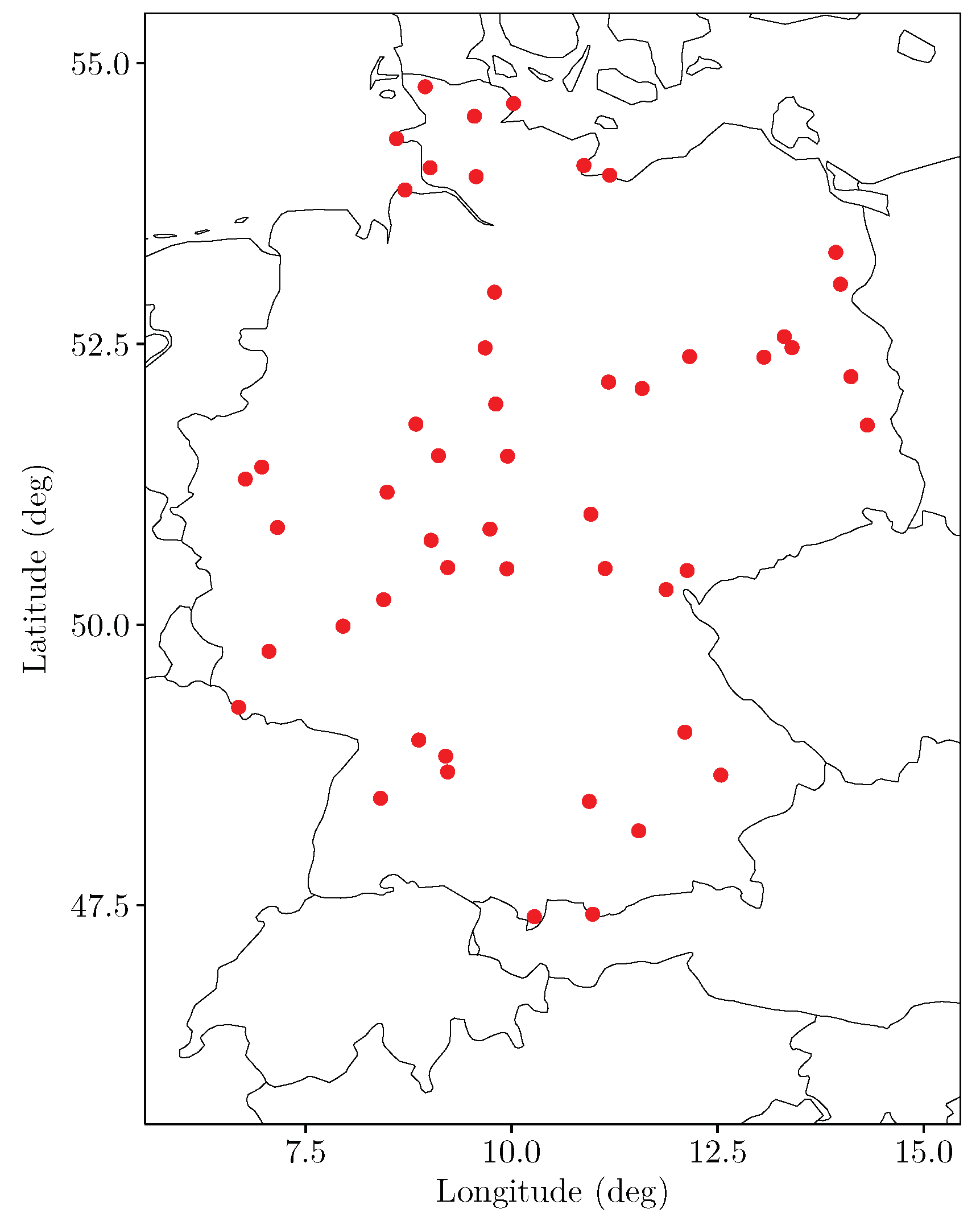
2.2. Data
2.3. Interpolation of Power Curves
2.4. Extrapolation of Power Curves
3. Results
3.1. The Effect of Humidity
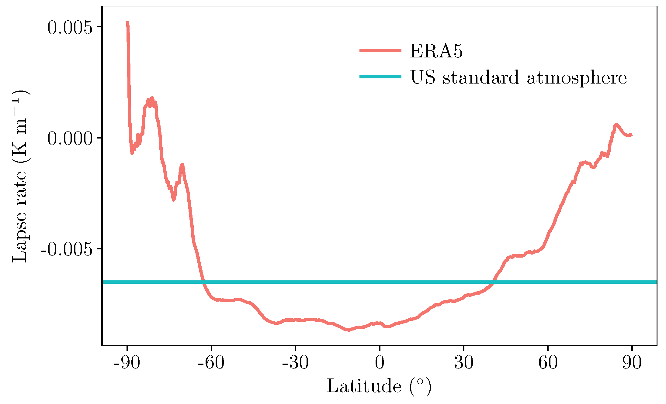
3.2. The Effect of a Varying Lapse Rate
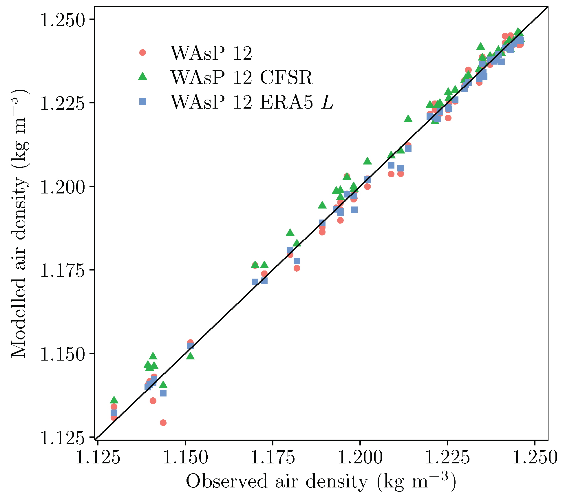
3.3. Using Re-Analysis Outputs
3.4. Example
4. Conclusions and Discussion
Supplementary Materials
Author Contributions
Funding
Acknowledgments
Conflicts of Interest
Abbreviations
| AEP | annual energy production |
| CFSR | climate forecast system re-analysis |
| DTU | Technical University of Denmark |
| ECMWF | European Centre for Medium-Range Weather Forecasts |
| ERA5 | fifth major re-analysis of the European Centre for Medium-Range Weather Forecasts |
| IEC | International Electrotechnical Commission |
| WAsP | Wind Atlas Analysis and Application Program |
References
- Global Wind Energy Council. Global Wind Energy Report: Annual Market Update 2017; Global Wind Energy Council: Bruxelles, Belgium, 2018. [Google Scholar]
- Petersen, E.L.; Mortensen, N.G.; Landberg, L.; Højstrup, J.; Frank, H.P. Wind Power Meteorology. Part I: Climate and Turbulence. Wind Energy 1998, 22, 2–22. [Google Scholar] [CrossRef]
- Petersen, E.L.; Mortensen, N.G.; Landberg, L.; Højstrup, J.; Frank, H.P. Wind Power Meteorology. Part II: Siting and Models. Wind Energy 1998, 1, 55–72. [Google Scholar] [CrossRef]
- Floors, R.; Enevoldsen, P.; Davis, N.; Arnqvist, J.; Dellwik, E. From lidar scans to roughness maps for wind resource modelling in forested areas. Wind Energy Sci. 2018, 3, 353–370. [Google Scholar] [CrossRef]
- Wind Turbines—Part 12-1: Power Performance Measurements of Electricity Producing Wind Turbines; IEC 61400-12-1, Edition 1; IEC–International Electrotechnical Commission: Geneva, Switzerland, 2005.
- Wind Turbines—Part 12-1: Power Performance Measurements of Electricity Producing Wind Turbines; IEC 61400-12-1, Edition 2; IEC–International Electrotechnical Commission: Geneva, Switzerland, 2017.
- Troen, I.; Petersen, E.L. European Wind Atlas; Risø National Laboratory: Roskilde, Denmark, 1989; 656p. [Google Scholar]
- windPRO 3.3 User Manual; EMD International: Aalborg, Denmark, 2019.
- Mortensen, N.G. Wind Resource Assessment Using the WAsP Software; Technical University of Denmark: Roskilde, Denmark, 2016; p. 44. [Google Scholar]
- Saha, S.; Moorthi, S.; Wu, X.; Wang, J.; Nadiga, S.; Tripp, P.; Behringer, D.; Hou, Y.T.; Chuang, H.Y.; Iredell, M.; et al. The NCEP Climate Forecast System Version 2. J. Clim. 2014, 27, 2185–2208. [Google Scholar] [CrossRef]
- Hersbach, H.; Dee, D. ERA5 reanalysis is in production. ECMWF Newsl. 2016, 147, 1. [Google Scholar]
- Stull, R. Practical Meteorology: An Algebra-based Survey of Atmospheric Science; University of British Columbia: Vancouver, BC, Canada, 2017; 940p. [Google Scholar]
- Picard, A.; Davis, R.S.; Gläser, M.; Fujii, K. Revised formula for the density of moist air (CIPM-2007). Metrologia 2008, 45, 149–155. [Google Scholar] [CrossRef]
- Holton, J.R.; Hakim, G.J. An Introduction to Dynamic Meteorology, 4th ed.; Elsevier Academic Press: Cambridge, MA, USA, 2004; p. 535. [Google Scholar]
- United States Committee on Extension to the Standard Atmosphere. U.S. Standard Atmosphere, 1976; National Oceanic and Amospheric [sic] Administration: For Sale by the Superintendent of Documents, U.S. Government Printing Office: Washington, DC, USA, 1976.
- Saha, S.; Moorthi, S.; Wu, X.; Wang, J.; Nadiga, S.; Tripp, P.; Behringer, D.; Hou, Y.T.; Chuang, H.Y.; Iredell, M.; et al. NCEP Climate Forecast System Version 2 (CFSv2) Monthly Products; Research Data Archive at the National Center for Atmospheric Research, Computational and Information Systems Laboratory: Boulder, CO, USA, 2012. [Google Scholar] [CrossRef]
- ERA5: Fifth Generation of ECMWF Atmospheric Reanalyses of the Global Climate. Copernicus Climate Change Service Climate Data Store (CDS). Available online: https://cds.climate.copernicus.eu/cdsapp#!/dataset/reanalysis-era5-single-levels-monthly-means?tab=doc (accessed on 28 May 2019).
- DWD Climate Data Center (CDC). Historical Daily Station Observations (Temperature, Pressure, Precipitation, Sunshine Duration, etc.) for Germany. Available online: ftp://ftp-cdc.dwd.de/pub/CDC/observations_germany/climate/daily/kl/historical/DESCRIPTION_obsgermany_climate_daily_kl_historical_en.pdf (accessed on 28 May 2019).
- Freydank, E. 150 Jahre Staatliche Wetter-und Klimabeobachtungen in Sachsen: Ergänzungs-und Sondernetze, Messungen in der freien Atmosphäre; Institut für Hydrologie und Meteorologie. Available online: https://katalogbeta.slub-dresden.de/id/0-1496504860/ (accessed on 28 May 2019).
- Manwell, J.F.; McGowan, J.G.; Rogers, A.L. Wind Energy Explained; Wiley Online Library: Hoboken, NJ, USA, 2010. [Google Scholar] [CrossRef]
- Svenningsen, L. Proposal of an Improved Power Curve Correction. In Proceedings of the Poster Presented at European Wind Energy Conference, Warsaw, Poland, 20–23 April 2010. [Google Scholar]
- Hudson, S.R.; Brandt, R.E. A Look at the Surface-Based Temperature Inversion on the Antarctic Plateau. J. Clim. 2005, 18, 1673–1696. [Google Scholar] [CrossRef]
- Pachauri, R.K.; Allen, M.R.; Barros, V.R.; Broome, J.; Cramer, W.; Christ, R.; Church, J.A.; Clarke, L.; Dahe, Q.; Dasgupta, P.; et al. Climate Change 2014: Synthesis Report. Contribution of Working Groups I, II and III to the Fifth Assessment Report of the Intergovernmental Panel on Climate Change; IPCC: Geneva, Switzerland, 2014; p. 151. [Google Scholar]


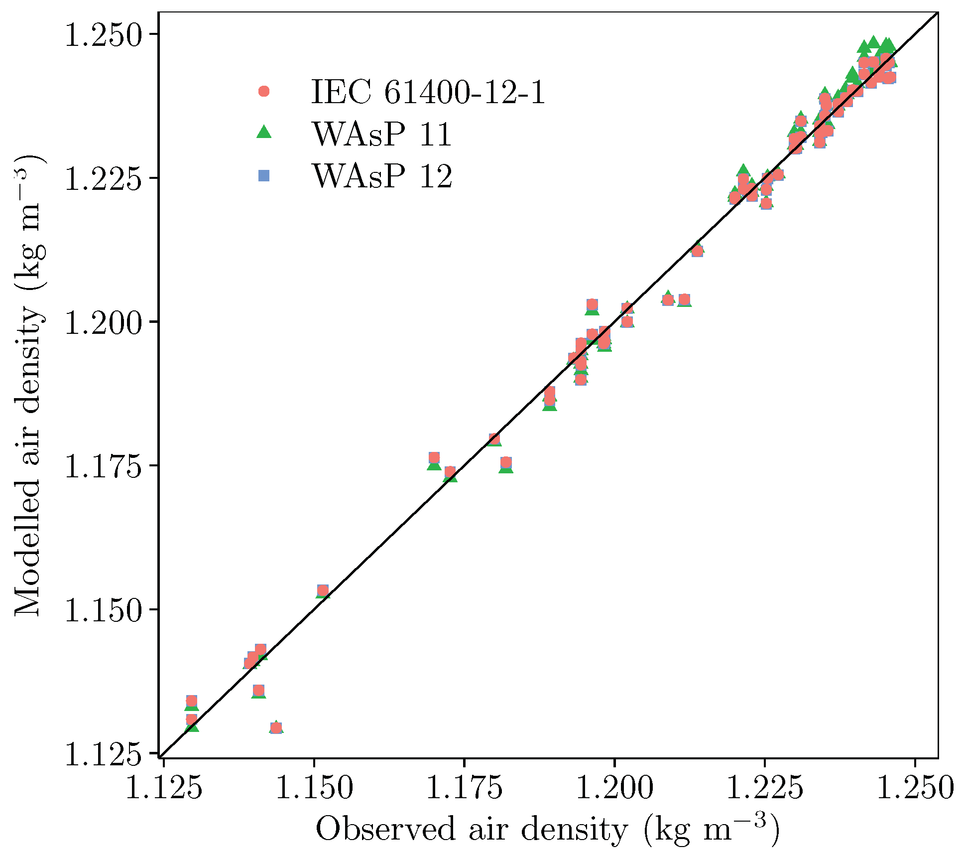
| Method | Mean Abs. Error (%) | R |
|---|---|---|
| WAsP 11 | 0.203 | 0.9975 |
| IEC 61400–12–1 | 0.185 | 0.9977 |
| WAsP 12 | 0.186 | 0.9977 |
| WAsP 12 CFSR | 0.241 | 0.9987 |
| WAsP 12 ERA5 | 0.127 | 0.9993 |
| WAsP 12 ERA5 L | 0.114 | 0.9994 |
| Turbine | [m] | [kg/m3] | [m/s] | Interpol. | Reference Air Density | ||
|---|---|---|---|---|---|---|---|
| 1.12 kg/m | 1.15 kg/m | 1.225 kg/m | |||||
| T4 | 670 | 1.134 | 8.81 | 6716 | 6664 (−0.77%) | 6773 (+0.85%) | 7043 (+4.87%) |
| T8 | 544 | 1.148 | 8.31 | 6416 | 6316 (−1.56%) | 6423 (+0.11%) | 6692 (+4.30%) |
| All | 51,348 | 50,782 (−1.10%) | 51,638 (+0.56%) | 53,782 (+4.74%) | |||
© 2019 by the authors. Licensee MDPI, Basel, Switzerland. This article is an open access article distributed under the terms and conditions of the Creative Commons Attribution (CC BY) license (http://creativecommons.org/licenses/by/4.0/).
Share and Cite
Floors, R.; Nielsen, M. Estimating Air Density Using Observations and Re-Analysis Outputs for Wind Energy Purposes. Energies 2019, 12, 2038. https://doi.org/10.3390/en12112038
Floors R, Nielsen M. Estimating Air Density Using Observations and Re-Analysis Outputs for Wind Energy Purposes. Energies. 2019; 12(11):2038. https://doi.org/10.3390/en12112038
Chicago/Turabian StyleFloors, Rogier, and Morten Nielsen. 2019. "Estimating Air Density Using Observations and Re-Analysis Outputs for Wind Energy Purposes" Energies 12, no. 11: 2038. https://doi.org/10.3390/en12112038
APA StyleFloors, R., & Nielsen, M. (2019). Estimating Air Density Using Observations and Re-Analysis Outputs for Wind Energy Purposes. Energies, 12(11), 2038. https://doi.org/10.3390/en12112038