Implementation and Comparison of Particle Swarm Optimization and Genetic Algorithm Techniques in Combined Economic Emission Dispatch of an Independent Power Plant

Abstract

This paper presents the optimization of fuel cost, emission of NO_X, CO_X, and SO_X gases caused by the generators in a thermal power plant using penalty factor approach. Practical constraints such as generator limits and power balance were considered. Two contemporary metaheuristic techniques, particle swarm optimization (PSO) and genetic algorithm (GA), have were simultaneously implemented for combined economic emission dispatch (CEED) of an independent power plant (IPP) situated in Pakistan for different load demands. The results are of great significance as the real data of an IPP is used and imply that the performance of PSO is better than that of GA in case of CEED for finding the optimal solution concerning fuel cost, emission, convergence characteristics, and computational time. The novelty of this work is the parallel implementation of PSO and GA techniques in MATLAB environment employed for the same systems. They were then compared in terms of convergence characteristics using 3D plots corresponding to fuel cost and gas emissions. These results are further validated by comparing the performance of both algorithms for CEED on IEEE 30 bus test bed.

1. Introduction

The primary objective of an independent electric power producer is to generate electricity at the minimum possible cost. The most expensive commodity in a thermal power plant is the fuel used for the generators to produce electricity. Hence, the focus is on minimizing the production cost; which can be achieved by dispatching the committed generators in the most economical way possible without violating the generators and system electrical constraints and ratings. Moreover, environmental regulatory authorities also impose certain limits on all gas emission sources because of the alarming situation of pollution in the past few decades of many regions around the world [1]. Therefore, a simultaneous minimization of both fuel cost and emission is the obvious way to address those challenges; hence, the idea of a combined economic emission dispatch (CEED) emerged.

Combined dispatch is an efficient and economical solution for decreasing both fuel cost and emission in a thermal power plant without the need to modify the existing system. The simulation gives flexibility to the operator to set the output of generators to achieve a fuel cost benefit for the company and emission allowed by the environmental regulatory authorities. There are many optimization techniques being employed to solve multiobjective problems like CEED. Conventional methods are based on mathematical iterative search which are accurate but time consuming. The nonconventional methods are naturally inspired and give better, if not the best, solution in lesser time as compared to conventional methods. From these artificial-intelligence-based methods, a process of hybridization is going on to accumulate the qualities of individual methods into their hybrids counterparts. This categorization is shown in Figure 1 [2].

Many modern artificial intelligence (AI) techniques based on the theory of Darwinian evolution of biological organisms, e.g., genetic algorithm (GA), and social behaviors of species, e.g., particle swarm optimization (PSO), have been invented. They have been very successful concerning results and regarding dealing with the complexities occurred in formulating such problems. Particle swarm optimization and genetic algorithm are the two leading methods from AI area and are being exploited widely in every discipline including power systems [3,4,5,6]. Their hybrid versions are also reported in the literature [7,8,9], where qualities of both are combined to solve a particular problem. They have also been employed individually on other problems [10,11] where PSO was found to have better performance than that of GA.

In recently reported literature, E. Gonçalves et al. solved nonsmooth CEED using a deterministic approach with improved performance and Pareto curves [1]. They included valve point loading effect but the same approach has to be extended considering other constraints like network losses and prohibited operating zones. H. Liang et al. tackled the multiobjective combined dispatch by developing a hybrid and improved version of bat algorithm [12] and implemented on large scale systems considering power flow constraints. The conducted dispatch was static based on conventional energy resources. B. Lokeshgupta et al. proposed a combined model of multiobjective dynamic economic and emission dispatch (MODEED) and demand side management (DSM) technique using multiobjective particle swarm optimization (MOPSO) algorithm and validated their results via three different cases studied on a six unit test system [13] and can be extended towards distributed generation in microgrids.

In reported literature [14,15,16], in most cases, only one technique has been used to solve CEED on IEEE test cases, and their results have been compared with previous work. In

Table 1. Best optimization methods employed in different systems with regard to cost, emission, and time

No.	System	Cost-effective	Emission-effective	Time-effective
1.	1 power unit, 2 cogeneration units, and 1 heat unit	Harmony search and genetic algorithm (HSGA)	X	Cuckoo search algorithm (CSA)
		Nondominated sorting genetic algorithm (NSGA-II)	Nondominated sorting genetic algorithm (NSGA-II)	Nondominated sorting genetic algorithm (NSGA-II)
2.	1 power unit, 3 cogeneration units, and 1 heat unit	HSGA	X	Gravitational search algorithm (GSA)
3.	4 thermal generators, 2 cogeneration units, and 1 heat unit	GSA	X	Effective cuckoo search algorithm (ECSA)
		Grey wolf optimization (GWO)	GWO	GWO
4.	13 power units, 6 cogeneration units, and 7 heat units	Exchange market algorithm (EMA)	X	Modified particle swarm optimization (MPSO)
5.	26 power units, 12 cogeneration units, and 10 heat units	MPSO	X	MPSO

, the survey of [17] is summarized to conclude that GA is better for low-power systems while PSO outperforms in the case of high-power systems. However, what happens when these two leading metaheuristic techniques are employed together to the same system? This work deals with this novel idea, hence, both PSO and GA will be implemented individually on CEED of an independent power plant (IPP) situated in Pakistan considering all gases (NO_X, CO_X, and SO_X) for various load demands. The results will be of great importance as the data of an actual IPP will be utilized and they will also grade the performance of PSO and GA for CEED of an IPP. In order to validate the results, a conventional IEEE 30 bus system is also considered. This work will contribute the results of combined dispatch of fuel and gas emissions (economic and environmental aspects, respectively) carried out on a power plant with two leading algorithms (PSO and GA) using MATLAB and then comparing their performance in terms of better solution, convergence characteristics (3D plots), and computation time. The implementation, comparison, and convergence characteristics of PSO and GA employed for the same systems are the main contribution of this work to the field. These characteristics were compared with each other with 3D plots to analyze the better solution yielded by the two algorithms applied for CEED of the same systems in MATLAB environment.

2. Problem Formulation

CEED comprises two objective functions (cost and emission) that are to be minimized. The fuel cost and emission of a generator can be represented as a quadratic function of the generator’s real power [18]. Hence, for N running generators in a plant, the total fuel cost (FC) and emission of a single gas (E_g), respectively, are given in Equations (1) and (2).

$$FC={\displaystyle \sum }_{i=1}^N{F}_i\left(P_i\right)={\displaystyle \sum }_{i=1}^N\left(a_i{P}_i^2+b_i{P}_i+c_i\right)$$

(1)

$$E_g={\displaystyle \sum }_{i=1}^N{E}_i\left(P_i\right)={\displaystyle \sum }_{i=1}^N\left({\alpha }_i{P}_i^2+{\beta }_i{P}_i+{\gamma }_i\right)$$

(2)

where a_i, b_i, and c_i are cost coefficients; α_i, β_i, and γ_i are emission coefficients of unit i out of N generators. They are computed by the following:

• Getting the heat rate curves and emission reports of operational generators from the plant.
• Then, calculating and arranging their fuel costs and emissions corresponding to their active powers in tabular form.
• Applying the quadratic curve fitting technique on these data points to get cost and emission coefficients.

This multiobjective optimization problem is converted to a single objective function of total cost (TC) by imposing a penalty (h_g) on the emission of G gases to convert them into emission cost (EC).

$$TC=FC+EC=FC+{\displaystyle \sum }_{g=1}^G{h}_g\times E_g$$

(3)

There are different types of penalty factors; their benefits and drawbacks are thoroughly discussed in [19]. The min–max penalty factor of Equation (4) is used in this work because of its superiority reported in [19] over the others.

$$h_i=\frac{F_i\left(P_{i,min}\right)}{E_i\left(P_{i,max}\right)}=\frac{a_i{P}_{i,min}^2+b_i{P}_{i,min}+c_i}{{\alpha }_i{P}_{i,max}^2+{\beta }_i{P}_{i,max}+{\gamma }_i}$$

(4)

where h_i for each generator for every gas is calculated and all are sorted in ascending order, then starting from the smallest h_i, P_i,max of corresponding generator is added until ${\displaystyle \sum }{P}_{i,max}\ge P_D$, the h_i at this stage is selected as penalty factor h_g of that gas for the given load demand.

For achieving this optimization, the N generators will be dispatched with various combinations of output powers but each combination must conform to two mandatory constraints. First of all, no unit should violate its limits for producing output power (P_i), and secondly the total generation (P_G) should meet the load demand (P_D) and transmission line losses (P_L) [18].

$$P_{i,min}\le P_i\le P_{i,max}$$

(5)

$$P_G={\displaystyle \sum }_{i=1}^N{P}_i=P_D+P_L$$

(6)

The generator limits constraint is satisfied by initializing each unit’s power within prescribed limits and then constantly checking the violation. If a unit crosses its limit, then its output is set to that limit. The second power balance constraint is accounted for by letting algorithm to find optimal powers for N − 1 generators and setting the power (P_N) of last generator N also called slack generator to:

$$P_N=(P_D+P_L)-{\displaystyle \sum }_{i=1}^{N-1}{P}_i$$

(7)

If losses are ignored, then the power of slack generator will reduce to:

$$P_N=P_D-{\displaystyle \sum }_{i=1}^{N-1}{P}_i$$

(8)

3. Implementation of PSO to CEED

J. Kennedy and R. Eberhart proposed this method in 1995 after observing and modeling the social interaction within bird flocks and fish schools for searching food [20]. The particles in such swarms move to attain optimal objective (food) based on their personal (pbest) and swarm’s (gbest) best experiences. Each particle is a valid solution to the problem, and hence, its dimension is that of problem space. The position of each particle keeps on updating by its current velocity, particle’s best position, and swarm’s best position until the optimal solution is discovered. The velocity and position of the particle is given by Equations (9) and (10).

$$v_j^{k+1}={\mu }^k{v}_j^k+c_1{r}_1\left(pbes{t}_j-x_j^k\right)+c_2{r}_2\left(gbest-x_j^k\right)$$

(9)

$$x_j^{k+1}=x_j^k+v_j^{k+1}$$

(10)

where j is particle counter, k is iteration counter, c₁ and c₂ are acceleration coefficients, r₁ and r₂ are random numbers in the range of 0–1, pbest_j is the best position of particle based on its personal knowledge, gbest is the best position of particle based on group knowledge, and μ is the inertia weight given by Equation (11).

$${\mu }^k={\mu }_{max}-\left(\frac{{\mu }_{max}-{\mu }_{min}}{ite{r}_{max}}\right)k$$

(11)

The performance of classical PSO has been made a lot better by working on its various parameters and by using different search strategies for updating the particle’s position [18]. Hence, different variants of PSO has been introduced, such as WIPSO and TVAC-PSO, in which inertia weight μ is improved and acceleration coefficients c₁ and c₂ are timely varied [21], MRPSO [22] in which particle’s position is changed by using moderate random and chaotic search techniques, respectively. It has been observed that the most straightforward and efficient way of making classical PSO more effective is to use the constriction factor approach (CFA) [23], in which particle’s velocity (9) is multiplied by a parameter called constriction factor (CF) given by Equation (12).

$$CF=\frac{2}{\left|2-\phi -\sqrt{{\phi }^2-4\phi }\right|}$$

(12)

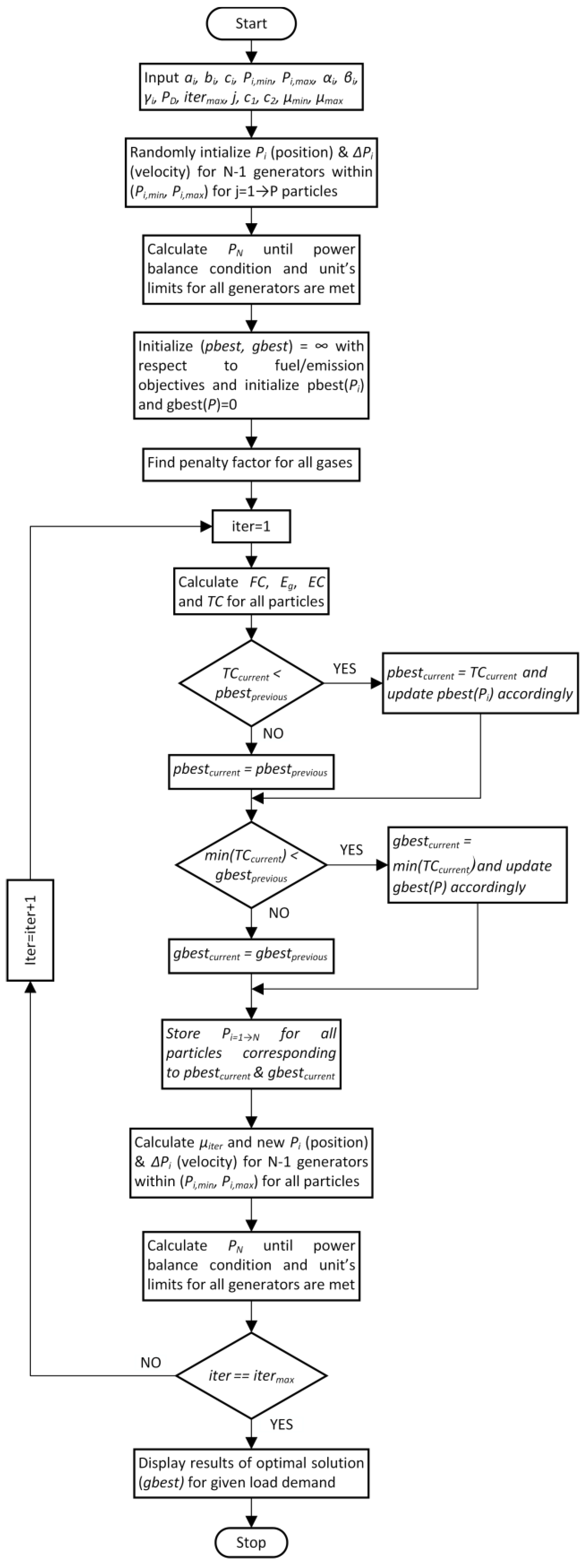
where φ = c₁ + c₂ and φ > 4. The PSO algorithm for CEED, with corresponding flowchart in Figure 2, is implemented in the following steps:

• Input values of fuel coefficients, generators limits, emission coefficients, load demand, maximum iterations, number of particles, acceleration coefficients, and inertia weight’s maxima-minima.
• Randomly initialize power outputs (position) of N − 1 generators within their limits and change in these powers (velocity) for all particles.
• Calculate the power of slack generator from Equation (8) to meet the power balance condition of Equation (6). P_N should also be within its unit’s limits. If any unit out of N surpasses its boundary at any stage throughout the algorithm, it is set to the limit which it has broken.
• Initialize pbest and gbest to infinity and find penalty factors of all considered gases.
• Find fuel cost FC, emission of gases E_g, emission cost EC with total cost TC for all particles from Equations (1)–(3), respectively.
• Update pbest of each particle with its total cost if former is greater than latter. The minimum pbest out of all particles is stored as gbest if its present value is smaller than its previous value. The generators’ powers corresponding to pbest and gbest are stored in separate matrices and are also modified on every update.
• Calculate inertia weight from Equation (11), find new velocities and positions of N-1 generators for all particles form Equations (9) and (10), and keep them within units’ limits in case of violation.
• For slack generator N, calculate its power from Equation (8) and this should also be in limits. If violation is done, set this power to the limit crossed and start changing the output from first generator until Equations (5) and (6) are satisfied.
• If algorithm is converged, continue to next step, go to step 5 otherwise.
• Print neatly the results of optimal solution (gbest) including powers of all generators, line losses, fuel cost, emission of gases, penalty factors, emission cost, and total cost for the given load demand.

4. Implementation of GA to CEED

D.E. Goldberg gave the basic theory for design and analysis of genetic algorithms based on the concept of biological evolution in 1988–1989 [24], and later, J.H. Holland established it systematically as a fact. In genetic algorithms, the problem variables (output powers) are coded into binary strings. Each string is a valid solution to the problem and hence its length should be comparable to the problem space (number of generators N). The bits reserved logically for single generator’s power (genbits) in a string is given in Equation (13).

$$2^{genbits}\ge Max\left[P_{1,max},P_{N,max}\right]$$

(13)

The length of the binary string (strlen) will be $N\times genbits$. Each individual (string) has a fitness value in the range 0–1 which basically relates that individual to the one having maximum fitness in that population. The fitness function should be linked to the objective under discussion contrary to the constraints of the objective function which should be dealt by external checks. Considering this fact and the remarkable communication within the group by PSO parameters pbest and gbest, a new fitness function different from the one reported in [3] and [5] for jth individual out of P individuals is given by (14).

$$fi{t}_j=1-\left(\frac{pbes{t}_j-gbest}{Max\left[pbes{t}_1,pbes{t}_P\right]-gbest}\right)$$

(14)

The initial population is randomly generated, keeping in view the generators’ limits but the next generations are produced by selection, crossover, and mutation performed on the present one (powers corresponding to pbest). Selection is basically making a mating pool of fitter strings from present population based on the natural principle of “survival of the fittest.” It is usually done by the concept of roulette-wheel. No new string is formed in selection phase. The greater the fitness of a string, the greater portion of the wheel’s circumference it will occupy and the greater chance it will get to copy into mating pool. The wheel is spun P times to select a population of good parents for producing off springs by crossover and mutation.

Crossover is performed on two parents of selected population to produce two off springs. There are three types of crossover: one point, multi-point, and uniform, explained in

Table 2. The types of crossover.

Item	One Point	Multipoint	Uniform
Parent 1	000 00000	00 00 00 00	00 00 00 00
Parent 2	111 11111	11 11 11 11	11 11 11 11
Site/Mask	3	2, 4, 6	01 01 10 10
Child 1	000 11111	00 11 00 11	01 01 10 10
Child 2	111 00000	11 00 11 00	10 10 01 01

.

Crossover site is selected randomly and the probability of crossover (p_c) is usually taken higher. In this work, one point crossover is performed on selected strings of mating pool. Finally, mutation is performed on the children produced after crossover which is just flipping of the child’s bit at mutation site selected randomly. Its probability (p_m) is usually taken lower, e.g., if child is (11 11 11 11) and mutation site is 4, then the mutated child will be (11 10 11 11). This journey of producing next generations continues until the optimum solution is found.

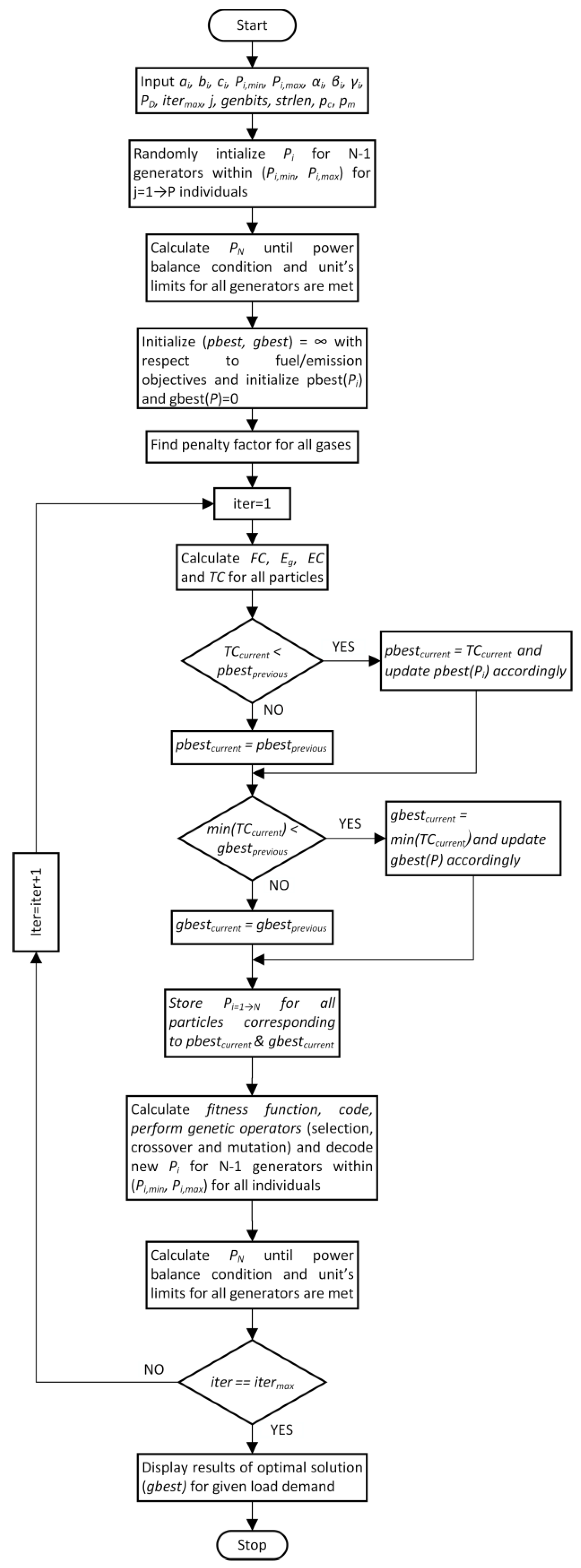
The GA algorithm for CEED, with corresponding flowchart in Figure 3, is implemented in the following steps:

• Input values of fuel coefficients, generators limits, emission coefficients, load demand, maximum iterations, number of individuals, genbits from Equation (13), strlen, p_c, and p_m.
• Randomly initialize power outputs of N−1 generators within their limits for all individuals.
• Calculate the power of slack generator from Equation (8) to meet power balance condition of Equation (6). P_N should also be within its unit’s limits. If any unit out of N surpasses its boundary at any stage throughout the algorithm, it is set to the limit which it has broken.
• Initialize pbest and gbest to infinity and find penalty factors of all considered gases.
• Find fuel cost FC, emission of gases E_g, emission cost EC with total cost TC for all particles from Equations (1)–(3), respectively.
• Update pbest of each individual with its total cost if former is greater than latter. The minimum pbest out of all particles is stored as gbest if its present value is smaller than its previous value. The generators’ powers corresponding to pbest and gbest are stored in separate matrices and are also modified on every update.
• Calculate fitness function for all individuals from Equation (14). Code the output powers to binary strings, perform the three genetic operators (selection, crossover, and mutation), and again decode them to output powers.
• Keep all outputs within units’ limits in case of violation. For slack generator N, calculate its power from Equation (8), and this should also be in limits. If violation is done, set this power to the limit crossed and start changing the output from first generator until Equations (5) and (6) are satisfied.
• If algorithm is converged, continue to next step, go to step 5 otherwise.
• Print neatly the results of optimal solution (gbest) including powers of all generators, line losses, fuel cost, emission of gases, penalty factors, emission cost, and total cost for the given load demand.

5. Simulation Results

Combined economic emission dispatch using PSO and GA for 500 iterations were implemented on MATLAB on six generators of IEEE 30 bus system and eight committed units (gas turbines) of an IPP in Pakistan for load demands of 1500 and 2000 MW, and 500 and 700 MW, respectively. The initial parameters set in both algorithms were:

• PSO: Particles = 10, μ_max = 0.9, μ_min = 0.4, c₁ = 2.05, c₂ = 2.05, φ = 4.1, and CF = 0.7298
• GA: Individuals = 10, p_c = 0.96, and p_m = 0.033

The solutions with average operating time (t) were selected out of 50 trials for comparison between PSO and GA.

5.1. IEEE 30 Bus System

The data for fuel cost and emission coefficients were taken from [5]. Transmission line losses were not accounted for while all three gases (NO_X, CO_X, and SO_X) were considered; their penalty factors were calculated using Equation (4) and the procedure following this equation, for load demands of 1500 and 2000 MW given as:

• P_D = 1500 MW: h_NOX = 3.1669, h_COX = 0.1221, and h_SOX = 0.9182
• P_D = 2000 MW: h_NOX = 5.7107, h_COX = 0.1307, and h_SOX = 0.9850

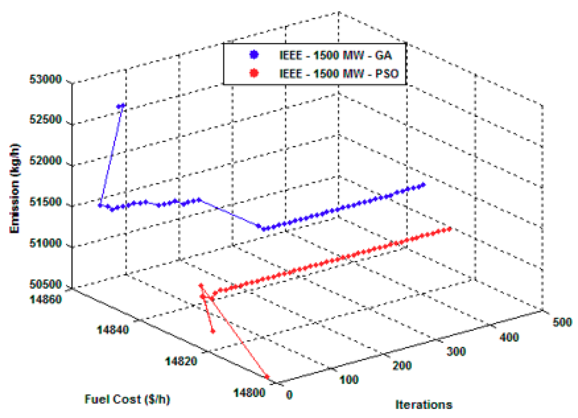
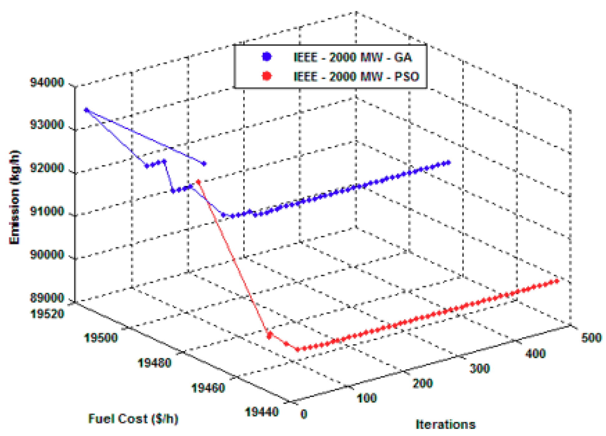
The results are summarized in

Table 3. The real-time simulation results of PSO and GA for IEEE 30 bus system with P_D = 1500 MW and P_D = 2000 MW.

Case A		P1	P2	P3	P4	P5	P6	ENOX	ECOX	ESOX	E	EC	FC	TC	t
PD = 1500 MW	PSO	195.79	256.55	381.25	81.69	381.85	202.27	1719.67	39,626.51	9623.04	50,969.21	19,121.26	14,827.57	33,948.83	0.1326
	GA	196	255	351	79	416	203	1731.52	40,049.21	9579.83	51,360.56	19,170.74	14,835.04	34,005.78	0.4528
PD = 2000 MW	PSO	256.32	320.57	541.95	133.1	500	248.06	2540.68	73,738.76	13,601.05	89,880.5	37,543.01	19,445.29	56,988.3	0.1227
	GA	268	287	562	127	500	256	2537.8	75,505.33	13,450.06	91,493.19	37,608.68	19,485.44	57,094.12	0.4706

(all powers are in MW, emissions in kg/h, costs in $/h, and time in seconds) while the convergence characteristics of both algorithms, with respect to both objectives (fuel cost and emission) for P_D = 1500 MW and P_D = 2000 MW, are shown in Figure 4 and Figure 5, respectively.

5.2. Pakistani IPP

This thermal power plant comprises of 15 generating units out of which 10 are multi-fuel-fired gas turbines and remaining five are steam turbines with an overall capacity of 1600 MW. The combined dispatch was performed on eight gas turbines as the remaining two are uneconomical and mostly turned off. Steam turbines take exhaust of gas turbines to operate, hence they were not considered as they do not take any direct fuel.

The data calculated and used for the dispatch of all units is given in Appendix A. Transmission line losses were ignored because IPP’s main concern is generation capacity which they have to produce and supply to national grid, and SO_X gas were not accounted for because of the unavailability of sufficient data. Remaining two gases (NO_X and CO_X) were considered; their penalty factors were calculated using Equation (4) and the procedure following this equation, for load demands of 500 and 700 MW given as:

• P_D = 500 MW: h_NOX = 1.5751, h_COX = 101.1369
• P_D = 700 MW: h_NOX = 1.7218, h_COX = 123.8797

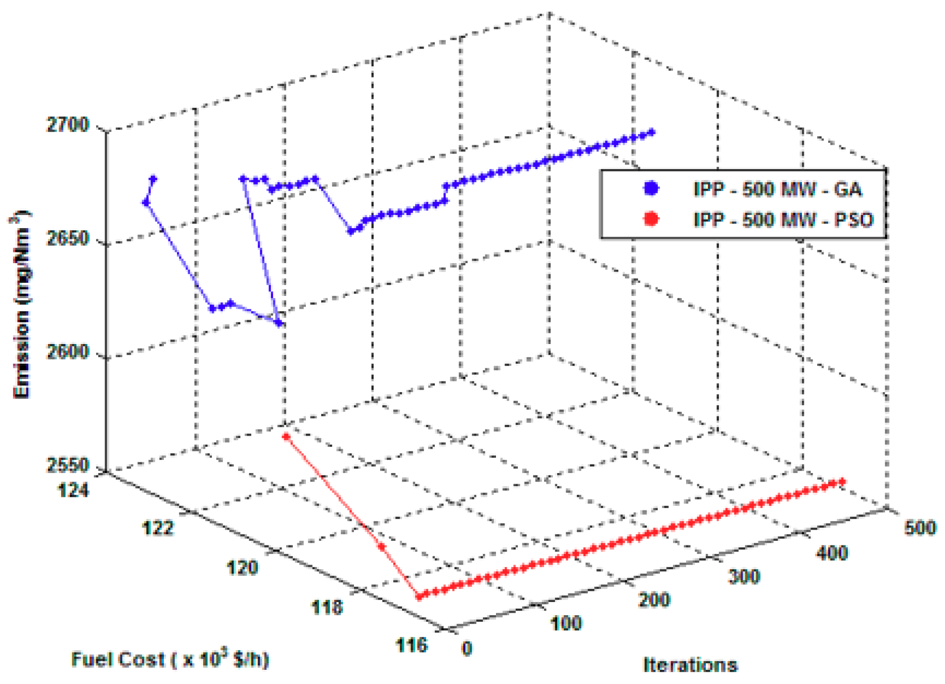
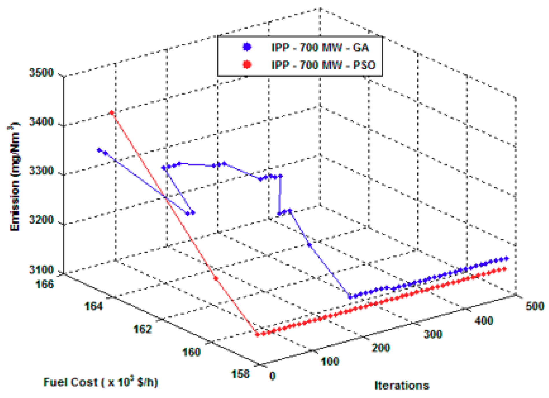
The results are summarized in

Table 4. The real-time simulation results of PSO and GA for Pakistani independent power plant (IPP) with P_D = 500 MW and P_D = 700 MW.

Case B		P1	P2	P3	P4	P5	P6	P7	P8	ENOX	ECOX	E	EC	FC	TC	t
PD = 500 MW	PSO	32.5	32.5	100	90.87	83.68	100	25	35.44	2512.49	40.04	2552.53	76	117.1	193.1	0.1531
	GA	33	32.5	32	92	96	100	64	50.5	2624.22	43.32	2667.54	80.82	121.6	202.42	0.8031
PD = 700 MW	PSO	130	130	100	90.83	83.82	100	25	40.35	3093.41	48.93	3142.35	108.09	158.5	266.59	0.1509
	GA	130	130	100	87	96	100	25	32	3110.72	55.41	3166.13	115.1	158.4	274.4	0.5411

(all powers are in MW, emissions in mg/Nm³, costs in 10³ $/h, and time in seconds) while the convergence characteristics of both algorithms, with respect to both objectives (fuel cost and emission) for P_D = 500 MW and P_D = 700 MW, are shown in Figure 6 and Figure 7, respectively.

6. Results Discussion

In Table 3, the power output of all six generators was presented as the sum of which is equal to the load demand (1500 and 2000 MW) for both algorithms (PSO and GA). Then, the emissions of all three gases (NO_X, CO_X, SO_X) from these generators were calculated and added (E) to convert into cost (EC) using penalty factor approach. The fuel cost (FC) is calculated from the generators’ powers and is added to the emission cost to achieve total cost (TC) of the combined dispatch. In the end, the given time (t) represents the computational time of the algorithm for that particular load demand and PSO produces the optimal solution 4 times quicker than that of GA for both load demands. Figure 4 shows the 3D plot of fuel cost and emission with regard to iterations for 1500 MW. It shows that PSO starts with lower fuel cost and emission, and converges quickly on the optimal solution as compared to GA which starts with higher fuel cost and emission and takes some time to converge. Figure 5 shows the similar 3D plot but for a load demand of 2000 MW in which PSO gets lost for a small time period in non-optimized region but quickly converges on the solution with lower fuel cost and emission, while GA converges in steps on to a solution which is not better than PSO.

Table 4 gives the output power of eight gas-fired generators and this total generation is equal to the load demand (500 and 700 MW) for both cases (PSO and GA). From the generators’ powers, the fuel cost (FC) and emission of two gases (NO_X and CO_X) were calculated using quadratic relation of generator’s output to fuel cost and emission, respectively. The emission was then totaled (E) and converted to cost (EC) by imposing penalty factor. These two costs (related to fuel and emission) were then added to get total cost (TC) of the combined dispatch of the power plant. In the end, t is the time taken by each algorithm to carry out the dispatch for a particular load demand. It is noteworthy that PSO is 4–7 times faster than its GA counterpart for both load demands. Figure 6 shows the 3D plot of fuel cost and emission with regard to iterations for 500 MW. In this figure, PSO starts with higher fuel cost but in few iteration, it converges on the optimal solution while GA remains stuck in non-optimized region. Figure 7 shows the similar 3D plot but for a load demand of 700 MW. In this simulation, both PSO and GA starts from nearby solutions, but then, PSO converges very quickly while GA struggles up to 300 iterations and then converges to a nearer solution of PSO, but still, this solution is not better than the one provided by PSO.

7. Conclusions

The combined dispatch of plant generators with respect to fuel and gas emissions was carried out using PSO and GA in MATLAB. The results demonstrate that PSO outperforms GA for the combined dispatch in terms of achieving lower fuel cost, lower emission, fast convergence, and lesser simulation time. This was validated for both IEEE 30 bus system and for an independent power plant with simulation, 3D plots, and thorough discussion. The work has successfully implemented PSO and GA algorithms for CEED of the same systems. The simulation results are compared and tabulated for different load demands. 3D plots were discussed to highlight the convergence characteristics of PSO and GA with respect to fuel cost and gas emissions. In future studies, the combined dispatch will be made more realistic, by including some other practical constraints like valve point loading, ramp rate limits, prohibited operating zones of generators, transmission line losses etc. The algorithms, PSO and GA, can be made more efficient by studying and improving their performance parameters.

References

- Gonçalves, E.; Roberto Balbo, A.; da Silva, D.N.; Nepomuceno, L.; Baptista, E.C.; Soler, E.M. Deterministic approach for solving multi-objective non-smooth Environmental and Economic dispatch problem. Int. J. Electr. Power Energy Syst. 2019, 104, 880–897. [Google Scholar]
- Mahdi, F.P.; Vasant, P.; Kallimani, V.; Watada, J.; Siew Fai, P.Y.; Abdullah-Al-Wadud, M. A holistic review on optimization strategies for combined economic emission dispatch problem. Renew. Sustain. Energy Rev. 2018, 81, 3006–3020. [Google Scholar] [CrossRef]
- Mishra, S.K.; Mishra, S.K. A comparative study of solution of economic load dispatch problem in power systems in the environmental perspective. Proc. Comput. Sci. 2015, 48, 96–100. [Google Scholar] [CrossRef][Green Version]
- Kothari, D.P. Power system optimization. In Proceedings of the 2012 2nd National Conference on Computational Intelligence and Signal Processing (CISP), Guwahati, Assam, India, 2–3 March 2012. [Google Scholar]
- AlRashidi, M.R.; El-Hawary, M.E. Emission-economic dispatch using a novel constraint handling particle swarm optimization strategy. In Proceedings of the 2006 Canadian Conference on Electrical and Computer Engineering, Ottawa, ON, Canada, 7–10 May 2006. [Google Scholar]
- Bora, T.C.; Mariani, V.C.; dos Santos Coelho, L. Multi-objective optimization of the environmental-economic dispatch with reinforcement learning based on non-dominated sorting genetic algorithm. Appl. Therm. Eng. 2019, 146, 688–700. [Google Scholar] [CrossRef]
- Ghamisi, P.; Benediktsson, J.A. Feature selection based on hybridization of genetic algorithm and particle swarm optimization. IEEE Geosci. Remote Sens. Lett. 2015, 12, 309–313. [Google Scholar] [CrossRef]
- Jiang, H.; Zhang, Y.; Xu, H. Optimal allocation of cooperative jamming resource based on hybrid quantum-behaved particle swarm optimisation and genetic algorithm. IET Radar Sonar Navig. 2016, 11, 185–192. [Google Scholar] [CrossRef]
- Wang, J.; Zhang, F.; Liu, F.; Ma, J. Hybrid forecasting model-based data mining and genetic algorithm-adaptive particle swarm optimisation: A case study of wind speed time series. IET Renew. Power Gener. 2016, 10, 287–298. [Google Scholar] [CrossRef]
- Ohatkar, S.N.; Bormane, D.S. Hybrid channel allocation in cellular network based on genetic algorithm and particle swarm optimisation methods. IET Commun. 2016, 10, 1571–1578. [Google Scholar] [CrossRef]
- Villarroel, R.D.; García, D.F.; Dávila, M.A.; Caicedo, E.F. Particle swarm optimization vs genetic algorithm, application and comparison to determine the moisture diffusion coefficients of pressboard transformer insulation. IEEE Trans. Dielectr. Electr. Insul. 2015, 22, 3574–3581. [Google Scholar] [CrossRef]
- Liang, H.; Liu, Y.; Li, F.; Shen, Y. A multiobjective hybrid bat algorithm for combined economic/emission dispatch. Int. J. Electr. Power Energy Syst. 2018, 101, 103–115. [Google Scholar] [CrossRef]
- Lokeshgupta, B.; Sivasubramani, S. Multi-objective dynamic economic and emission dispatch with demand side management. Int. J. Electr. Power Energy Syst. 2018, 97, 334–343. [Google Scholar] [CrossRef]
- Güvenç, U.; Sönmez, Y.; Duman, S.; Yörükeren, N. Combined economic and emission dispatch solution using gravitational search algorithm. Sci. Iranica 2012, 19, 1754–1762. [Google Scholar]
- Jebaraj, L.; Venkatesan, C.; Soubache, I.; Christober Asir Rajan, C. Application of differential evolution algorithm in static and dynamic economic or emission dispatch problem: A review. Renew. Sustain. Energy Rev. 2017, 77, 1206–1220. [Google Scholar] [CrossRef]
- Niu, Q.; Zhang, H.; Wang, X.; Li, K.; Irwin, G.W. A hybrid harmony search with arithmetic crossover operation for economic dispatch. Int. J. Electr. Power Energy Syst. 2014, 62, 237–257. [Google Scholar] [CrossRef]
- Nazari-Heris, M.; Mohammadi-Ivatloo, B.; Gharehpetian, G. A comprehensive review of heuristic optimization algorithms for optimal combined heat and power dispatch from economic and environmental perspectives. Renew. Sustain. Energy Rev. 2018, 81, 2128–2143. [Google Scholar] [CrossRef]
- Mahor, A.; Prasad, V.; Rangnekar, S. Economic dispatch using particle swarm optimization: A review. Renew. Sustain. Energy Rev. 2009, 13, 2134–2141. [Google Scholar] [CrossRef]
- Krishnamurthy, S.; Tzoneva, R. Investigation on the impact of the penalty factors over solution of the dispatch optimization problem. In Proceedings of the 2013 IEEE International Conference on Industrial Technology (ICIT), Cape Town, South Africa, 25–28 February 2013. [Google Scholar]
- Kennedy, J. Particle swarm optimization. Encycl. Mach. Learn. 2010, 760–766. [Google Scholar] [CrossRef]
- Vu, P.; Dinh Le, L.; Vo, N.; Tlusty, J. A novel weight-improved particle swarm optimization algorithm for optimal power flow and economic load dispatch problems. In Proceedings of the IEEE PES T&D 2010, New Orleans, LA, USA, 19–22 April 2010. [Google Scholar]
- Singh, N.; Kumar, Y. Economic load dispatch with environmental emission using MRPSO. In Proceedings of the 2013 3rd IEEE International Advance Computing Conference (IACC), Ghaziabad, India, 22–23 February 2013. [Google Scholar]
- Dasgupta, K.; Banerjee, S. An analysis of economic load dispatch using different algorithms. In Proceedings of the 2014 1st International Conference on Non Conventional Energy (ICONCE 2014), Kalyani, India, 16–17 January 2014. [Google Scholar]
- Goldberg, D.E.; Holland, J.H. Genetic algorithms and machine learning. Mach. Learn. 1988, 3, 95–99. [Google Scholar] [CrossRef]
© 2019 by the authors. Licensee MDPI, Basel, Switzerland. This article is an open access article distributed under the terms and conditions of the Creative Commons Attribution (CC BY) license (http://creativecommons.org/licenses/by/4.0/).