Reliability Based Genetic Algorithm Applied to Allocation of Fiber Optics Links for Power Grid Automation

Abstract

In this work, we address the problem of allocating optical links for connecting automatic circuit breakers in a utility power grid. We consider the application of multi-objective optimization for improving costs and power network reliability. To this end, we propose a novel heuristic for attributing reliability values to the optical links, which makes the optimization converge to network topologies in which nodes with higher power outage indexes receive greater communication resources. We combine our heuristic with a genetic algorithm in order to solve the optimization problem. In order to validate the proposed method, simulations are carried out with real data from the local utility. The obtained results validate the allocation heuristic and show that the proposed algorithm outperforms gradient descent optimization in terms of the provided Pareto front.

1. Introduction

The increasingly stringent requirements imposed on energy utilities imply greater investments by these companies in their main infrastructure. Such requirements are related to quality of service regulation by supervising agencies, which forces companies to invest in technologies that enable the operation of their grids according to established standards. Among the parameters whose observance is solicited by the utilities, there are continuity indexes, which measure quality of service in terms of frequency and duration associated with blackout events registered in the distribution grid [1,2].

The attainment of adequate continuity indexes is associated with investments in automation mechanisms for the distribution grid. Intensely automated grids belong to the smart grid classification, which, among other characteristics, refers to power grids capable of operation and fault clearing during complex contingency situations, without the need for human assistance. In particular, the automation of breakers is very important, since it allows rapid supply reestablishment after the correction of faults along the distribution grid [3].

In this work, we consider the problem of optimizing the allocation of fiber optics links for connecting automatic breakers in a distribution grid. The optimization objective is to attain high reliability for breaker operation and, thus, improvement of supply quality perceived by consumers connected to the grid. It is assumed that the breakers communicate via fiber optics, whose allocation must reflect a compromise between reliability and cost. Results concerning the number of feasible solutions are established, suggesting the use of a genetic algorithm as adequate for the problem. A proposed allocation heuristic is incorporated into the objective function evaluation during the optimization process. Solution constraints that contemplate limitations associated with the physical problem are also considered.

This paper is organized as follows. In Section 2, we briefly review previous works regarding reliability optimization of automated power grids. In Section 3, we discuss the objective functions and constraints inherent to the problem. A simple method for estimating reliability with significantly reduced computational complexity is proposed. Furthermore, we propose a heuristic for attributing reliability values to optical links in order to improve the distribution of reliability gains throughout the power grid. In Section 4, we contemplate possible solution methods for the problem and conclude that using a genetic algorithm is the best option. In Section 5, we present results obtained in a case study, which was carried out by applying the proposed methods to real data of the local distribution utility.

2. Related Works

The increase in interest in implementing smart grids has given rise to multiple solutions regarding the reliable operation of automated grids. The design of communication links associated with automated grid elements and the adequate allocation of distributed generation are problems associated with modern grids. In these scenarios, reliability measures attributed to grid service become dependent on the distributed power sources and failure rates of the communication links [4].

In this sense, power grid control and planning are submitted to a great number of stringent operation criteria that must be satisfied simultaneously. As a consequence, a recent trend in power systems research is the application of heuristics and multi-objective algorithms for optimizing modern grids with respect to reliability and other quality parameters. This procedure is convenient for grid management, since it contemplates multiple opposing parameters and extends the decision-making process by providing a set of optimal solutions.

The optimization of power dispatch and allocation of distributed generation has been considered in recent works from the viewpoint of various grid quality parameters. In [5], the control parameters of distributed DC-AC inverters were optimized to improve grid stability and power sharing. In [6], the reconfiguration strategy of grid switches was considered for simultaneously optimizing power losses, voltage deviation, and service outage. In [7], optimization of equipment cost and service reliability was achieved by optimizing the allocation of distributed generation and reconnecting switches.

Other works carried out multi-objective optimization considering external factors impacted by power system operation. In [8], a genetic algorithm was used to optimize power dispatch in order to minimize fuel costs and ambient impact due to gas emission by thermal units. Similarly, evolutionary algorithms were applied in [9] for optimizing polluting gas emission, grid voltage deviation, and active power losses. In [10], the ant-lion optimization heuristic was applied to distributed generation allocation to achieve optimal combinations of investment benefit, power losses, and voltage stability.

The above works considered system reliability as a function of power dispatch and allocated distributed generation. However, reliability associated with smart grid communication networks is of a different nature. The former provide knowledge concerning the grid capacity for consumer demand coverage, whereas the latter represent guarantees of appropriate automation triggering if a fault occurs. Hence, reliability measures related to communication networks must consider failure rates associated with the power feeders, which are measured by historical records of grid power outages.

Many recent works have considered the problem of planning the communication infrastructure deployed in the grid via optimization of phasor measurement unit (PMU) placement. This equipment acquires the instantaneous phasor estimates needed to assess the current grid state, which are subsequently relayed to control systems by means of communication links [11].

In [12,13], integer linear programming and backtracking search were respectively used for optimizing PMU allocation to minimize the number of units and maximize measurement redundancy. In [14], information theory was used to formulate the PMU placement in terms of mutual information, which was then optimized by means of a greedy algorithm in order to reduce the number of PMU units while guaranteeing complete system observability. In [15,16], respectively, variable neighborhood search heuristic and genetic algorithms were applied for optimizing PMU placement considering minimum observability constraints. In [17], a multi-objective differential evolution algorithm was used to optimize placement cost and measurement reliability.

We observe that the majority of works concerning optimization of grid communication infrastructure is related to the allocation of PMUs, whereas the existence of links necessary for information relaying is tacitly assumed. However, complete deployment of the infrastructure depends on the choice of communication links adequate for reliable operation on the power grid.

In [18], a method was proposed for correlating communication link failures with power grid reliability. The approach considered the grid and associated network as given and established correlation parameters that enabled estimation of grid reliability based on topological parameters of the communication network. In [19], the authors proposed evaluating reliability via Monte Carlo simulation coupled with probabilistic failure models derived for the grid components. In [20], methods for evaluating the reliability of link topologies as a function of individual link reliabilities was proposed. However, no optimization procedure was proposed for link allocation.

The above methods are applicable when grid and network topologies are previously known. Therefore, they are not suitable for the scenario in which, for a given power grid, an optimal communication network must be deployed. Moreover, practical link allocation must also consider network cost, which is disregarded in these works.

The existing works in the literature indicated that there is a lack of optimization methods applicable to the allocation of communication links for power grids with automated elements. In this work, we propose a method for optimizing link allocation taking into account cost and power system reliability. It will be shown that, for a problem of this nature, the use of genetic algorithms is not only natural, but also a good choice due to the size of the feasible solution space and the nature of the objective functions.

3. Problem Formulation

In this section, we break down the problem into multiple parts. We initially discuss the computation of network reliability for arbitrary topologies, proposing a simple method for estimating reliability with reduced complexity. Subsequently, we propose a novel heuristic for attributing reliability values to individual links, which takes into account power outage indexes of the subjacent power grid. Finally, we elaborate on network cost computation and constraints associated with the link allocation problem.

3.1. Reliability Computation

The value of reliability associated with a communication network is a measure of the probability of transmission failure. In normal operation, networks must provide one or more communication routes for any node pair. Considering the possible occurrence of contingencies in individual links, it is necessary to provide redundancies in the network design [21]. This procedure enables information flow between nodes during operation with faulted links.

Let us consider the computation of two-terminal reliability, which is the probability of successful transmission between a given node pair [22]. In other terms, the two-terminal reliability $C_{ij}$ associated with a node pair $(R_i,R_j)$ is equal to $P(R_i\to R_j)$, where $R_i\to R_j$ indicates successful transmission between nodes $R_i$ and $R_j$.

The general form of the two-terminal reliability is $C_{ij}=1-{\prod }_{k=1}^{{\beta }_{ij}}{P}_{L_k}$, where $P_{L_k}$ is the failure probability associated with one of the ${\beta }_{ij}$ existing paths between the nodes. Each path is composed of multiple links, whose individual reliability values are $c_{ij}$. We remark that $c_{ij}\ne C_{ij}$, since the right-hand side parameter is the global reliability between the nodes, whereas $c_{ij}$ is the reliability of a single link. It is clear that, for a given path $L_k$, $k\in \{1,2,\dots ,{\beta }_{ij}\}$, we have $P_{L_k}=1-C_{L_k}=1-{\prod }_{L_k}{c}_{rs}$, where $c_{rs}$ is the reliability of a link belonging to path $L_k$. However, since we are considering all possible failures, the dependence of different paths must be taken into account. Let $L_k^{\prime }$ be the greatest path such that $L_k^{\prime }\subset L_k$ and $L_k^{\prime }\ne L_k$. Since the failure of $L_k^{\prime }$ implies that of $L_k$, it is clear that we must consider a reliability value $\raisebox{1ex}{$C_{L_k}$}\!\left/ \!\raisebox{-1ex}{$C_{L_k^{\prime }}$}\right.$ when accounting for the failure of $L_k$ [23]. Hence, $C_{ij}$ can be expressed as:

$$C_{ij}=1-\prod _{k=1}^{{\beta }_{ij}}\left(1-\frac{{\prod }_{(r,s)\in L_k}{c}_{rs}}{{\prod }_{(u,v)\in L_k^{\prime }}{c}_{uv}}\right)=1-\prod _{k=1}^{{\beta }_{ij}}\left(1-\prod _{(r,s)\in [L_k-L_k^{\prime }]}{c}_{rs}\right)$$

(1)

We note that the above computations assume there is only one link per node pair. However, even  if this is not case (that is, at least one node pair possesses series and/or parallel links), Equation  (1) may be used if the network is previously reduced to an equivalent topology with one link for each node pair. Reduction can be accomplished by using the following equations:

$$c_s=\prod _{i=1}^m{c}_i$$

(2)

$$c_p=1-\prod _{i=1}^m(1-c_i)$$

(3)

where $c_s$ and $c_p$ are, respectively, the equivalent reliabilities of series and parallel associations of links $c_i$, $i\in \{1,2,\dots ,m\}$.

Optimizing a single two-terminal reliability in the network is a method susceptible to the introduction of bias in the solutions obtained, since only one pair of nodes would be considered. In this sense, there would be no guarantee of convergence to an optimal network topology in terms of average reliability. Hence, we shall now consider the global network reliability, which is given by $C=P(R_i\to R_j,\forall i,j)$.

In order to compute C, the probability of each possible transmission attempt $R_i\to R_j$ must be known, since the relative frequency of a given attempt weights its contribution to C. Let $T_{ij}=P_T\left(R_i\to R_j\right)$ be the probability that transmission $R_i\to R_j$ will be attempted. It is clear that its contribution to C is $\Delta C_{(R_i\to R_j)}=T_{ij}·C_{ij}$. Hence, the network reliability can be computed with the following equation:

$$C=\sum _{i=1}^n\sum _{j=1}^n\Delta C_{(R_i\to R_j)}=\sum _{i=1}^n\sum _{j=1}^n{T}_{ij}·C_{ij}$$

(4)

where n is the total number of network nodes, and we define $C_{ii}\equiv 0$. Assuming no previous information is available concerning transmission attempt probabilities, it is reasonable to suppose all attempts are equiprobable. Let $A_{n,2}$ denote the number of permutations of two elements chosen from a set of n objects; our assumption gives $T_{ij}=\frac{1}{A_{n,2}}=\frac{1}{n(n-1)}$. Substituting in Equation (4), we have:

$$C=\sum _{i=1}^n\sum _{j=1}^n\frac{1}{n(n-1)}{C}_{ij}=\frac{1}{n}\sum _{i=1}^n\left[\frac{1}{n-1}\sum _{j=1}^n{C}_{ij}\right]=\frac{1}{n}\sum _{i=1}^n{C}_i$$

(5)

where $C_i$ is the average of two-terminal reliabilities taken over $R_i$. Hence, C can be computed by obtaining each $C_i$ and computing the average of $C_i$ over all nodes. We note that $C_i$ has an important interpretation, namely $C_i=P(R_i\to R_j,\forall j)$, which is the probability of a successful transmission originating in $R_i$.

Based on this discussion, we highlight the following reliability values and their properties:

• Node transmission reliability $C_i$: Associated with a single node $R_i$, it is a measure of the average two-terminal reliabilities that involve the given node:

  $$C_i=P(R_i\to R_j,\forall j)=\frac{1}{n-1}\sum _{j=1}^n{C}_{ij}$$

  (6)
• Global transmission reliability C: Associated with a given network topology, it consists of the average between all $C_i$ node reliability values:

  $$C=P\left[\bigcup _{i=1}^n(R_i\to R_j,\forall j)\right]=\frac{1}{n}\sum _{i=1}^n{C}_i$$

  (7)

We propose using C as one of the objective functions for optimizing link allocation, since it represents an average value of reliability associated with the network and takes into account the distribution of reliability throughout the network.

The possibly high values of path numbers ${\beta }_{ij}$ may pose a problem in terms of computational complexity. In order to reduce the processing effort for calculating each $C_{ij}$, we propose an approximation that consists of considering only the K paths with greater reliability that compose each path $L_k$. If K is such that $K\ll E\left[{\beta }_{ij}\right]$, computational effort can be saved. The approximate values obtained for $C_{ij}$ are reasonable approximations, given K is not exceedingly small.

We observe that in (1), the smaller a given path’s $C_{L_k}={\prod }_{L_k}{c}_{rs}$ is, the more negligible its contribution to $C_{ij}$ is, since its corresponding term in the product series tends to one. Hence, the procedure of ignoring paths with smaller reliabilities is justified.

The computation of each $C_{ij}$ presupposes knowledge of values for the link reliabilities $c_{ij}$. For now, let us assume such values are given and describe the proposed evaluation method. It consists of the following steps:

• Use Equations (2) and (3) to reduce all series/parallel link associations in order to obtain a topology with only one link per node pair;
• Use an enumeration algorithm to obtain the K paths from $R_i$ to $R_j$ with the highest associated reliability values $C_{L_k}$;
• Use Equation (1) and the obtained paths to compute $C_{ij}$.

Step 1 provides an equivalent graph with independent paths, for which Equation (1) may be applied for reliability computation, whereas Step 2 implements our proposal of only using the highest reliability paths for computing two-terminal reliabilities. Step 3 consists of applying Equation (1) to the obtained enumerated paths for computing $C_{ij}$.

We propose using Yen’s algorithm [24] as the enumeration procedure for Step 2. This algorithm outputs the K paths with the smallest ${\sum }_{(r,s)\in L_k}{c}_{rs}$. However, we want to enumerate paths with higher reliabilities, which are given by products ${\prod }_{(r,s)\in L_k}{c}_{rs}$. To solve this problem, we adapt the algorithm as follows. Consider the function $f\left(x\right)=-lo{g}_{10}x$; it is clear that $f\left(x\right)>0$ and is strictly increasing for $x\in (0,1]$. Since $0<c_{ij}\le 1$, the function maps high reliability links to lower values. Furthermore, the  property $f\left(x_1{x}_2\right)=f\left(x_1\right)+f\left(x_2\right)$ maps product terms into sums.

Hence, it is enough to supply all $f\left(c_{ij}\right)$ as input to Yen’s algorithm. After enumeration, the $c_{ij}$ themselves (and not their transformed values) may be used for computing $C_{ij}$ in Step 3.

The proposed algorithm requires as input the nodes $R_i$, the possible links to be allocated, and  their reliability values $c_{ij}$. We present this information as a list of links and their respective reliabilities $\mathsf{\Gamma }=\left\{(R_i\to R_j,c_{ij});1\le i,j\le n\right\}$. This representation is adopted in order to account for multiple links in a single connection from $R_i$ to $R_j$ (in series or parallel). The list $\mathsf{\Gamma }$ is then reduced, by means of Equations (2) and (3), to a new list ${\mathsf{\Gamma }}_{reduced}$ in which there is only one link between each node pair, allowing the computations to be carried out.

Once this reduction is made, an adjacency matrix weighted by the equivalent $c_{ij}$ can be defined for simultaneously handling link reliability and allocation information. Let $A={\left[a_{ij}\right]}_{n\mathrm{x}n}$ be the standard adjacency matrix, in which $a_{ij}=1$ if a given topology contains the link from $R_i$ to $R_j$ and $a_{ij}=0$ otherwise. Defining $A^{\prime }={[a_{ij}^{\prime }]}_{n\times n}$, with $a_{ij}^{\prime }=a_{ij}·c_{ij}$, this matrix can be used for reliability computations and for defining link presence $(a_{ij}^{\prime }\ne 0)$ or absence $(a_{ij}^{\prime }=0)$.

The proposed procedure for computing C is given in pseudocode form in Algorithm 1.

Algorithm 1: Computation of global reliability.

Input: $R_i$, $1\le i\le n$; $\mathsf{\Gamma }$; K.  Output: C. 1: $C_{ij}\leftarrow 1$, $\forall i,j$. 2: $C_i\leftarrow 0$, $\forall i$. 3: $C\leftarrow 0$. 4: for$1\le i\le n$do 5:  for $1\le j\le n$ do 6:   Use $\mathsf{\Gamma }$ to reduce series/parallel associations. 7:   return ${\mathsf{\Gamma }}_{reduced}$ and A. 8:   Generate $A^{\prime }$ by using A and ${\mathsf{\Gamma }}_{reduced}$. 9:   Generate $A_{aux}$, in which $a_{ij}^{\left(aux\right)}=-lo{g}_{10}{a}_{ij}^{\prime }$. 10:   Execute Yen’s algorithm over $A_{aux}$. 11:   return Paths $L_j$, $1\le j\le K$. 12:   for $1\le u\le K$ do 13:    $C_{ij}\leftarrow C_{ij}·\left[1-{\prod }_{[(r,s)\in (L_u-L_u^{\prime })]}{c}_{rs}\right]$. 14:   end for 15:   $C_{ij}\leftarrow 1-C_{ij}$. 16:   $C_i\leftarrow C_i+\raisebox{1ex}{$C_{ij}$}\!\left/ \!\raisebox{-1ex}{$(n-1)$}\right.$. 17:  end for 18:  $C\leftarrow C+\raisebox{1ex}{$C_i$}\!\left/ \!\raisebox{-1ex}{$n$}\right.$. 19: end for 20: returnC.

3.2. Reliability Attribution Heuristic

In a communication network, the relative importance of individual nodes for the system determines how critical the maintenance of their connectivity is. This suggests that network redundancies must be implemented towards securing communication between the most critical system nodes. For communications among automated grid breakers, it is clear that node importance is related to power outage indexes. In fact, if a feeder protected by a given breaker has frequent contingencies, it is more important to guarantee the breaker connection to the network than it would be if the associated feeder were not faulty.

Taking this into account, we propose a novel heuristic for prioritizing breakers associated with faulty feeders during optimization of optical link allocation. The procedure works by attributing reliabilities $c_{ij}$ to the network links as functions of grid continuity indexes.

The main index used for evaluating power continuity in Brazil is named DEC. This parameter represents the monthly average blackout time (in hours) measured in a given consumer group supplied by a feeder and is given by [1]:

$$DEC=\frac{1}{N_{cons}}\sum _{i=1}^{N_{cons}}DIC\left(i\right),$$

(8)

where $DIC\left(i\right)$ is the monthly blackout time for the ith consumer of the group and $N_{cons}$ denotes the total number of consumers in the group.

The measurement and storage of $DEC$ values for all consumer groups is a regulatory requirement imposed on Brazilian utilities. Hence, this index is a reliable measurement of power continuity in the grid. Given the breakers and DEC values of their associated feeders, we propose attributing each $c_{ij}$ value as a function of the DEC values associated with feeders protected by breakers $R_i$ and $R_j$, as follows.

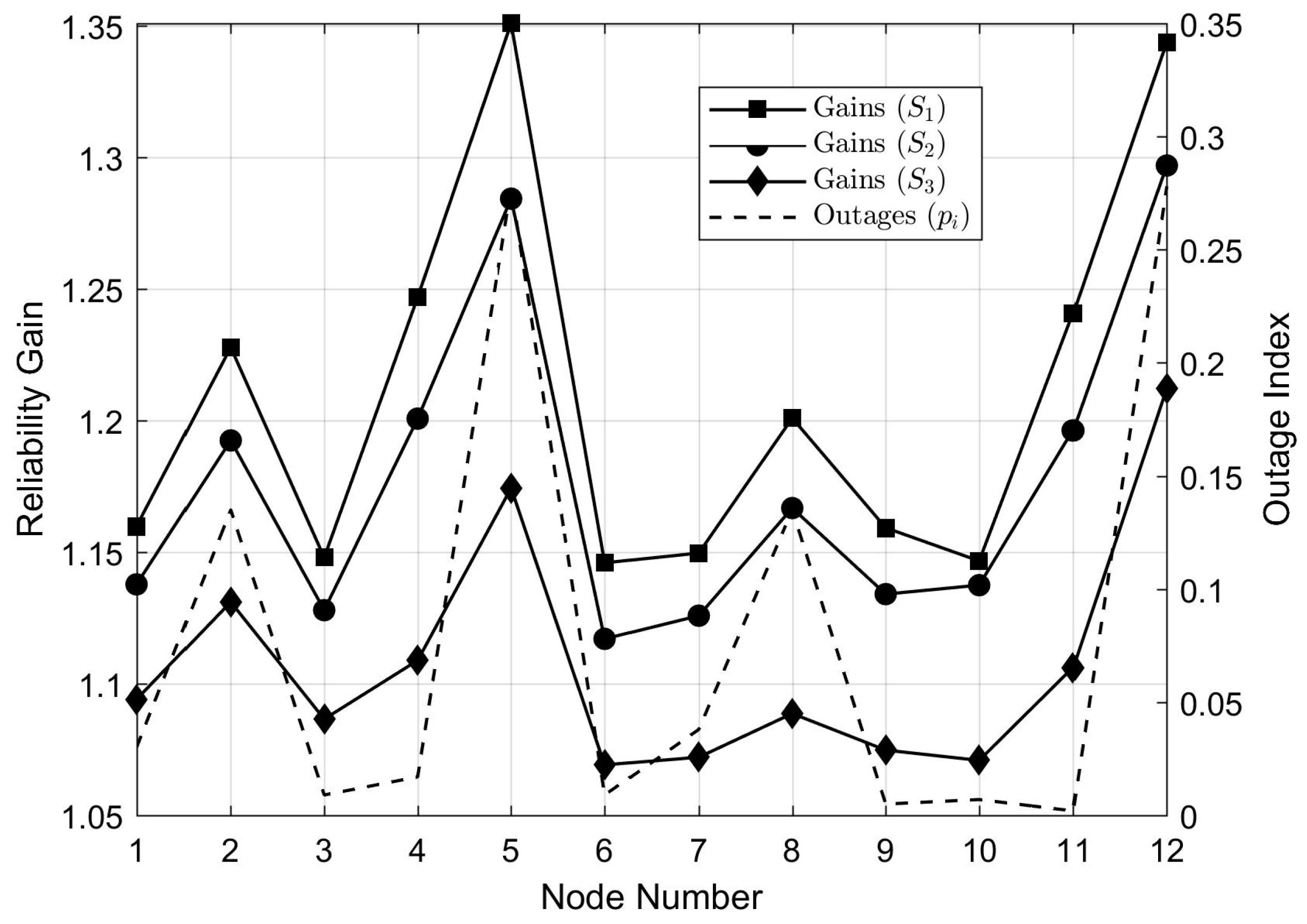
Considering that high values of DEC in a feeder imply frequent outages, it is clear that breakers protecting feeders with high DEC must be prioritized during communication link allocation. In this sense, we propose attributing link failure probabilities $p_{ij}=1-c_{ij}$ equal to the normalized value of the highest DEC associated with feeders protected by nodes $R_i$ and $R_j$.

We justify this heuristic in the following manner: for a greater value of $p_{ij}$ attributed to a certain link, the optimization algorithm will select solutions that possess redundancies around this link in order to maximize global reliability C. Therefore, redundancy allocation in the communication network will prioritize breakers that protect feeders with higher DEC values. In other words, the selected solutions will be the ones that attain greater communication reliability for breakers operating in faulty feeders.

Before indicating how to attribute the $c_{ij}$ to the network links, we note that there are two main types of breaker connections in power grids, namely grid and tie breakers [25]. Their difference resides in the natural state of operation and number of feeders to which they are connected: grid breakers are normally closed and protect one feeder, whereas tie breakers are normally open and connected between two feeders. Due to this difference, we shall propose slightly different heuristics for attributing $c_{ij}$ values in each case.

Let $DEC\left(F_i\right)$ denote the DEC of a feeder associated with node $R_i$. Considering that DEC is measured monthly, we have $0\mathrm{h}\le DEC\left(F_i\right)\le 720$ h. Given the network nodes and their associated feeder(s) with respective DEC value(s), we propose the following strategy for attributing reliabilities $c_{ij}$ to the network links:

• Normalize all $DEC\left(F_i\right)$ by $\Delta t=720$ h. The new values will be such that $DEC\left(F_i\right)\in [0,1]$;
• For every breaker $R_i$, verify if its type is a grid or tie. In the first case, define $p_i=DEC\left(F_i\right)$. Otherwise, define $p_i={\max }_{F_i}DEC\left(F_i\right)$.
• For every link from $R_i$ to $R_j$, attribute $p_{ij}=\max \left\{p_i,p_j\right\}$. Hence, $c_{ij}=1-\max \left\{p_i,p_j\right\}$.

The parameter $p_i$ associated with $R_i$ is equal to the DEC of the worst performing feeder to which this breaker is connected. Hence, $p_i$ can be interpreted as a measure of grid failure probability associated with $R_i$. For this attribution heuristic, it is clear that $\raisebox{1ex}{$\partial p_{ij}$}\!\left/ \!\raisebox{-1ex}{$\partial p_i$}\right.\ge 0$ and $\raisebox{1ex}{$\partial p_{ij}$}\!\left/ \!\raisebox{-1ex}{$\partial p_j$}\right.\ge 0$. Thus, the assigned $p_{ij}$ increase for greater node DEC values. This shows that nodes with unreliable feeders tend to decrease C, which makes the optimization process select network topologies that prioritize link redundancies between high-DEC nodes. The proposed strategy is summarized in Algorithm 2.

Algorithm 2: Computation of link reliabilities.

Input: $R_i$; $DEC\left(F_i\right)$, $1\le i\le n$.  Output: $c_{ij}$, $1\le i,j\le n$ 1: $DEC\left(F_i\right)\leftarrow \raisebox{1ex}{$DEC\left(F_i\right)$}\!\left/ \!\raisebox{-1ex}{$\Delta t$}\right.$, $\forall i$. 2: for$1\le i\le n$do 3:  if$R_i$ is grid-type then 4:   $p_i\leftarrow DEC\left(F_i\right)$. 5:  else 6:   $p_i\leftarrow {\max }_{F_i}DEC\left(F_i\right)$. 7:  end if 8: end for 9: $p_{ij}\leftarrow \max \left\{p_i,p_j\right\}$, $\forall i,j$. 10: $c_{ij}\leftarrow 1-p_{ij}$, $\forall i,j$. 11: return$c_{ij}$.

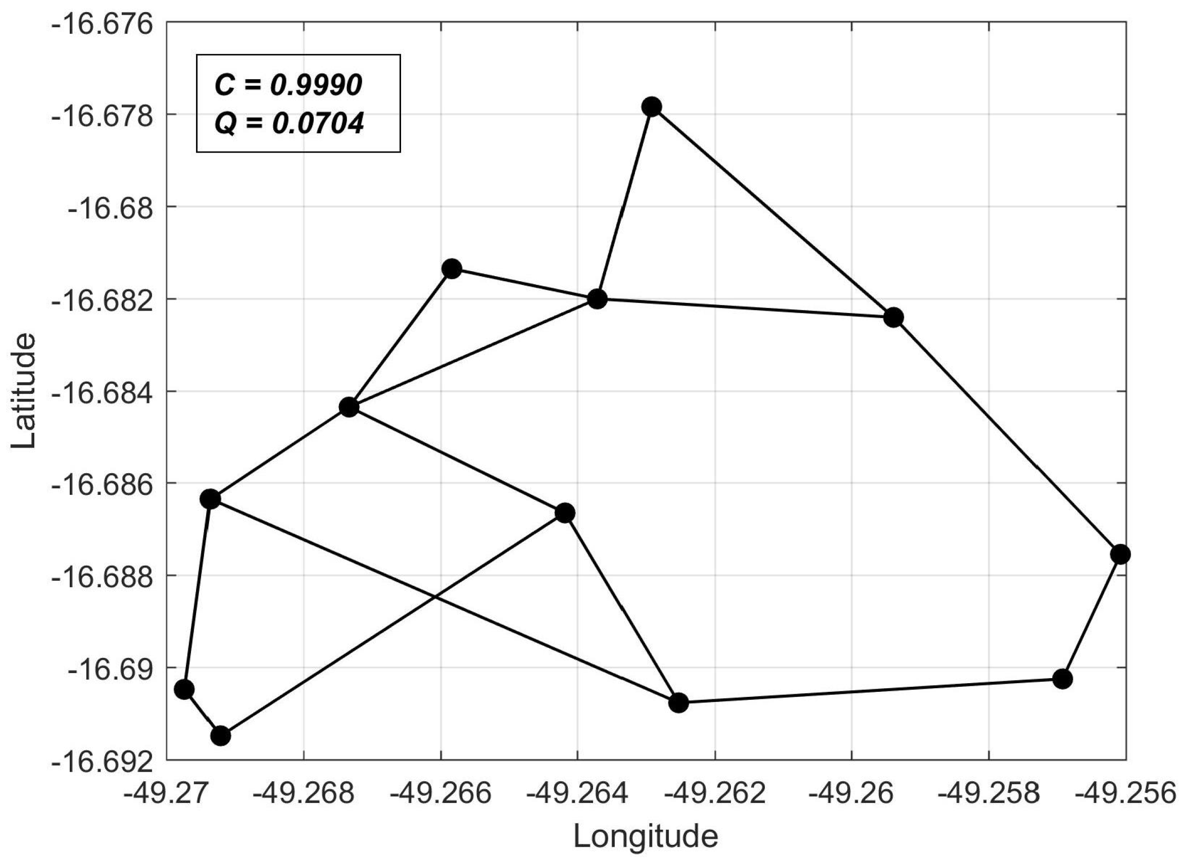
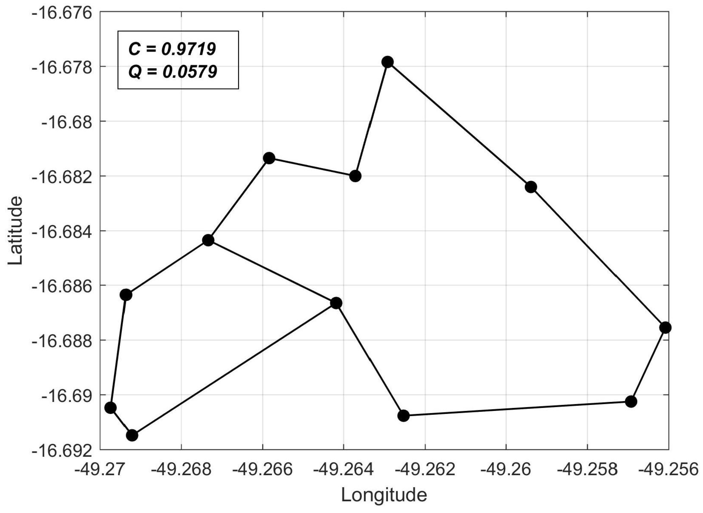
Considering that all $c_{ij}$ are attributed in a heuristic manner, we need a reference network topology against which we may compare C values computed for arbitrary networks. In this sense, we chose as a reference the shortest-perimeter ring topology, whose reliability we denote as $C_{ring}$. Thus, for any network topology, we can compute $\raisebox{1ex}{$C$}\!\left/ \!\raisebox{-1ex}{$C_{ring}$}\right.$ as a reliability measure, as will be shown in the computer experiments of Section 5.

3.3. Network Cost Computation

In the deployment of fiber optics links, cost is mainly associated with the required length of fiber needed. Hence, the network cost is a function of the distances between all node pairs that are connected by links. Let the node positions be identified in an arbitrary coordinate system by means of the set $R=\{(x_i,y_i),1\le i\le n\}$. Assuming the coordinates are known and denoting the distance between $R_i$ and $R_j$ by $d_{ij}$, we consider the euclidean distance $d_{ij}=\sqrt{{(x_i-x_j)}^2+{(y_i-y_j)}^2}$. Disregarding multiplicative factors for converting distance into monetary units, we compute the cost Q of a given topology as the sum of link lengths. Considering that optical links are implemented for bidirectional communication [26], we have $d_{ij}=d_{ji}$ and $a_{ij}=a_{ji}$. A factor $\raisebox{1ex}{$1$}\!\left/ \!\raisebox{-1ex}{$2$}\right.$ must be used to account for the bidirectional links. Hence, given the adjacency matrix A, the cost can be computed by:

$$Q=\frac{1}{2}\sum _{i=1}^n\sum _{j=1}^n{a}_{ij}{d}_{ij}=\sum _{i=1}^n\sum _{j=1}^i{a}_{ij}{d}_{ij}$$

(9)

We note that $a_{ii}=0$, as the existence of a self-connecting node is meaningless in the problem context. We now address handling of equivalent link costs in case the list $\mathsf{\Gamma }$ contains series or parallel links. If there are series links to be reduced, it is clear that the total distance is equal to the sum of individual link lengths. Hence, costs may simply be summed. For parallel links, the individual connections have approximately the same length. Therefore, the equivalent cost is equal to the individual link length multiplied by the total number of links.

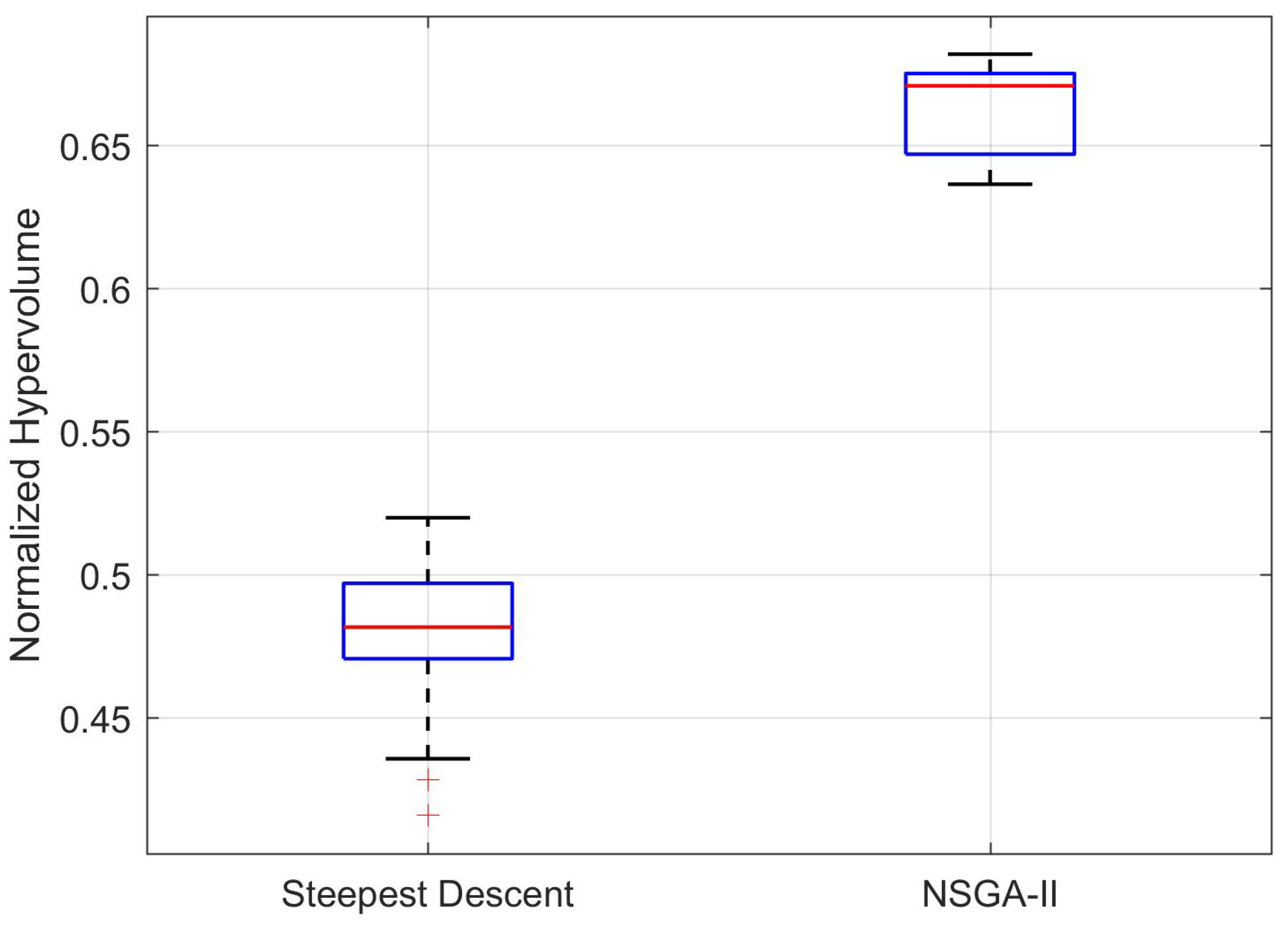
We shall use network cost Q as the second objective function to be optimized, alongside reliability C. Therefore, solutions obtained will represent different levels of compromise between these opposing factors. This approach is necessary in solving practical link allocation problems, since the amount of resources available for network deployment is limited.

3.4. Problem Constraints

Optimization problems usually present constraints in terms of the design variables and objective functions. In the link allocation problem, reasonable constraints would be maximum cost and minimum reliability values for all network solutions. However, this type of constraint disregards the connectivity of individual nodes.

For instance, a minimum value for C would not punish a network that achieves high reliability for all nodes, except for one that is left isolated. Likewise, a maximum Q value may cause links with good reliability that are never chosen due to their higher lengths. Based on these considerations, in what follows, we define alternative constraints that naturally limit cost and reliability, while still accounting for individual nodes.

We consider a physical constraint that can be given in terms of the design variables. Every  automated breaker has a maximum number of communication ports. Hence, there is a limit $n_e$ of links that can be connected to any network node. Supposing equal port limitation for all nodes, we address this constraint by defining a violation index [27] given by a step-form function:

$$d_i=(n_i-n_e)·u(n_i-n_e)=\left\{\begin{array}{ll}0,& \mathrm{if}{n}_i\le n_e;\\ n_i-n_e,& \mathrm{if}{n}_i>n_e\end{array}\right.$$

(10)

where $n_i$ is the number of links connected to node $R_i$. Analogously, we consider a minimum connectivity constraint $n_i\ge n_f$ for all nodes. This can be interpreted as ensuring any given node is supplied with sufficient link redundancies. The associated violation index is defined as:

$$d_i^{\prime }=(n_f-n_i)·u(n_f-n_i)$$

(11)

Depending on the type of optimization algorithm used to solve a problem, violation indexes can be implemented differently. For example, in gradient-based methods, they can be implemented as regularization terms in the objective function, whereas in genetic algorithms, they may be processed independently by means of binary tournament methods. The implementation of violation handling will be discussed in Section 4.

4. Choice of Optimization Method

The variables of the allocation problem are all $a_{ij}$ with $1\le i\le n$ and $j<i$. The restriction in the second index is due to bidirectional communication in optical links $(a_{ij}=a_{ji})$ and the absence of self-connected nodes $(a_{ii}=0)$. Hence, the total number of variables is $\left(\genfrac{}{}{0pt}{}{n}{2}\right)=\frac{n(n-1)}{2}$. Henceforth, we denote the set of all design variables by the vector $\mathit{a}$.

Practical optimization problems such as the one considered in this work are frequently intractable from the analytical point of view. This is due to a high number of variables and the involved form of the objective functions and their derivatives. In such cases, numerical solutions based on optimization algorithms must be used for solving the problem.

There are multiple classes of optimization algorithms, whose adequacy for application depends on problem representation, the domain, constraints, the ease of calculating objective function derivatives, and the computational complexity. In what follows, we will describe these characteristics for the allocation problem and establish the use of a genetic algorithm as most adequate.

The considered problem demands multi-objective optimization, since the compromise between cost and network reliability must be considered. Therefore, the objective functions to be optimized are C and Q, with the constraints established in Section 3. The number of design variables is $\left(\genfrac{}{}{0pt}{}{n}{2}\right)$, which may be high if the considered network has a large number of nodes. Problems with many variables can still be tractable if the objective functions are easy to compute. This is the case for Q, which is simply a linear combination of the variables. However, the computation of C is involved because all paths between every pair of nodes must be enumerated.

Given the computational cost of obtaining C and the large number of variables $a_{ij}$, second-order gradient-based optimization is impractical due to the large dimension of the Hessian matrix. Even if first-order optimization were considered, the burden imposed by the computation of derivatives would be excessive. To elaborate on this, let the reliability objective function be ${\mathcal{E}}_C\left(\mathit{a}\right)$. Computing a single derivative $\frac{\partial {\mathcal{E}}_C}{\partial a_{ij}}\left(\mathit{a}\right)$ would require enumeration of all paths for two different topologies, namely for $a_{ij}=1$ and $a_{ij}=0$. If $O\left(S\right)$ is the complexity of the enumeration algorithm, this procedure entails a complexity of $O\left(n^2\right)·O\left(S\right)$, as there are $\frac{n^2-n}{2}$ node pairs to consider. Finally, computing $\frac{\partial {\mathcal{E}}_C}{\partial \mathit{a}}\left(\mathit{a}\right)$ consists of repeating the procedure for all components of $\mathit{a}$. Hence, the complexity of a first-order method for computing C would be of order $O\left(n^4\right)·O\left(S\right)$.

Furthermore, in gradient-based methods, ${\mathcal{E}}_C\left(\mathit{a}\right)$ should contain a regularization term for punishing unfeasible solutions. In this sense, we would have ${\mathcal{E}}_C\left(\mathit{a}\right)={\mathcal{E}}_{C_o}\left(\mathit{a}\right)+\lambda {\mathcal{R}}_C\left(\mathit{a}\right)$, where ${\mathcal{E}}_{C_o}$ is a function of C, ${\mathcal{R}}_C\left(\mathit{a}\right)$ is the regularization term, and $\lambda$ is the weight given to this term. The choice of $\lambda$ is not trivial and may be problematic, since its optimal value may vary for different instances of the optimization problem.

We now argue that genetic algorithms can be used for optimization without the difficulties previously presented. Since this type of algorithm consists of evaluating the fitness of stochastically-generated solutions, the problem of computing derivatives is immediately eliminated. Furthermore, the constraint handling procedures are usually independent of objective function evaluation, making weight parameters such as $\lambda$ unnecessary. Since derivatives do not need to be computed, reliability evaluation will present only $O\left(n^2\right)·O\left(S\right)$ complexity.

The allocation problem variables are naturally coded as a binary digit string given by $\mathit{a}$, since all variables are such that $a_{ij}\in \left\{0,1\right\}$. This type of representation is required for applying the genetic algorithm operators, such as mutation and crossover, to the solution ensemble. The absence of a need to convert the problem data into an abstract binary representation shows it is naturally fit for the data representation used in genetic algorithms.

As a final argument for the use of genetic algorithms, we shall establish a loose lower bound for the number of feasible solutions that is proportional to $\left[\right(n-1)!]$. The large problem domain is another reason for considering genetic algorithms. We make the following proposition:

Theorem 1.

The number $N_s$ of feasible solutions for the problem:

• ${\mathit{minimize}}_{\mathit{a}}Q\left(\mathit{a}\right)$;
• ${\mathit{maximize}}_{\mathit{a}}C\left(\mathit{a}\right)$;
• $\mathit{subject}\mathit{to}{n}_i\le n_e\mathit{and}{n}_i\ge n_f,i=1,2,\dots ,n$

has a lower bound given by $N_s\ge K_s·(n-1)!$, where $K_s<[n·(n_e-n_f)+1]$ and $K_s\in {\mathbb{N}}^{*}$.

Proof of Theorem 1.

Let $N_s\left(k\right)$ denote the number of solutions that have ${\sum }_{i=1}^n{n}_i=k$, with $n·n_f\le k\le n_{max}$, where $n_{max}<n·n_e$. Clearly, $N_s={\sum }_{k=n·n_f}^{n_{max}}{N}_s\left(k\right)$. Now, we consider a particular case with the most severe node connection restrictions, namely $n_e=n_f=2$. We disregard the case of nodes with only one connection because this would imply topologies with isolated node pairs.

For the particular case chosen, denote the number of possible solutions by $N_s^{*}$. Since all nodes are forced to have two connections, the amount of solutions is the number of node circular permutations, $N_s^{*}=[(n-1)!]$. Returning to the general problem, it is clear that we have $N_s\left(k\right)\ge N_s^{*}$ for every k. Therefore, we have:

$$N_s\ge \sum _{k=n·n_f}^{n_{max}}{N}_s^{*}=(n_{max}-n·n_f+1)·(n-1)!=K_s·(n-1)!$$

(12)

Since $n_{max}\ge n·n_f$, we have $K_s\in {\mathbb{N}}^{*}$. Furthermore, using the fact that $n_{max}<n·n_e$, we get $K_s<[n·(n_e-n_f)+1]$, and the proof is concluded. □

The lower bound obtained is very loose, since for large k, the number of possible solutions tends to be much higher than that for $k=2$. However, in spite of being conservative, the obtained bound grows with $(n-1)!$, which shows that the feasible domain is very large. Coupled with the previous discussions, this fact makes a strong case for using genetic algorithms.

4.1. Implementing the Optimization Method with NSGA-II

We opted for implementing the optimization routine with the non-dominated sorting genetic algorithm II (NSGA-II) [27]. The main reasons for selecting this genetic algorithm are its satisfactory computational complexity and lack of tuning parameters. Furthermore, when compared to NSGA-III, it has similar performance for two-objective problems and a simpler implementation of the solution crowding operator [28]. For M objectives and N individuals per generation, the complexity of NSGA-II is $O\left(M{N}^2\right)$ per generation. The algorithm manages constraints separately from objective function evaluation, which means a weight parameter for constraint violation is not needed. The ranking of solutions is done on a binary tournament basis, in which the criteria are solution fitness and constraint violations.

A weakness of many multi-objective genetic algorithms is the fact that they require a prespecified parameter $\sigma$ for controlling the variety of obtained solutions. Ideally, the Pareto front should be as diverse as possible. In order to obtain good results, trial and error with various $\sigma$ values may be necessary. Furthermore, the optimal parameter value is prone to change for different problem instances. This difficulty is surpassed in NSGA-II by using a crowding operator that naturally selects the most diverse solutions: if two solutions are tied in the ranking process, the solution most distant from the rest is selected by the operator.

Aside from the ranking and crowding operators, which were implemented as given in Deb et al. [27], we used mutation and crossover operators for population evolution. We opted for uniform crossover and bitwise mutation with probabilities $p_c=0.7$ and $p_m=0.03$, respectively. Using uniform crossover in this problem is more reasonable than k-point crossover, since exchanging large bit substrings of two solution vectors is very likely to generate network solutions with isolated nodes. The initial population was generated randomly with a uniform distribution, and the evolutionary process was set to run for $G=30$ generations with $N=100$ individuals each.

All algorithm parameters were selected by means of preliminary manual tests. Values of N and G were gradually increased until their variation did not significantly contribute to solution front variety and convergence, respectively. For selecting mutation and crossover probabilities, we used the standard metaheuristic of starting with low values of $p_m$ and high values of $p_c$. This procedure avoids stagnation and high degrees of randomness in the evolutionary process [29]. The selected values are those for which the best results were obtained in the preliminary tests.

The NSGA-II algorithm is designed for minimizing all of its objective functions. In the considered allocation problem, cost must be minimized and reliability maximized. In order to adapt the reliability objective to NSGA-II, we ran the optimization in Q and $-C$.

The optimization algorithm implementation with NSGA-II is described in Algorithm 3. We denote by $\mathsf{\Omega }$ the set of all lists $\mathsf{\Gamma }$ that represent possible solutions. Furthermore, G and N are the numbers of generations and individuals per generation, respectively.

Algorithm 3: Network optimization via NSGA-II.

Input: $R_i$, $1\le i\le n$; G; N; $p_m$; $p_c$.  Output: Pareto front. 1: Generate a random family of N lists ${\mathsf{\Gamma }}_i^{\left(0\right)}\subset \mathsf{\Omega }$, $i=1,2,\dots ,N$. 2: for$1\le j\le G$do 3:  for $1\le i\le N$ do 4:   Compute Equation (9). 5:   Execute Algorithm 1. 6:   return $(Q_i,-C_i)$. 7:  end for 8:  Execute NSGA-II over objectives Q and $(-C)$. 9:  return New family of N lists ${\mathsf{\Gamma }}_i^{\left(j\right)}\subset \mathsf{\Omega }$, $i=1,2,\dots ,N$. 10: end for 11: return Pareto front.

4.2. Alternative Implementation with Objective Priority

An important aspect in practical optimization problems is the attribution of priority levels to objective functions, which is not covered by NSGA-II. However, the algorithm compensates for this by supplying as output a Pareto front containing solutions with different degrees of optimality for the objective functions. However, from the perspective of a decision maker, it may be desirable to have a priority mechanism that yields a single solution. In the problem context, this corresponds to the utility having a previously established reliability-cost ratio.

In this sense, we propose a simple alternative implementation that can be substituted for the standard NSGA-II when desired. It consists of making a linear combination of Q and C and using the same routine as in Algorithm 3 for optimizing this linear combination in a mono-objective fashion. In other terms, the objective function is given by:

$$Z=r_Q·\frac{Q}{Q_{max}}-r_C·C,$$

(13)

where $r_C>0$ and $r_Q>0$ are, respectively, weights associated with the original objective functions C and Q; these weights are such that $r_C+r_Q=1$. Cost is normalized by the maximum cost solution $Q_{max}$ so that both objectives Q and C belong to the interval $[0,1]$, which is needed for the correct weight attribution [30].

If multiple objective functions are linearly combined with weights that sum to one, the mono-objective optimization will converge to a solution belonging to the Pareto front that would be obtained via multi-objective optimization [30]. In this sense, the use of weights establishes a mechanism for automatically selecting desired regions of the solution space. This is of interest for a decision maker that possesses previous information concerning the desired solution, since the search is already directed towards the most adequate solution of the Pareto front.

4.3. Computational Complexity

Now that the optimization method is established, we derive its computational complexity. We initially consider the complexity of path enumeration, namely that of Yen’s algorithm. This algorithm has a complexity that depends on the auxiliary method used for obtaining the shortest path [24]. Due to its simplicity, we used Dijkstra’s algorithm as the auxiliary method. In this case, the search complexity is $O\left(K{n}^3\right)$ [31], where n is the number of nodes and K is the maximum number of paths to be enumerated in each iteration.

We previously established a complexity of $O\left(n^2\right)·O\left(S\right)$ for evaluating the reliability of a single solution. Substituting $O\left(S\right)=O\left(K{n}^3\right)$, we get a complexity $O\left(K{n}^5\right)$. From Equation (9), the computation of a solution cost is seen to be $O\left(n^2\right)$. Considering that the reliability and cost of a solution are computed sequentially, we have a complexity $O(K{n}^5+n^2)=O\left(K{n}^5\right)$ per solution. The complexity of NSGA-II for processing one population is $O\left(M{N}^2\right)$. Since each solution has an evaluation complexity of $O\left(K{n}^5\right)$, we get a total complexity of $O\left(KM{N}^2{n}^5\right)$ per generation.

Reasoning in a similar manner for first-order gradient algorithms, we obtain a complexity $O\left(K{n}^7\right)$ for computing each solution. If the algorithm was of a stochastic gradient-descent type, it would require multiple iterations and increase the complexity even further. Hence, using NSGA-II is advantageous in terms of complexity at least to an order of $O\left(n^2\right)$ per solution.

It is clear that the complexity of the proposed method strongly depends on n. On the other hand, it advantageously has polynomial behavior. It can be seen that a good choice of K can help decrease complexity. However, this parameter must be kept sufficiently high in order to guarantee low approximation errors during reliability computations.

5. Case Study

The proposed heuristic and optimization method were applied to a practical problem considered in a research project by the local distribution utility (CELG-D) for automating a group of breakers in its grid. The considered scenario consisted of the allocation of optical links for $n=12$ recently installed grid breakers with physical constraints $n_f=2$, $n_e=4$.

In

Table 1. Coordinates and $p_i$ of network nodes.

Node	Latitude $\left(\mathit{x}\right)$	Longitude $\left(\mathit{y}\right)$	${\mathit{p}}_{\mathit{i}}={\mathbf{max}}_{{\mathit{F}}_{\mathit{i}}}\mathit{DEC}\left({\mathit{F}}_{\mathit{i}}\right)$
1	−49.269734	−16.690475	0.030
2	−49.269209	−16.691483	0.135
3	−49.269359	−16.686351	0.009
4	−49.256929	−16.690250	0.017
5	−49.262528	−16.690768	0.278
6	−49.267333	−16.684356	0.009
7	−49.263707	−16.682012	0.038
8	−49.259385	−16.682414	0.135
9	−49.262919	−16.677848	0.005
10	−49.265832	−16.681361	0.007
11	−49.256081	−16.687550	0.002
12	−49.264181	−16.686651	0.278

, we present the coordinates of all nodes in the coordinate system adopted by the utility. The $p_i$ parameters computed for each node by using Algorithm 2 are also given. The computation was based on DEC data in the utility database. The positions of all breakers are illustrated in Figure 1, where we also display the reference ring network topology.

We then applied Algorithm 3 to the obtained $p_i$ for attributing all link reliabilities $c_{ij}$. These values are given in the matrix $C_o={\left[c_{ij}\right]}_{12\times 12}$ as follows:

$$C_o=\left({\displaystyle \begin{array}{cccccccccccc}0& 0.9175& 0.9805& 0.9765& 0.8460& 0.9805& 0.9660& 0.9175& 0.9825& 0.9815& 0.9775& 0.8460\\ 0.9175& 0& 0.9280& 0.9240& 0.7935& 0.9280& 0.9135& 0.8650& 0.9300& 0.9290& 0.9250& 0.7935\\ 0.9805& 0.9280& 0& 0.9870& 0.8565& 0.9910& 0.9765& 0.9280& 0.9930& 0.9920& 0.9880& 0.8565\\ 0.9765& 0.9240& 0.9870& 0& 0.8525& 0.9870& 0.9725& 0.9240& 0.9890& 0.9880& 0.9840& 0.8525\\ 0.8460& 0.7935& 0.8565& 0.8525& 0& 0.8565& 0.8420& 0.7935& 0.8585& 0.8575& 0.8535& 0.7220\\ 0.9805& 0.9280& 0.9910& 0.9870& 0.8565& 0& 0.9765& 0.9280& 0.9930& 0.9920& 0.9880& 0.8565\\ 0.9660& 0.9135& 0.9765& 0.9725& 0.8420& 0.9765& 0& 0.9135& 0.9785& 0.9775& 0.9735& 0.8420\\ 0.9175& 0.8650& 0.9280& 0.9240& 0.7935& 0.9280& 0.9135& 0& 0.9300& 0.9290& 0.9250& 0.7935\\ 0.9825& 0.9300& 0.9930& 0.9890& 0.8585& 0.9930& 0.9785& 0.9300& 0& 0.9940& 0.9900& 0.8585\\ 0.9815& 0.9290& 0.9920& 0.9880& 0.8575& 0.9920& 0.9775& 0.9290& 0.9940& 0& 0.9890& 0.8575\\ 0.9775& 0.9250& 0.9880& 0.9840& 0.8535& 0.9880& 0.9735& 0.9250& 0.9900& 0.9890& 0& 0.8535\\ 0.8460& 0.7935& 0.8565& 0.8525& 0.7220& 0.8565& 0.8420& 0.7935& 0.8585& 0.8575& 0.8535& 0\end{array}}\right)$$

Given the $c_{ij}$ and node coordinates, we first computed cost $Q_{ring}$ and reliability $C_{ring}$ for the ring network (Figure 1). As previously discussed, the reliability $C_{ring}$ is used as a reference for comparison with the obtained solutions. It is also of interest to compare solution costs to $Q_{ring}$ because this topology is considered low cost while attaining good reliability. The obtained values were $Q_{ring}=0.0497$ and $C_{ring}=0.8283$. Considering the good compromise between cost and reliability achieved by ring networks, it is expected that the Pareto front should be in the neighborhood of the reference ring solution.

The proposed optimization algorithm was run for $G=30$ generations with $N=100$ individuals each, with the value $K=100$ for Yen’s algorithm maximum path number parameter. At first, standard multi-objective optimization was considered. In a second run of the algorithm, we used the alternative implementation with objective priority, testing for different weights $r_V$ and $r_Q$. The obtained results are described in what follows.

5.1. Weightless Optimization

Initially, regular multi-objective optimization was applied. The obtained Pareto front is depicted in Figure 2. In Figure 3, Figure 4 and Figure 5, we present the network topologies, costs, and reliabilities of three solutions sampled from the Pareto front (denoted $S_1$, $S_2$, and $S_3$ in Figure 2).

The sampled solutions allow us to visualize the solution behavior along the Pareto front. It can be seen that, the closer to the Q-axis a solution is, the higher its reliability and cost are. The relative reliability gains $\raisebox{1ex}{$C_i$}\!\left/ \!\raisebox{-1ex}{$C_i^{\left(ring\right)}$}\right.$ for each node, together with the overall gain $\raisebox{1ex}{$C$}\!\left/ \!\raisebox{-1ex}{$C^{\left(ring\right)}$}\right.$, are given in

Table 2. Reliability gains (weightless optimization).

Node	$\frac{{\mathit{C}}_{\mathit{i}}}{{\mathit{C}}_{\mathit{i}}^{\left(\mathit{ring}\right)}}\left({\mathit{S}}_3\right)$	$\frac{{\mathit{C}}_{\mathit{i}}}{{\mathit{C}}_{\mathit{i}}^{\left(\mathit{ring}\right)}}\left({\mathit{S}}_2\right)$	$\frac{{\mathit{C}}_{\mathit{i}}}{{\mathit{C}}_{\mathit{i}}^{\left(\mathit{ring}\right)}}\left({\mathit{S}}_1\right)$
1	1.0941	1.1378	1.1599
2	1.1311	1.1925	1.2279
3	1.0866	1.1280	1.1480
4	1.1089	1.2008	1.2469
5	1.1744	1.2844	1.3511
6	1.0692	1.1171	1.1460
7	1.0721	1.1259	1.1497
8	1.0887	1.1668	1.2010
9	1.0748	1.1341	1.1593
10	1.0709	1.1375	1.1467
11	1.1061	1.1963	1.2407
12	1.2123	1.2970	1.3439
Overall	1.1053	1.1733	1.2061

for the sampled solutions $S_1,S_2$, and $S_3$.

5.2. Optimization with Weight Assignment

The algorithm with objective priority was run for the weight values shown in

Table 3. Chosen weight pairs.

Pair	${\mathit{r}}_{\mathit{C}}$	${\mathit{r}}_{\mathit{Q}}$
$P_1$	$0.8$	$0.2$
$P_2$	$0.5$	$0.5$
$P_3$	$0.2$	$0.8$

. The solutions obtained for each $(r_Q,r_C)$ pair, with their respective reliability and cost values, are given in Figure 6, Figure 7 and Figure 8. The reliability gains for each solution are given in

Table 4. Relative gains (weight optimization).

Node	$\frac{{\mathit{C}}_{\mathit{i}}}{{\mathit{C}}_{\mathit{i}}^{\left(\mathit{ring}\right)}}\left({\mathit{P}}_3\right)$	$\frac{{\mathit{C}}_{\mathit{i}}}{{\mathit{C}}_{\mathit{i}}^{\left(\mathit{ring}\right)}}\left({\mathit{P}}_2\right)$	$\frac{{\mathit{C}}_{\mathit{i}}}{{\mathit{C}}_{\mathit{i}}^{\left(\mathit{ring}\right)}}\left({\mathit{P}}_1\right)$
1	1.0000	1.1388	1.1541
2	1.0000	1.1924	1.2214
3	1.0000	1.1295	1.1453
4	1.0000	1.2071	1.2370
5	1.0000	1.2858	1.3380
6	1.0000	1.1197	1.1382
7	1.0000	1.1425	1.1425
8	1.0000	1.1735	1.1946
9	1.0000	1.1379	1.1565
10	1.0000	1.1216	1.1392
11	1.0000	1.2027	1.2312
12	1.0000	1.2958	1.3333
Overall	1.0000	1.1757	1.1987

. The Pareto front points corresponding to the obtained solutions are labeled, in Figure 2, as $P_1$, $P_2$, and $P_3$. As expected, all solutions belong to the front obtained via multi-objective optimization.

5.3. Analysis of the Results

The results in Table 2 and Table 4 show greater reliability gains in nodes associated with higher DEC indexes. In this sense, the heuristic for allocating greater network resources to the high-DEC nodes is validated. To further illustrate this, in Figure 9, we plot node reliability gains together with DEC values for the weightless multi-objective optimization results.

The results depicted in Figure 9 show that link allocation was such that reliability gains were higher for nodes with worse associated outage values. The only exception to this relation is the set of Nodes 9–11. However, this behavior can be explained by the fact that, in spite of having lower outage values than Node 10, Nodes 9 and 11 had neighboring nodes (8 and 12) with significantly higher outage values. It is also important to note that the slopes of the gain curves had the same general behavior as the slope of the outage curve, which further suggests greater network resource allocation for worse performing feeders.

We note that, despite a relatively high N value, the obtained Pareto front does not have a very large amount of solutions. This can be explained by the binary domain of $a_{ij}$, which makes a small number of solutions maintain dominance throughout the evolution process of NSGA-II. Furthermore, the constraints $n_f\le n\le n_e$ reduce the number of feasible solutions.

As shown in Figure 2, one of the obtained solutions is the ring network itself. This is also a reasonable result: the ring topology has the least cost among all solutions that provide the minimum required connectivity between grid breakers. Therefore, it always maintains dominance with respect to other solutions in terms of the Q objective function.

The weight-assignment method converged to reasonable regions of the solution space for all weight pairs. Furthermore, convergence to a point belonging to the Pareto front was always verified, which is in accordance with the theoretical considerations. In particular, the attribution of high priority to cost correctly resulted in convergence to the ring topology.

5.4. Reliability Estimation Performance

As previously discussed, the parameter K must be adequately chosen for preventing large errors in reliability estimation. In order to validate the estimations of this case study in terms of error and to illustrate dependence on K, we consider a test scenario in which estimation is prone to much higher errors than in the previously considered real case. For this scenario, we consider the case in which all links have equal and low-valued $c_{ij}$.

If the individual reliabilities $c_{ij}$ are equal, the reliability of any path $L_k$ does not have dominant terms, as can be seen in Equation (1). This means that excluding paths from the reliability computation will cause more significant losses in accuracy. In addition, since the $c_{ij}$ are low-valued, convergence of the external product series in Equation (1) is slow and more terms are required in order to compute $C_{ij}$ precisely.

In the test case, we used the same system with $n=12$ nodes, but with path reliabilities $c_{ij}=0.1$; it is clear that this value is much lower than that found in the real system. Thus, reliability estimation is more demanding. Fifty topologies were randomly generated with a uniform distribution, and their reliabilities were estimated by using all values $K=10·i$, $i=1,2,\dots ,20$.

All computed reliability values were normalized in relation to the ones obtained with the parameter $K=10$. Denoting by $C^{\left(i\right)}\left(K\right)$ the normalized value obtained for the ith topology, we computed the ensemble average $C^{\left(avg\right)}\left(K\right)=\frac{1}{50}·{\sum }_{i=1}^{50}{C}^{\left(i\right)}\left(K\right)$, $\forall K$. We also computed the increments $\Delta C^{\left(avg\right)}\left(K\right)=C^{\left(avg\right)}(K+1)-C^{\left(avg\right)}\left(K\right)$ in order to evaluate the convergence of the ensemble average of estimated reliabilities for growing K. The results are given in Figure 10.

The results show that estimation error is rapidly reduced for increasing K, which causes rapid convergence of the estimated reliability. As an example, the highlighted point in Figure 10 shows that, for $K>40$, the ensemble average $C^{\left(avg\right)}\left(K\right)$ increases less than $0.01$ for an additional path enumerated with Yen’s algorithm. Considering these results and the fact that the selected test case is more demanding in terms of reliability computation than the optimization problem, our choice of $K=100$ in the case study is justified.

We note that this type of test case can be used because the convergence of $C^{\left(avg\right)}\left(K\right)$ implies that the estimation error $ϵ\left(K\right)=C^{\left(avg\right)}\left(K\right)-C^{\left(avg\right)}$ converges to zero, where $C^{\left(avg\right)}$ is the real reliability average. In fact, for growing K, the number of ignored paths decreases, and due to the enumeration of paths with decreasing reliabilities in Yen‘s algorithm, the increments $C^{\left(avg\right)}\left(K\right)$ are decreasing. Finally, since ${\beta }_{ij}$ is finite, it is clear that $ϵ\left(K\right)=0$ for $K\ge {\max }_{(i,j)}{\beta }_{ij}$.

5.5. Performance Comparison with the Steepest-Descent Gradient Method

In Section 4, we compared the proposed optimization with gradient-based methods in terms of theoretical computational complexity. To provide a concrete comparison, we also apply a local search-type algorithm to solve the allocation problem. We also adopted this procedure because, aside from complexity, it is important to test the capacity of different methods to avoid local minima and converging to high-quality solutions.

The chosen algorithm was the standard discrete-domain steepest descent search [32], which we now briefly describe. Given an arbitrary solution vector $\mathit{a}$, we define its neighborhood $\mathcal{N}\left(\mathit{a}\right)$ as the set of all other solutions ${\mathit{a}}_{\mathit{i}}$ such that $|\mathit{a}-{\mathit{a}}_{\mathit{i}}|=1$. We then define the objective function $f\left(\mathit{a}\right)$ to be minimized and randomly choose an initial solution ${\mathit{a}}_{\mathit{o}}$. The first step consists of evaluating the objective for all vectors in $\mathcal{N}\left({\mathit{a}}_{\mathit{o}}\right)$ and returning the vector ${\mathit{a}}^{\prime }={\mathrm{argmin}}_{[\mathit{a}\in \mathcal{N}\left({\mathit{a}}_{\mathit{o}}\right)]}f\left(\mathit{a}\right)$. This vector is now treated as the current solution $\mathit{a}$, and the procedure is iterated by minimizing the objective function in $\mathcal{N}\left(\mathit{a}\right)$. The algorithm may be stopped for a given number of iterations or according to a specified convergence criterion.

For this approach, we formulate the allocation problem with a single objective function that encompasses reliability, cost, and constraints. Considering that the algorithm is mono-objective and has no priority mechanisms, in each algorithm run, we randomly chose weights for Q and C in order to obtain more varied solutions. Hence, we used the following objective function:

$$f\left(\mathit{a}\right)=r_Q·\frac{Q\left(\mathit{a}\right)}{Q_{max}}-r_C·C\left(\mathit{a}\right)+\sum _{i=1}^n(d_i+d_i^{\prime }),$$

(14)

where $r_Q\sim U(0,1)$ and $r_C=1-r_Q$, with the weights being generated in every algorithm run. The last term is the regularization term and is equal to the sum of violation constraints. We attributed a weight $\lambda =1$ to this term, in order to harshly punish unfeasible solutions.

The optimization was set to 30 steepest-descent runs, with 100 iterations in each run. These numbers were selected to match respectively the generation and population numbers used with NSGA-II.

In order to compare the optimization approaches statistically, each one was run a total of 40 times for the study case. In what follows, we compare the results in terms of time performance, solution dominance, and statistical properties of the obtained hypervolume indicators.

5.5.1. Comparison between Least-Dominated Solution Fronts

As a preliminary means of comparison, among the 40 solution fronts obtained for each optimization method, we selected the one with the smallest number of dominated solutions with respect to the remaining fronts. In Figure 11, we compare the selected least-dominated fronts.

Furthermore, we compare the selected fronts in terms of execution time per solution. Let $t_{NSGA}\left(i\right)$ denote the average evaluation time of all solutions belonging to generation i. Furthermore, define $t\left(i\right)$ as the time required for computing the ith solution of the steepest-descent method. In Figure 12, we plot the ratio $\raisebox{1ex}{$t\left(i\right)$}\!\left/ \!\raisebox{-1ex}{$t_{NSGA}\left(i\right)$}\right.$ for all $i=1,2,\dots ,G$, where $G=30$ is the total generation number.

The comparisons show that steepest descent optimization yielded a worse solution front than the one obtained with NSGA-II. In fact, Figure 11 shows that all solutions found with the steepest descent were dominated by the NSGA-II solutions with respect to both objectives.

Figure 12 shows that computational time for the steepest descent method was significantly higher per solution than that of NSGA-II. It is interesting to note that the deduction (from Section 4) that complexity per solution of steepest descent is $O\left(n^2\right)$ greater than that of NSGA-II was validated by the results. Considering that each generation of NSGA-II has $N=100$ individuals, the results showed that the execution time for one generation was in the same order of magnitude of the execution time for a single steepest-descent solution. Hence, NSGA-II had a significant advantage of providing a greater variety of solutions than steepest descent for a fixed time interval.

5.5.2. Statistical Comparison

In spite of the conclusions that may be drawn from comparisons between solution front instances, statistical analysis of optimization methods must be carried out to evaluate their capabilities to provide high quality solution fronts consistently. In order to compare the considered algorithms, we computed the hypervolume indicator and its main statistical indexes for each set of 40 solution fronts.

The hypervolume of a solution front is a measure of its coverage of the solution space. Hence, it is an effective parameter for evaluating solution front quality. The computation of the hypervolume requires the choice of a reference point in the solution space. A heuristic criterion for selecting a reference point that attributes hypervolume values in proportion to solution front quality is given by [33]:

$$r_1=r_2\ge 1+\frac{1}{N_p-1}$$

(15)

where $\mathit{R}(r_1,r_2)$ is the reference point in the normalized solution space coordinates and $N_p$ is the number of solutions in the Pareto front. Considering that $N_p\le N=30$, we adopt a conservative value $N_p=10$ in Equation (15), which yields a lower bound equal to $1.11$. Hence, we choose the normalized reference point $\mathit{R}(1.2,1.2)$ for computing front hypervolumes. The solution space cost and reliability values were normalized by their respective maximum values among all obtained solution fronts.

The following summary statistics of normalized hypervolume were computed: minimum value, maximum value, average, and standard deviation. The comparison of hypervolume statistics for both algorithms is given in

Table 5. Statistics of the normalized hypervolume.

Parameter	NSGA-II	Steepest Descent
Average	$0.6617$	$0.4795$
Standard Deviation	$0.0156$	$0.0267$
Maximum Value	$0.6817$	$0.5197$
Minimum Value	$0.6363$	$0.4156$

, and the boxplot of the corresponding data is given in Figure 13.

In order to further compare the time performance of the algorithms, we also evaluated the execution time per solution for all solution fronts. The corresponding summary statistics and boxplot for this parameter are given in

Table 6. Statistics of execution time per solution (in seconds).

Parameter	NSGA-II	Steepest Descent
Average	$3.5389$	$183.7337$
Standard Deviation	$2.8003$	$6.4778$
Maximum Value	$10.6169$	$194.4681$
Minimum Value	$1.3776$	$159.0220$

and Figure 14, respectively.

The statistical results suggest that the proposed NSGA-II approach yields significantly better time performance and solution front quality than the steepest descent algorithm. The average front hypervolume for NSGA-II was $38\%$ greater in relation to the one obtained with steepest descent, whereas the ratio between average execution time for NSGA-II and steepest descent was $1.93\%$. As similarly noted in Section 5.5.1, the results also support the conclusion that time complexity is smaller by an order $O\left(n^2\right)$ for the proposed method.

6. Conclusions

In this work, we proposed a new reliability-based heuristic for optimizing optical link deployment in a network for connecting automated power grid breakers. The heuristic consisted of attributing link reliability values as functions of grid outage indexes. The proposed heuristic was implemented with an approximate reliability computation method for reducing complexity. Multi-objective optimization considering reliability and network cost was then carried out with NSGA-II. The choice of a genetic algorithm was justified by the problems that would be encountered by using gradient-descent methods, such as computational complexity, and involved evaluation of reliability derivatives.

The method was validated with a 12-node case study using real information from the database of the local distribution utility. The results showed that the proposed algorithm, aside from optimizing the objective functions, allocated more network resources to nodes located in feeders with higher outage indexes, as intended. Furthermore, it was shown that the performance of the proposed algorithm was superior in comparison to first-order gradient search, both in terms of quality (evaluated by dominance and hypervolume indicator) of the obtained solution fronts and computation time per solution.

It was shown that the proposed approach had a computational complexity that was polynomial in the number of network nodes. Hence, we believe the proposed method has good scalability for application in problems with node numbers of higher magnitudes.

The main contribution of this work consists of the proposal and validation of a novel procedure for optimizing the allocation of communication links associated with automated power grid breakers. The presented multi-objective approach, coupled with the proposed heuristic, enables the optimization of network topology in terms of cost and reliability while prioritizing reliability gains of breakers associated with high-outage feeders. Furthermore, the output of a Pareto front is useful in aiding the decision-making process by the stakeholders in real applications.

We believe the proposed optimization method is of interest because it simultaneously considers power grid contingency indexes and network cost for optimizing the link allocation. To the best of our knowledge, no previous work has addressed the optimization of communication links between elements in the power grid from this point of view.

References

1. National Agency of Electrical Energy (ANEEL). Module 8 of the Procedures for Distribution of Electrical Energy in the National Electric System (PRODIST), 8th ed.; National Agency of Electrical Energy (ANEEL): Sao Paulo, Brazil, 2018.
2. Billinton, R.; Allan, R. Reliability Evaluation of Engineering Systems: Concepts and Techniques; Springer: New York, NY, USA, 2013. [Google Scholar]
3. Blackburn, J.; Domin, T. Protective Relaying: Principles and Applications, 4th ed.; Power Engineering (Willis) Series; Taylor & Francis: New York, NY, USA, 2014. [Google Scholar]
4. Schacht, D.; Lehmann, D.; Kalisch, L.; Vennegeerts, H.; Krahl, S.; Moser, A. Effects of configuration options on reliability in smart grids. CIRED-Open Access Proc. J 2017, 2017, 2250–2254. [Google Scholar] [CrossRef]
5. Mahmoudi, M.; Fatehi, A.; Jafari, H.; Karimi, E. Multi-objective micro-grid design by NSGA-II considering both islanded and grid-connected modes. In Proceedings of the 2018 IEEE Texas Power and Energy Conference (TPEC), College Station, TX, USA, 8–9 February 2018; pp. 1–6. [Google Scholar] [CrossRef]
6. Yang, J.; Zhou, C.; Sun, J.; Xu, J.; Qi, J. The NSGA-II based computation for the multi-objective reconfiguration problem considering the power supply reliability. In Proceedings of the 2012 China International Conference on Electricity Distribution, Shanghai, China, 10–14 September 2012; pp. 1–4. [Google Scholar] [CrossRef]
7. Pombo, A.V.; Murta-Pina, J.; Pires, V.F. Distributed energy resources network connection considering reliability optimization using a NSGA-II algorithm. In Proceedings of the 2017 11th IEEE International Conference on Compatibility, Power Electronics and Power Engineering (CPE-POWERENG), Cadiz, Spain, 4–6 April 2017; pp. 28–33. [Google Scholar] [CrossRef]
8. Li, Y.; Wang, J.; Zhao, D.; Li, G.; Chen, C. A two-stage approach for combined heat and power economic emission dispatch: Combining multi-objective optimization with integrated decision making. Energy 2018, 162, 237–254. [Google Scholar] [CrossRef] [Green Version]
9. Li, Y.; Li, Y.; Li, G.; Zhao, D.; Chen, C. Two-stage multi-objective OPF for AC/DC grids with VSC-HVDC: Incorporating decisions analysis into optimization process. Energy 2018, 147, 286–296. [Google Scholar] [CrossRef] [Green Version]
10. Li, Y.; Feng, B.; Li, G.; Qi, J.; Zhao, D.; Mu, Y. Optimal distributed generation planning in active distribution networks considering integration of energy storage. Appl. Energy 2018, 210, 1073–1081. [Google Scholar] [CrossRef] [Green Version]
11. Khorram, E.; Jelodar, M.T. PMU placement considering various arrangements of lines connections at complex buses. Int. J. Electr. Power Energy Syst. 2018, 94, 97–103. [Google Scholar] [CrossRef]
12. Chen, X.; Sun, L.; Chen, T.; Sun, Y.; Rusli; Tseng, K.J.; Ling, K.V.; Ho, W.K.; Amaratunga, G.A.J. Full Coverage of Optimal Phasor Measurement Unit Placement Solutions in Distribution Systems Using Integer Linear Programming. Energies 2019, 12, 1552. [Google Scholar] [CrossRef]
13. Shafiullah, M.; Abido, M.A.; Hossain, M.I.; Mantawy, A.H. An Improved OPP Problem Formulation for Distribution Grid Observability. Energies 2018, 11, 3069. [Google Scholar] [CrossRef]
14. Wu, Z.; Du, X.; Gu, W.; Ling, P.; Liu, J.; Fang, C. Optimal Micro-PMU Placement Using Mutual Information Theory in Distribution Networks. Energies 2018, 11, 1917. [Google Scholar] [CrossRef]
15. Cruz, M.A.; Rocha, H.R.; Paiva, M.H.; Segatto, M.E.; Camby, E.; Caporossi, G. An algorithm for cost optimization of PMU and communication infrastructure in WAMS. Int. J. Electr. Power Energy Syst. 2019, 106, 96–104. [Google Scholar] [CrossRef]
16. Vigliassi, M.P.; Massignan, J.A.; Delbem, A.C.B.; London, J.B.A. Multi-objective evolutionary algorithm in tables for placement of SCADA and PMU considering the concept of Pareto Frontier. Int. J. Electr. Power Energy Syst. 2019, 106, 373–382. [Google Scholar] [CrossRef]
17. Peng, C.; Sun, H.; Guo, J. Multi-objective optimal PMU placement using a non-dominated sorting differential evolution algorithm. Int. J. Electr. Power Energy Syst. 2010, 32, 886–892. [Google Scholar] [CrossRef]
18. Shuvro, R.A.; Wang, Z.; Das, P.; Naeini, M.R.; Hayat, M.M. Modeling impact of communication network failures on power grid reliability. In Proceedings of the 2017 North American Power Symposium (NAPS), Morgantown, WV, USA, 17–19 September 2017; pp. 1–6. [Google Scholar] [CrossRef]
19. Armendariz, M.; Gonzalez, R.; Korman, M.; Nordström, L. Method for reliability analysis of distribution grid communications using PRMs-Monte Carlo methods. In Proceedings of the 2017 IEEE Power Energy Society General Meeting, Chicago, IL, USA, 16–20 July 2017; pp. 1–5. [Google Scholar] [CrossRef]
20. Xu, S.; Qian, Y.; Hu, R.Q. Reliable and resilient access network design for advanced metering infrastructures in smart grid. IET Smart Grid 2018, 1, 24–30. [Google Scholar] [CrossRef]
21. Marseguerra, M.; Zio, E.; Podofillini, L.; Coit, D.W. Optimal design of reliable network systems in presence of uncertainty. IEEE Trans. Reliab. 2005, 54, 243–253. [Google Scholar] [CrossRef]
22. Kim, Y.H.; Case, K.E.; Ghare, P.M. A Method for Computing Complex System Reliability. IEEE Trans. Reliab. 1972, 21, 215–219. [Google Scholar] [CrossRef]
23. Melsa, J.; Sage, A. An Introduction to Probability and Stochastic Processes; Dover Books on Mathematics; Dover Publications, Incorporated: New York, NY, USA, 2013. [Google Scholar]
24. Yen, J.Y. An algorithm for finding shortest routes from all source nodes to a given destination in general networks. Q. Appl. Math. 1970, 27, 526–530. [Google Scholar] [CrossRef]
25. Montoya, O.D.; Grajales, A.; Hincapié, R.A.; Granada, M.; Gallego, R.A. Methodology for optimal distribution system planning considering automatic reclosers to improve reliability indices. In Proceedings of the 2014 IEEE PES Transmission Distribution Conference and Exposition-Latin America (PES T D-LA), Medellin, Colombia, 10–13 September 2014; pp. 1–6. [Google Scholar] [CrossRef]
26. Keiser, G. Optical Fiber Communications; McGraw-Hill Education: Berkshire, UK, 2010. [Google Scholar]
27. Deb, K.; Pratap, A.; Agarwal, S.; Meyarivan, T. A fast and elitist multiobjective genetic algorithm: NSGA-II. IEEE Trans. Evol. Comput. 2002, 6, 182–197. [Google Scholar] [CrossRef] [Green Version]
28. Jain, H.; Deb, K. An Evolutionary Many-Objective Optimization Algorithm Using Reference-Point Based Nondominated Sorting Approach, Part II: Handling Constraints and Extending to an Adaptive Approach. IEEE Trans. Evol. Comput. 2014, 18, 602–622. [Google Scholar] [CrossRef]
29. Angelova, M.; Pencheva, T. Tuning Genetic Algorithm Parameters to Improve Convergence Time. Int. J. Chem. Eng. 2011, 2011, 1–7. [Google Scholar] [CrossRef] [Green Version]
30. Deb, K.; DEB, K. Multi-Objective Optimization Using Evolutionary Algorithms; Wiley Interscience Series in Systems and Optimization; Wiley: New York, NY, USA, 2001. [Google Scholar]
31. Bouillet, E.; Ellinas, G.; Labourdette, J.; Ramamurthy, R. Path Routing in Mesh Optical Networks; Wiley: New York, NY, USA, 2007. [Google Scholar]
32. Nocedal, J.; Wright, S. Numerical Optimization; Springer Series in Operations Research and Financial Engineering; Springer: New York, NY, USA, 2006. [Google Scholar]
33. Ishibuchi, H.; Imada, R.; Setoguchi, Y.; Nojima, Y. How to Specify a Reference Point in Hypervolume Calculation for Fair Performance Comparison. Evol. Comput. 2018, 26, 411–440. [Google Scholar] [CrossRef] [PubMed]
Figure 1. Breaker coordinates and reference ring topology.
Energies 12 02039 g001
Figure 2. Pareto front obtained for weightless optimization.
Energies 12 02039 g002
Figure 3. Solution S 1 with high reliability in Q-C space.
Energies 12 02039 g003
Figure 4. Solution S 2 with reliability and cost balance in Q-C space.
Energies 12 02039 g004
Figure 5. Solution S 3 with low cost in Q-C space.
Energies 12 02039 g005
Figure 6. Solution P 1 obtained for r C = 0.8 and r Q = 0.2 .
Energies 12 02039 g006
Figure 7. Solution P 2 obtained for r C = 0.5 and r Q = 0.5 .
Energies 12 02039 g007
Figure 8. Solution P 3 obtained for r C = 0.2 and r Q = 0.8 .
Energies 12 02039 g008
Figure 9. Node reliability gains plotted together with respective DEC values.
Energies 12 02039 g009
Figure 10. Normalized reliability values and increments for varying K.
Energies 12 02039 g010
Figure 11. Comparison of the obtained Pareto fronts.
Energies 12 02039 g011
Figure 12. Ratio of average solution evaluation times.
Energies 12 02039 g012
Figure 13. Boxplot of the hypervolume statistics.
Energies 12 02039 g013
Figure 14. Boxplot of the execution time statistics.
Energies 12 02039 g014