Impedance Aggregation Method of Multiple Wind Turbines and Accuracy Analysis

Abstract

The sequence domain impedance modeling of wind turbines (WTs) has been widely used in the stability analysis between WTs and weak grids with high line impedance. An aggregated impedance model of the wind farm is required in the system-level analysis. However, directly aggregating WT small-signal impedance models will lead to an inaccurate aggregated impedance model due to the mismatch of reference frame definitions among different WT subsystems, which may lead to inaccuracy in the stability analysis. In this paper, we analyze the impacts of the reference frame mismatch between a local small-signal impedance model and a global one on the accuracy of aggregated impedance and the accuracy of impedance-based stability analysis. The results revealed that the impact is related to the power distribution of the studied network. It was found that that the influence of mismatch on stability analysis became subtle when subsystems were balanced loaded. Considering that balanced loading is a common configuration of the practical application, direct impedance aggregation by local small-signal models can be applied due to its acceptable accuracy.

1. Introduction

Renewable power generation systems are often connected to a weak AC grid with high line impedance. The feeding of most renewable energy into the grid is obtained by grid-tied power-electronic devices. The power-electronic devices have complicated dynamic characteristics within a wide frequency range and interact with the grid [1].

The unstable resonances between the renewable power generation system and the weak grid within a wide frequency band have been frequently reported [2]. The reasons behind these resonances are the insufficient small-signal stability margin of the interconnected system consisting of a renewable energy generation system and a weak grid.

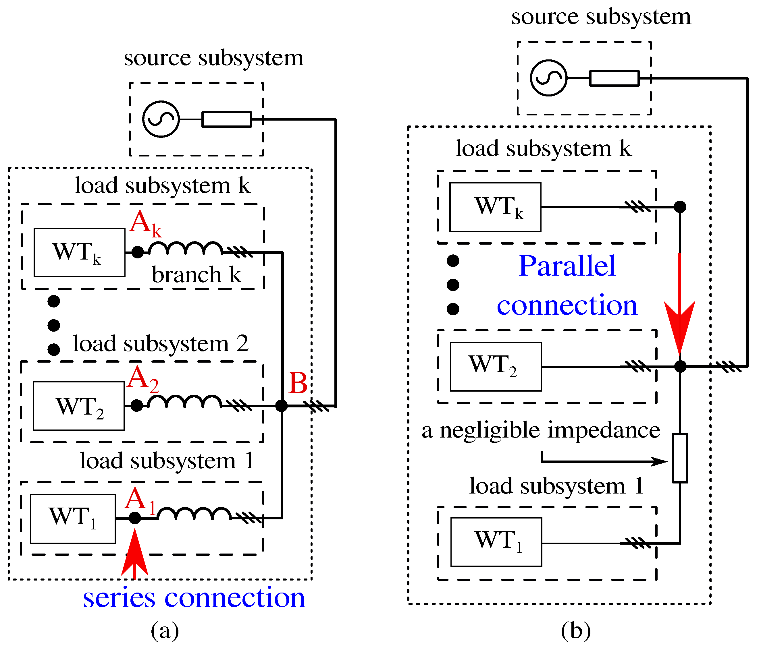
One of the most widely used methods to study this small-signal stability problem is impedance-based analysis. The impedance-based stability analysis method focuses on the terminal characteristic of the subsystems, where the interconnected system can be divided into multiple subsystems and modeled separately [3]. In impedance-based analysis, the subsystems can also be regarded as black boxes, and their terminal frequency domain characteristic can be obtained through a sweep frequency test, which highlights the method’s advantage in practical application. Usually, a power-electronic interfaced wind turbine (WT) is modeled as a load subsystem, which behaves as a current source with an internal parallel connected impedance [4]. The weak grid is modeled as a source subsystem, which behaves as a voltage source with an internal series-connected impedance. If those two internal impedances are not compatible (e.g., when the two internal impedances form a series resonance circuit with negative resistance), then unstable resonance in the interconnected system will occur [3]. Due to its simplicity and good extensibility, impedance-based analysis is also widely applied in system-level analysis where multiple WTs are considered [5,6].

To obtain the impedance model analytically over a wider frequency band, linearization is required. Such a small-signal impedance model can be developed in different domains. Typical domain choices include stationary sequence domain [7] or synchronous DQ domain [8]. Other alternative choices such as modified sequence domain and phasor domain can be found in [9,10]. These models are all two-dimensional in order to capture the terminal frequency response characteristic of the converter. Moreover, linear coordinate transformations are founded to establish their equivalences [10] in single-machine analysis (e.g., grid-connected converter or double-fed induction generator). The developed model does a good job of describing the influence of grid-side converter (GSC) dynamics on the impedance characteristic where phase-locked loop and DC-link voltage control are considered [11,12].

In general, the linearization requires the definition of an operation point. Therefore, the obtained small-signal impedance model is dependent on the expression of an operation point, and is further linked to the choice of reference frame. For studies of single-machine analysis, the reference frame is chosen by assuming that the fundamental voltage at the point of common coupling (PCC) has zero phase angle. However, in multiple-machine analysis, the terminal voltages of each subsystem are not necessary the same due to the line impedance.

The consequences of reference frame mismatch on the impedance model aggregation which is performed in the system-level analysis are discussed in [13,14]. It was shown that the mismatch issue is an obstacle for the simple aggregation of a small-signal impedance model. Though power flow analysis performed in the entire network can solve the mismatch issue, the merits of impedance-based analysis (e.g., simplicity, intuitiveness) are compromised.

One method to avoid the mismatch issue is to adopt the diagonal signal impedance model proposed in [7]. One of the merits of diagonal sequence domain impedance is the irrelevance to reference frame choice which enables its easier expansion to larger systems [2]. Nevertheless, its prediction accuracy becomes poorer when it comes to unstable resonance happening closer to the fundamental frequency, where the unstable resonances have two frequency components symmetrical about the fundamental frequency. This is known as the mirror frequency effect (MFE) [10], which is excluded in the diagonal impedance model. To predict unstable resonance events accurately, the sequence domain impedance model, which is a non-diagonal matrix, is proposed in [15,16].

However, as long as the MFE is considered in the sequence domain model with its two dimensions being coupled, it becomes dependent on the reference frame, just as with the DQ domain one. Hence, the direct connection of these small-signal impedance models without considering the differences among the reference frames of each WT may result in an inaccurate lumped impedance model. This issue is not discussed in [6], where an MFE-included aggregated impedance model of a wind farm is used to study its resonance with the connection to a weak grid.

In order to keep impedance-based analysis simple and intuitive, it is desired to investigate the impedance aggregation method without considering the reference frame issue, as long as the compromise in accuracy is acceptable. Therefore, a comparison between an aggregated type-IV WT impedance model obtained by the accurate aggregation method and the direct aggregation method is presented. The influence of the direct aggregation method on stability analysis is investigated for an interconnected system consisting of a type-IV WT and a weak AC grid.

2. Background on the Impedance Modeling of Multiple WTs

An example of larger-scale wind farms in the sending terminal grid in Xinjiang, China is demonstrated as shown in Figure 1. Four hierarchies can be found considering the impedance aggregation of the wind farms in the sending terminal grid. The lowest level is the single WT, in which WTs are connected to the 35-kV side of a step-up transformer installed in the wind farm terminal. Then, the wind farms are clustered to the substation by a 110-kV transmission line, which is the second level. The third level is composed of the substations, which are connected to the main transformer by a 220-kV transmission line. Finally, the voltage level is increased to 750 kV by the main transformer, and through a long transmission line and another transformer, the sending terminal grid is integrated into the external grid. Thus, the highest level of impedance aggregation is to obtain the terminal characteristic of the whole sending terminal grid.

The impedance aggregation procedure is briefly explained as follows. Firstly, assuming an impedance model of a wind turbine seen from its 690 V terminal is already obtained, to get its impedance model seen from 35 kV at a higher level, it needs to be transformed to the 35 kV side and be series-connected with the impedance model of the transformer and the impedance of the transmission line which connects it to the PCC at 35 kV. Then, the models are lumped with other WT impedance models at 35 kV and an aggregate impedance model of multiple WTs seen from the 35 kV PCC is obtained. Similar steps need to be repeated when aggregating impedance models at 35 kV to higher levels.

During the development of the aggregated impedance model, the involved WTs may have different angle phase of their terminal voltage, indicating that their impedance models are not in a common global frame. Therefore, directly aggregating impedance models from lowest to highest levels will lead to model mismatch. However, if the mismatch is within an acceptable range, then the direct aggregation method is a preferred choice because it usually avoids power flow analysis, which might be complicated and time consuming due to the uncertainty of renewable energy [17,18], and the simplicity of impedance-based analysis will be lost.

Moreover, it is worth mentioning that impedance aggregation is not only about analytical impedance models, but also about impedance models obtained by the impedance sweeping frequency test [19]. In order to be consistent with the analytical model for post validation, the measurement results should meet the assumption that the fundamental voltage at the WT terminal has zero phase angle, which is achieved by adjusting the beginning of fast Fourier transform (FFT) windows. In other words, the WT impedance model obtained by measurement is local-frame-based. It is complicated to obtain impedance models in the global frame by synchronizing the beginning time of all the FFT windows, which in turn shows the significance of investigating the accuracy of the direct impedance aggregation using local impedance models.

3. Reference-Dependent Properties of a Small-Signal Sequence Domain Impedance Model

3.1. Series Connection

The series connection of a small-signal impedance model is illustrated in Figure 2a. Assuming that the terminal voltage of kth WT at point $A_k$ consists of a fundamental frequency component and one pair of small-signal sinusoidal perturbations, it can be expressed in the time domain as:

$$\begin{array}{cc}\hfill v_k^l\left(t\right)& \hfill =V_{1}cos\left({\omega }_{1}t\right)+V_{p}cos\left({\omega }_{p}t+{\varphi }_{vp}\right)\\ \hfill & \hfill +V_{n}cos\left(({\omega }_p-2{\omega }_1)t+{\varphi }_{vn}\right),\end{array}$$

(1)

where $V_1$ is the amplitude of the fundamental voltage; $V_p$ and ${\varphi }_{vp}$ are the amplitude and phase angle of the positive sequence voltage perturbation, respectively; and $V_n$ and ${\varphi }_{vn}$ are the amplitude and phase angle of the negative sequence voltage perturbation, respectively.

The small voltage perturbation in (1) will stimulate a small current response with both positive and negative sequence, which are superposed on the fundamental current and can be expressed as:

$$\begin{array}{cc}\hfill i_k^l\left(t\right)& \hfill =I_{1}cos\left({\omega }_{1}t+{\varphi }_{I1}\right)+I_{p}cos\left({\omega }_{p}t+{\varphi }_{ip}\right)\\ \hfill & \hfill +I_{n}cos\left(({\omega }_p-2{\omega }_1)t+{\varphi }_{in}\right).\end{array}$$

(2)

Then, the impedance model ${\mathit{Z}}_k^l$ of the kth WT maps the small-signal perturbations between current and voltage, and can be represented as:

$$\left[\begin{array}{c}{v}_{p,k}^l\\ v_{n,k}^l\end{array}\right]=\left[\begin{array}{cc}{Z}_{pp,k}& Z_{pn,k}\\ Z_{np,k}& Z_{nn,k}\end{array}\right]\left[\begin{array}{c}{i}_{p,k}^l\\ i_{n,k}^l\end{array}\right],$$

(3)

where

$${[i_{p,k}^l,i_{n,k}^l]}^T={[I_p\angle {\varphi }_{ip},I_n\angle {\varphi }_{in}]}^T,$$

(4)

$${[v_{p,k}^l,v_{n,k}^l]}^T={[V_p\angle {\varphi }_{vp},V_n\angle {\varphi }_{vn}]}^T.$$

(5)

The superscript l shown in (3) indicates that the impedance model of the kth WT is under the assumption that fundamental voltage at $A_k$ has zero phase angle. In other words, the local reference frame of the kth WT is aligned to the fundamental voltage at its own terminal $A_k$, hence (3) is a local-reference-frame-based small-signal model. On the other hand, the impedance model of the connecting component of line $A_{k}B$ shown in Figure 2a can be expressed as:

$$\left[\begin{array}{c}{v}_p-v_{p,k}\\ v_n-v_{n,k}\end{array}\right]=\left[\begin{array}{cc}{Z}_{gpp,k}& 0\\ 0& Z_{gnn,k}\end{array}\right]\left[\begin{array}{c}{i}_{p,k}\\ i_{n,k}\end{array}\right],$$

(6)

where the off-diagonal elements in the impedance matrix are zeros since the connecting components are passive elements (e.g., transmission line or leakage inductance of the transformers), and there is no coupling in their impedance matrices.

To obtain the impedance model of the kth branch seen from point B, the local variables of the kth WT in (3) including the terminal voltage and current need to be transformed to the global reference frame, which can be represented as:

$$\left[\begin{array}{c}{x}_{p,k}^l\\ x_{n,k}^l\end{array}\right]=\left[\begin{array}{cc}{e}^{j{\theta }_k}& 0\\ 0& e^{-j{\theta }_k}\end{array}\right]\left[\begin{array}{c}{x}_{p,k}\\ x_{n,k}\end{array}\right]x=(i,v),$$

(7)

where ${\theta }_k$ is the angular displacement between the phase angle of the fundamental voltage at B which the global frame is aligned to, and the phase angle of the fundamental voltage at $A_k$ which the local frame of the kth WT is aligned to. Note that the impedance-based analysis method requires the separation of the system into one source subsystem and one load subsystem. The global frame is referred to the point where the separation is implemented.

Then, combining (3), (6), and (7), the series-connected impedance model seen from point B can be obtained as:

$$\begin{array}{cc}\hfill \left[\begin{array}{c}{v}_p\\ v_n\end{array}\right]& =\left[\begin{array}{cc}{Z}_{pp,k}+Z_{gpp,k}& Z_{pn,k}{e}^{j2{\theta }_k}\\ Z_{np,k}{e}^{-j2{\theta }_k}& Z_{nn,k}+Z_{gnn,k}\end{array}\right]\left[\begin{array}{c}{i}_{p,k}\\ i_{n,k}\end{array}\right]={\mathit{Z}}_s\left[\begin{array}{c}{i}_{p,k}\\ i_{n,k}\end{array}\right].\hfill \end{array}$$

(8)

In contrast, the direct series connection of impedance models (3) and (6) can be expressed as:

$$\begin{array}{cc}\hfill \left[\begin{array}{c}{v}_p\\ v_n\end{array}\right]=& \left[\begin{array}{cc}{Z}_{pp,k}+Z_{gpp,k}& Z_{pn,k}\\ Z_{np,k}& Z_{nn,k}+Z_{gnn,k}\end{array}\right]\left[\begin{array}{c}{i}_{p,k}\\ i_{n,k}\end{array}\right]={\mathit{Z}}_s^l\left[\begin{array}{c}{i}_{p,k}\\ i_{n,k}\end{array}\right].\hfill \end{array}$$

(9)

It can be found that in (9) the angle of $Z_{np,k}$ is $2{\theta }_k$ lagging while the angle of $Z_{pn.k}$ is $2{\theta }_k$ leading, resulting in inaccurate modeling of the MFE.

The above analysis of error caused by local model aggregation was verified by a sweeping frequency simulation of a 1.5-MW Type IV wind turbine connected to the grid through a transformer. The short-circuit impedance of the 690 V/35 kV transformer was 6.67%. It can be found in Figure 3 that the local impedance model aggregation consisting of a Type IV wind turbine and transformer could achieve an accurate admittance of diagonal element $Y_{pp}$. However, for the off-diagonal element $Y_{pn}$, though its amplitude was well fitted, there were constant errors between the analytical phase model and the simulation result, which validates the accuracy analysis of the series-connected impedance model shown in (8) and (9).

3.2. Parallel Connection

The parallel connection of a small-signal impedance model is illustrated in Figure 2b. The kth WT can be expressed as:

$$\left[\begin{array}{c}{i}_{p,k}\\ i_{n,k}\end{array}\right]=\left[\begin{array}{cc}{Y}_{pp,k}& Y_{pn,k}\\ Y_{np,k}& Y_{nn,k}\end{array}\right]\left[\begin{array}{c}{v}_p\\ v_n\end{array}\right].$$

(10)

Unlike series connection, the two components connected in parallel are subjected to the same voltage perturbation ${\left[\begin{array}{cc}{v}_p& v_n\end{array}\right]}^T$. Besides, the current response $i_p$ and $i_n$ of WTs in parallel can be calculated as:

$${\left[\begin{array}{cc}{i}_p& i_n\end{array}\right]}^T=\sum {\left[\begin{array}{cc}{i}_{p,k}& i_{n,k}\end{array}\right]}^T.$$

(11)

Then, the admittance matrix of the aggregated system is the sum of the two WTs, which can be represented as:

$${\left[\begin{array}{cc}{Y}_{pp}& Y_{pn}\\ Y_{np}& Y_{nn}\end{array}\right]}^T=\sum {\left[\begin{array}{cc}{Y}_{pp,k}& Y_{pn,k}\\ Y_{np,k}& Y_{nn,k}\end{array}\right]}^T.$$

(12)

If the line impedance between nearby WTs in the wind farm is negligible, as illustrated in Figure 2b, the admittance model of the wind farm containing identical WTs can be expressed as:

$${\left[\begin{array}{cc}{Y}_{pp}& Y_{pn}\\ Y_{np}& Y_{nn}\end{array}\right]}^T={\left[\begin{array}{cc}n{Y}_{pp,k}& n{Y}_{pn,k}\\ n{Y}_{np,k}& n{Y}_{nn,k}\end{array}\right]}^T,$$

(13)

where n is the number of WTs inside the wind farm.

3.3. Combination of Series Connection and Parallel Connection

For typical impedance model aggregation applications such as the one shown in Figure 1, the impedance aggregation model can be expressed as:

$${\mathit{Z}}_{agg}=\stackrel{k}{\underset{n=1}{\mathrm{Parallel}}}\left(\mathrm{series}\left({\mathit{Z}}_k,{\mathit{Z}}_{ck},{\theta }_k\right)\right),$$

(14)

where the function “series” describes the series connection of the impedance ${\mathit{Z}}_k$ of the kth WT, ${\mathit{Z}}_{ck}$ is the impedance model including transmission lines and the transformer which connects ${\mathit{Z}}_k$ to a higher hierarchy. ${\theta }_k$ is the reference frame mismatch between the global one and the local one, which is set to zero in the direct series connection method. The function “parallel” describes the parallel connection of impedance models of n subsystems. ${\mathit{Z}}_{agg}$ is the aggregated impedance model of n parallel branches. An example scenario is that the impedance models of WTs are series-connected to the leakage inductance of the step-up transformer before they are connected in the AC bus.

In Section 2, it was pointed out that for off-diagonal elements, the direct series connection of two impedance models will lead to the phase error, while the amplitude correctness is kept. However, when further connection such as (14) is applied, the mismatch can also be found in the impedance amplitude.

The accurate method of impedance aggregation can be written as:

$$\begin{array}{cc}\hfill Y_{pn}& ={\displaystyle \sum _{k=1}^n}{Y}_{pn,k}={\displaystyle \sum _{k=1}^n}{Y}_{pn,k}^l{e}^{j2{\theta }_k},\hfill \\ \hfill Y_{pn}& ={\displaystyle \sum _{k=1}^n}{Y}_{pn,k}={\displaystyle \sum _{k=1}^n}{Y}_{pn,k}^l{e}^{-j2{\theta }_k}.\hfill \end{array}$$

(15)

The result of the direct impedance aggregation which neglects differences between the local reference frame and the global reference frame can be written as:

$$Y_{pn}^l=\sum _{k=1}^n{Y}_{pn,k}^l{Y}_{np}^l=\sum _{k=1}^n{Y}_{np,k}^l.$$

(16)

According to (15) and (16), $Y_{pn}^l$ and $Y_{pn}$ are usually different unless the angular displacement ${\theta }_k$ between the global frame and the local frame is the same for all branches.

3.4. Discussion of the Mismatch Caused by Model Connection

During the impedance aggregation of WTs, plenty of serial connections will exist due to the line impedance and leakage inductance of the transformers, which will affect the aggregation accuracy of the impedance model.

On one hand, in some cases, the accuracy influence due to the reference frame issue may be ignored. According to (8), the mismatch will be acceptable if either the amplitude of off-diagonal elements is negligible or the angle differences ${\theta }_k$ among branches are very small.

The example for the first case is that WT has conservative PLL design and strong DC-link, in which off-diagonal elements in the impedance model can be neglected due to much smaller amplitude [7]. As a result, the conventional sequence domain impedance proposed in [7], without off-diagonal terms, can be treated as a passive impedance element because this kind of model can be connected in series without losing accuracy.

The example for the second case is that of the impedance model aggregation inside one wind farm. Due to the small length of connection line between nearby WTs, the WTs share almost the same voltage perturbation at their terminals. Then, the direct aggregation methods of the small-signal impedance model can be applied to WTs inside the wind farm.

On the other hand, there are also cases where the grid-connected WTs have a coupling characteristic where the amplitude of off-diagonal elements is considerable, especially around fundamental frequency [15,16], or the voltage drop across the connection line becomes larger in a weaker grid network. In all these scenarios, it is necessary to investigate how the accuracy of the direct aggregated impedance model will be affected and how these mismatches affect the impedance-based stability analysis. Therefore, in order to keep the advantage of impedance-based stability analysis, the side effect of the direct impedance aggregation methods on stability analysis needs to be evaluated in the practical application.

4. Impedance Model Aggregation of a Type-IV WT

Because the reference frame mismatch issue is related to the off-diagonal elements of the impedance model, in order to analyze its impact on the stability of interconnection between type-IV WTs and the weak grid, the characteristic of the off-diagonal element of the type-IV WT impedance model needs to be investigated first.

The type-IV WT analyzed in this paper is interfaced with the grid by a GSC. The topology and the control system of the GSC are depicted in Figure 4. The $v_{rdc}$ is the reference of DC-link voltage. The desired terminal voltage of the converter is represented by $m_{abc}$, and it is realized as the terminal voltage of the converter $e_{abc}$, which is generated by pulse width modulation (PWM). The PWM process and digital control delay can be expressed as $e_x=e^{-1.5T_{sw}s}{K}_m{m}_x(x=a,b,c)$ in average model development, where $T_{sw}$ is the switching frequency and $K_m$ is the modulation index.

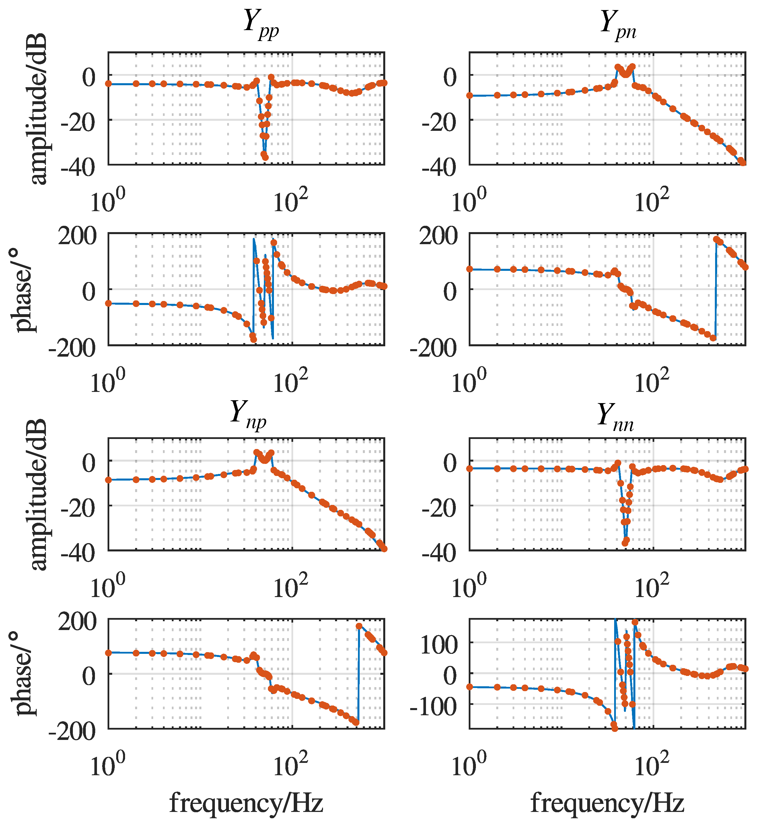
According to the impedance modelling method proposed in [20], the analytical impedance model of a GSC can be developed by a $2\times 2$ matrix, which is verified by a sweeping test in the simulation, as demonstrated in Figure 5. The parameters of the GSC are listed in

Table 1. GSC parameters.

Parameter	Symbol	Value
Filter inductance	$L_f$	0.25 mH
Filter capacitor	$C_f$	500 mF
Damping resistor	$R_f$	0.5 $\Omega$
DC-link capacitor	$C_{dc}$	50 mF
Output resistor	$R_d$	0.001
Current controller proportional gain	$k_{pi}$	1.56
Current controller integral gain	$k_{ii}$	182.62
DC voltage controller proportional gain	$k_{pv}$	1
DC voltage controller integral gain	$k_{iv}$	100
Phase-locked loop (PLL) filter proportional gain	$k_{pp}$	138
PLL loop filter integral gain	$k_{ip}$	1380
Switching frequency	$T_{sw}$	5 kHz

.

It can be observed that the off-diagonal elements in admittance matrix had comparable or even larger amplitude than the diagonal elements near fundamental frequency, which indicates that within the frequency band near fundamental frequency, the frequency domain characteristics of a WT terminal can be largely affected by off-diagonal admittance elements. In the frequency band away from the fundamental frequency, the amplitude of off-diagonal elements quickly rolled off, and the small-signal admittance model of the WT had negligible MFE, and behaved like a passive impedance element. According to (8), the reference frame mismatch issue should be considered only when off-diagonal elements dominate over the characteristic of the impedance matrix. In other words, when it comes to the investigation of reference frame mismatch, the frequency band of interest is the one around the fundamental frequency, where off-diagonal elements have much higher amplitude than diagonal elements.

The stability of the interconnected system consisting of a weak grid and a single GSC is determined by their impedance ratio [4]. If the eigenloci of the impedance ratio encircles (−1,0) in the complex plane, the interconnected system is unstable. Both the load subsystem WT and source subsystem have $2\times 2$ impedance matrix, and their impedance ratio $\mathit{L}$ can be calculated as:

$$\mathit{L}=\left[\begin{array}{cc}{L}_{pp}& L_{pn}\\ L_{np}& L_{nn}\end{array}\right]=\mathit{Y}{\mathit{Z}}_{\mathit{g}}=\left[\begin{array}{cc}{Y}_{pp}{Z}_{gp}& Y_{pn}{Z}_{gn}\\ Y_{np}{Z}_{gp}& Y_{nn}{Z}_{gn}\end{array}\right],$$

(17)

where the impedance of the source subsystem ${\mathit{Z}}_{\mathit{g}}$ was assumed to be passive impedance with zero off-diagonal elements in this paper.

The impedance ratio shown in (17) has two eigenloci ${\lambda }_1$ and ${\lambda }_2$, which can be expressed as:

$$\begin{array}{cc}\hfill {\lambda }_{1,2}=& {\displaystyle \frac{L_{pp}+L_{nn}\pm \sqrt{{(L_{pp}-L_{nn})}^2+4L_{pn}{L}_{np}}}{2}}.\hfill \end{array}$$

(18)

When the GSC with impedance characteristic shown in Figure 5 is connected to a weak grid where the SCR is 1.56, the eigenloci of the interconnected system are shown in Figure 6. It is observed that the eigenloci near fundamental frequency were closest to (−1,0) where the system stability margin was very limited.

The influence of off-diagonal elements on the stability analysis can be illustrated by the comparison of eigenloci near the fundamental frequency shown in Figure 7, in which the simplified eigenloci neglecting off-diagonal GSC admittance elements are represented as:

$$\begin{array}{cc}\hfill {\lambda }_{diag,1,2}=& {\displaystyle \frac{L_{pp}+L_{nn}\pm \sqrt{{(L_{pp}-L_{nn})}^2}}{2}}.\hfill \end{array}$$

(19)

It can be observed that the simplified eigenloci were far away from (−1,0). Therefore, it can be concluded that the off-diagonal elements were responsible for pushing the eigenloci near the fundamental frequency to (−1,0). In other words, the eigenloci were largely affected by the term $4L_{pn}{L}_{np}$ which is associated with the off-diagonal elements $Y_{pn}$ and $Y_{np}$ of the GSC. Therefore, the off-diagonal elements of the GSC admittance model play an important role in stability analysis, especially in predicting the stability problem around the fundamental frequency.

Furthermore, since the amplitude of eigenloci, approximated by $|L_{pn}{L}_{np}|$, is proportional to |$Y_{pn}{Y}_{np}$|, there is a positive correlation between the amplitude of eigenloci and the amplitude of off-diagonal elements in the WT impedance model. The smaller amplitude of eigenloci near the fundamental frequency will make them move away from (−1,0). Thus, it can be concluded that a smaller amplitude of off-diagonal admittance elements leads to a larger stability margin of the interconnected system around the fundamental frequency, which is illustrated in Figure 7, showing that eigenloci shrank as the amplitude of off-diagonal WT admittance reduced.

It should also be pointed out that the phase mismatch shown in the off-diagonal elements can be canceled when calculating eigenloci (18), which can be expressed as:

$$\begin{array}{c}\hfill Y_{pn}^l{e}^{j2{\theta }_k}{Y}_{np}^l{e}^{-j2{\theta }_k}=Y_{pn,k}^l{Y}_{np,k}^l\end{array}.$$

(20)

Therefore, the phase mismatch does not degrade the precision of the stability analysis. Practically, there are huge numbers of WTs integrated in the wind farm. To simplify the stability analysis, the assumption was made here that all WTs had the same control parameters and power factor control mode. The only difference between them was the active power reference which could be different due to wind energy distribution.

Figure 8 shows how the active power influenced the off-diagonal elements of the WT admittance model. It is demonstrated that greater active power output increased the amplitude of off-diagonal elements, while it had little impact on the phase of the off-diagonal elements, especially inside the frequency band of interest, around the fundamental frequency. This is illustrated by the interval defined by two dotted lines shown in Figure 8, where off-diagonal elements had higher amplitude. If the impedance of each wind farm was approximated by the impedance model of an equivalent WT with the same power rating, it can be inferred that impedance models of wind farms would have similar phase characteristic of their off-diagonal elements. The amplitude of off-diagonal elements in the impedance models of wind farms are positively correlated to their active power.

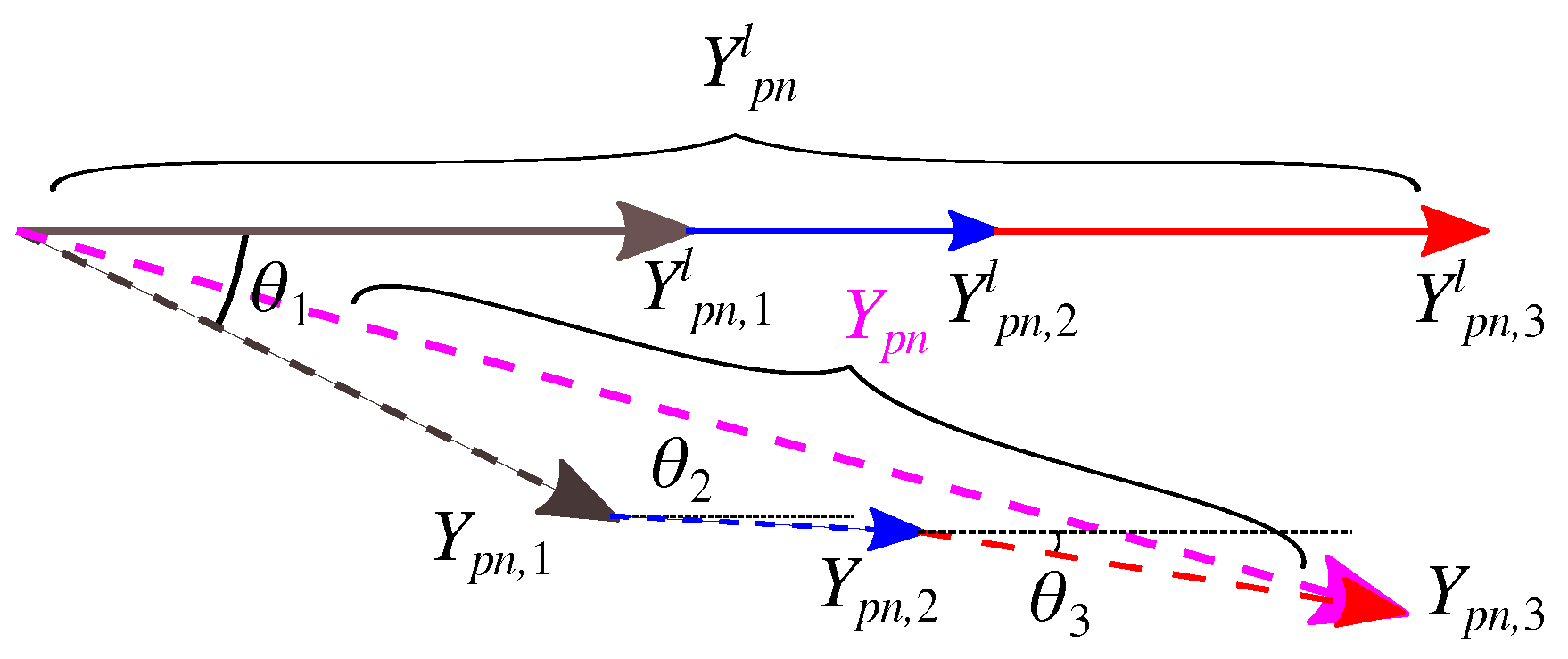
Therefore, if the impedance models of the wind farms are aggregated, the aggregation can be illustrated by the vector diagram shown in Figure 9 in the case of three-branch aggregation. The key point is that every $Y_{pn,k}^l$ is in the same direction due to their same phase angle in the frequency band of interest. Besides, their active power outputs are presented by the length of their vectors. As illustrated in Figure 9, the amplitude error between the accurate model and the one obtained by local model aggregation can be calculated as:

$$|Y_{pn}|-|Y_{pn}^l|=|Y_{pn}|-|\sum _{k=1}^n|Y_{pn,k}^l|e^{j{\theta }_k}|.$$

(21)

It can be observed in (21) that the amplitude of the off-diagonal elements of an accurate impedance model will be shorter than the one obtained by the direct aggregation method. The mismatch could be subtle if ${\theta }_k$ are similar to each other, even if all of them are not small. An indicator J can be defined by calculating the mean amplitude error of off-diagonal elements over frequency band $[f_1,f_2]$ where reference frame issue matters, and expressed as:

$$\begin{array}{c}\hfill J=\frac{1}{N}{\displaystyle \sum _{k=1}^N}\left(\left(|Y_{pn}\left(f_k\right)|-|Y_{pn}^l\left(f_k\right)|\right)/\left|Y_{pn}\left(f_k\right)\right|\right)\\ \hfill f_k=\frac{N-k}{N}{f}_1+\frac{k}{N}{f}_2.\end{array}$$

(22)

The amplitude of the off-diagonal elements is a critical factor in the prediction of the stability margin near fundamental frequency. Larger J indicates poorer accuracy of the stability analysis obtained by the direct impedance aggregation.

5. Impedance Modeling of Multiple WTs in a Wind Farm

The case shown in Figure 1 is studied here at the substation level. The impedance model of all substations seen from main transformer at 220 kV side was built. The base power was set as 4000 MW and the base voltage was set as 220 kV. The parameters of the case are listed in

Table 2. Parameters of the case shown in Figure 1.

Substation	1	2	3	4
Line resistance (p.u.)	0.018	0.028	0.042	0.042
Line Inductance (p.u.)	0.830	1.258	1.405	1.523
Active power (p.u.)	0.325	0.225	0.313	0.138
Reference frame mismatch (°)	15.51	16.367	28.104	11.793

.

The angle displacements between the four local reference frames of each subsystem and the global reference frame were calculated using power flow calculation and are listed in Table 2. The error indicator $J_1$ was calculated over the frequency band [40 Hz, 60 Hz] and it was equal to 0.0633. The comparison between the local-reference-based lumped wind farm impedance model and the global-reference-based lumped wind farm impedance model about off-diagonal elements and eigenloci is shown in Figure 10, where grid impedance had 0.058 p.u. resistance and 0.423 p.u. reactance. It was found that although there was a phase mismatch of about ${30}^{°}$ in off-diagonal element modeling, the eigenloci of two models were almost identical. It is demonstrated that when branches in the system were loaded in balance, the mismatch of the reference frame hardly perturbed the eigenloci of the system. In other words, the stability analysis results obtained by aggregating local models and aggregating the global-reference-frame-based models were the same. In this circumstances, the direct impedance model is preferred because it avoids power flow analysis.

However, if the active power distribution among the four substations changes, the accuracy of the stability analysis with the direct impedance aggregation method will also be changed, which could be reflected by a changed error indicator J. Here the active power generation of substation 2 was kept as 900 MW and the remaining 3100 MW was redistributedamong the other three substations. The relationship between active power distribution and the error indicator J is presented in Figure 11. It was observed that a small indicator J could be found in most situations of active power distribution, since most of the surface of J shown in Figure 11 is rendered by deep blue. Therefore, the inaccuracy in the stability analysis due to impedance model mismatch caused by the direct aggregation method should be ignored, which is similar to that demonstrated in the previous case.

Nevertheless, J could increase to above 0.2 when substation 3 with a relatively large transmission line impedance was heavy loaded. The increase of J was alleviated when substation 1 was heavily loaded, since the voltage angle difference between the connection line became smaller because the impedance of the transmission line connecting substation 1 was the smallest one in the studied case.

To show the consequence of an increased indicator J, the stability analysis was carried out on another active power distribution with $J=0.2072$, whose parameters are shown in

Table 3. Parameters of configuration where error indicator $J_2=0.2072$.

Substation	1	2	3	4
Active power (p.u.)	0.325	0.225	0.313	0.16
Reference frame mismatch (°)	4.690	16.098	44.606	13.813

. Comparing it to the first case shown in Table 2, the active power in substation 3 increased to about half of the total active power generated by the whole wind farm cluster. In Figure 12, two eigenloci—one obtained by the accurate aggregated impedance model and the other obtained by the direct aggregated impedance—are presented, where the grid impedance had 0.134 p.u. resistance and 0.972 p.u. reactance. Instability was predicted according to the eigenloci of the direct aggregated model, which encircles (−1,0). However, due to eigenloci expansion explained previously, there was still some stability margin left predicted by the accurate aggregated impedance model, though it was not large.

The above stability analysis was validated by the time-domain simulation shown in Figure 13, where the system kept stable when the active power of the whole wind farm stepped from 1.0 p.u. to 1.06 p.u. at 1 s, though an apparent overshoot of the output current indicates that the system margin was not large.

6. Conclusions

The model of WTs’ sequence domain small-signal impedance characteristic is dependent on the local reference frame. Directly connecting the WT impedance model with other impedance models in the sending terminal grid will lead to inaccuracy in the modeling of off-diagonal admittance elements due to the reference frame mismatch, which is caused by the voltage angle differences among the aggregated subsystems. The accuracy of stability analysis was investigated, considering the mismatch between the accurate impedance model built by the impedance aggregation method considering reference frame mismatch and the simplified impedance model built by the direct aggregation method. It was found that the extent of mismatch was related to active power flow. The impact of reference frame mismatch on the impedance-based stability tended to be subtle in common configuration where branches are loaded in balance. Therefore, direct impedance model aggregation can be applied with confidence in its accuracy for common applications. Nevertheless, attention still needs to be paid to inaccurate stability analysis when some branches are extremely heavily loaded.

References

1. Zhao, M.; Yuan, X.; Hu, J.; Yan, Y. Voltage Dynamics of Current Control Time-Scale in a VSC-Connected Weak Grid. IEEE Trans. Power Syst. 2016, 31, 2925–2937. [Google Scholar] [CrossRef]
2. Sun, J.; Li, M.; Zhang, Z.; Xu, T.; He, J.; Wang, H.; Li, G. Renewable energy transmission by HVDC across the continent: System challenges and opportunities. CSEE J. Power Energy Syst. 2017, 3, 353–364. [Google Scholar] [CrossRef]
3. Sun, J. Impedance-Based Stability Criterion for Grid-Connected Inverters. IEEE Trans. Power Electron. 2011, 26, 3075–3078. [Google Scholar] [CrossRef]
4. Sun, J. Small-Signal Methods for AC Distributed Power Systems—A Review. IEEE Trans. Power Electron. 2009, 24, 2545–2554. [Google Scholar]
5. Kunjumuhammed, L.P.; Pal, B.C.; Gupta, R.; Dyke, K.J. Stability Analysis of a PMSG-Based Large Offshore Wind Farm Connected to a VSC-HVDC. IEEE Trans. Energy Convers. 2017, 32, 1166–1176. [Google Scholar] [CrossRef]
6. Wang, H.; Vieto, I.; Sun, J. A Method to Aggregate Turbine and Network Impedances for Wind Farm System Resonance Analysis. In Proceedings of the 2018 IEEE 19th Workshop on Control and Modeling for Power Electronics (COMPEL), Padova, Italy, 25–28 June 2018. [Google Scholar]
7. Cespedes, M.; Sun, J. Impedance Modeling and Analysis of Grid-Connected Voltage-Source Converters. IEEE Trans. Power Electron. 2014, 29, 1254–1261. [Google Scholar] [CrossRef]
8. Wen, B.; Boroyevich, D.; Burgos, R.; Mattavelli, P.; Shen, Z. Analysis of D-Q Small-Signal Impedance of Grid-Tied Inverters. IEEE Trans. Power Electron. 2016, 31, 675–687. [Google Scholar] [CrossRef]
9. Shah, S.; Parsa, L. Impedance Modeling of Three-Phase Voltage Source Converters in DQ, Sequence, and Phasor Domains. IEEE Trans. Energy Convers. 2017, 32, 1139–1150. [Google Scholar] [CrossRef]
10. Rygg, A.; Molinas, M.; Zhang, C.; Cai, X. A Modified Sequence-Domain Impedance Definition and Its Equivalence to the dq-Domain Impedance Definition for the Stability Analysis of AC Power Electronic Systems. IEEE J. Emer. Sel. Top. Power Electron. 2016, 4, 1383–1396. [Google Scholar] [CrossRef]
11. Zhang, C.; Cai, X.; Molinas, M.; Rygg, A. On the Impedance Modeling and Equivalence of AC/DC-Side Stability Analysis of a Grid-Tied Type-IV Wind Turbine System. IEEE Trans. Energy Convers. 2019, 34, 1000–1009. [Google Scholar] [CrossRef]
12. Liu, H.; Xie, X.; Liu, Z. Comparative Studies on the Impedance Models of VSC-Based Renewable Generators for SSI Stability Analysis. IEEE Trans. Energy Convers. 2019. [Google Scholar] [CrossRef]
13. Rygg, A.; Molinas, M.; Unamuno, E.; Zhang, C.; Cai, X. A simple method for shifting local dq impedance models to a global reference frame for stability analysis. arXiv 2017, arXiv:abs/1706.08313. [Google Scholar]
14. Zhang, C.; Molinas, M.; Rygg, A.; Cai, X. Impedance-based Analysis of Interconnected Power Electronics Systems: Impedance Network Modeling and Comparative Studies of Stability Criteria. IEEE J. Emerg. Sel. Top. Power Electron. 2019. [Google Scholar] [CrossRef]
15. Bakhshizadeh, M.K.; Wang, X.; Blaabjerg, F.; Hjerrild, J.; Kocewiak, L.; Bak, C.L.; Hesselbæk, B. Couplings in Phase Domain Impedance Modeling of Grid-Connected Converters. IEEE Trans. Power Electron. 2016, 31, 6792–6796. [Google Scholar]
16. Xu, Y.; Nian, H.; Wang, T.; Chen, L.; Zheng, T. Frequency Coupling Characteristic Modeling and Stability Analysis of Doubly Fed Induction Generator. IEEE Trans. Energy Convers. 2018, 33, 1475–1486. [Google Scholar] [CrossRef]
17. Segura-Heras, I.; Escrivá-Escrivá, G.; Alcázar-Ortega, M. Wind farm electrical power production model for load flow analysis. Renew. Energy 2011, 36, 1008–1013. [Google Scholar] [CrossRef] [Green Version]
18. Li, Q.; Zhang, Y.; Ji, T.; Lin, X.; Cai, Z. Volt/Var Control for Power Grids With Connections of Large-Scale Wind Farms: A Review. IEEE Access 2018, 6, 26675–26692. [Google Scholar] [CrossRef]
19. Luhtala, R.; Roinila, T.; Messo, T. Implementation of Real-Time Impedance-Based Stability Assessment of Grid-Connected Systems Using MIMO-Identification Techniques. IEEE Trans. Ind Appl. 2018, 54, 5054–5063. [Google Scholar] [CrossRef]
20. Shah, S.; Parsa, L. Sequence domain transfer matrix model of three-phase voltage source converters. In Proceedings of the 2016 IEEE Power and Energy Society General Meeting (PESGM), Atlanta, GA, USA, 17–21 July 2016. [Google Scholar]
Figure 1. System topology of a wind farm. The long transmission line and lines inside wind turbine (WT) strings are not drawn proportionally.
Energies 12 02035 g001
Figure 2. (a) Series connection of the impedance model; (b) Parallel connection of the impedance model.
Energies 12 02035 g002
Figure 3. Impedance comparison between analytical model and simulation results. Line with dots: series impedance model obtained by connecting impedance models in local frames; Line with plus signs: series impedance model obtained in global frame.
Energies 12 02035 g003
Figure 4. Control diagram of a grid-side converter (GSC) in a type-IV WT.
Energies 12 02035 g004
Figure 5. Bode diagram of a WT admittance model. Lines: analytic results; Dots: simulation results.
Energies 12 02035 g005
Figure 6. The eigenloci of the interconnected system of a GSC and a weak grid where SCR = 1.56.
Energies 12 02035 g006
Figure 7. The impact of off-diagonal elements on the eigenloci near the fundamental frequency. The displayed frequency band is [30 Hz, 70 Hz].
Energies 12 02035 g007
Figure 8. Bode diagram of off-diagonal GSC admittance elements against active power variation. The dashed line is the amplitude of diagonal elements indicating the weight of off-diagonal admittance elements on the overall terminal frequency characteristic of the GSC.
Energies 12 02035 g008
Figure 9. Off-diagonal element aggregation of substations.
Energies 12 02035 g009
Figure 10. Eigenloci of interconnected system where the error indicator J 1 = 0.10633. (a) Bode diagram of off-diagonal element Y p n . Line: local-reference-frame-based impedance model; Dashed-dotted line: global-reference-frame-based impedance model. (b) Eigenloci of interconnected system. Line with triangles: eigenloci calculated according to local reference frame; Line with circles: eigenloci calculated according to global reference frame.
Energies 12 02035 g010
Figure 11. Error indicator J versus active power distribution among substations 1, 3, and 4.
Energies 12 02035 g011
Figure 12. Eigenloci of an interconnected system where the error indicator J 2 = 0.2072 . Line with triangles: eigenloci calculated according to the accurate aggregated model. Line without triangles: eigenloci calculated according to the direct aggregated model.
Energies 12 02035 g012
Figure 13. Simulation results of wind farm clusters connected to the weak grid where the error indicator J 2 = 0.2072 .
Energies 12 02035 g013