Stochastic Adaptive Robust Dispatch for Virtual Power Plants Using the Binding Scenario Identification Approach

Abstract

The present study establishes a stochastic adaptive robust dispatch model for virtual power plants (VPPs) to address the risks associated with uncertainties in electricity market prices and photovoltaic (PV) power outputs. The model consists of distributed components, such as the central air-conditioning system (CACS) and PV power plant, aggregated by the VPP. The uncertainty in the electricity market price is addressed using a stochastic programming approach, and the uncertainty in PV output is addressed using an adaptive robust approach. The model is decomposed into a master problem and a sub-problem using the binding scenario identification approach. The binding scenario subset is identified in the sub-problem, which greatly reduces the number of iterations required for solving the model, and thereby increases the computational efficiency. Finally, the validity of the VPP model and the solution algorithm is verified using a simulated case study. The simulation results demonstrate that the operating profit of a VPP with a CACS and other aggregated units can be increased effectively by participating in multiple market transactions. In addition, the results demonstrate that the binding scenario identification algorithm is accurate, and its computation time increases slowly with increasing scenario set size, so the approach is adaptable to large-scale scenarios.

1. Introduction

With the growth of electricity demand, fossil fuels have been widely used for electricity generation in recent years as the cheapest source of energy. However, the use of fossil fuels causes a variety of environmental effects and may endanger human health [1,2]. In order to meet the challenges associated with energy shortages and environmental pollution, the world-wide energy production infrastructure is slowly moving in the direction of clean and low-carbon options based on renewable energy sources (RESs) [3,4]. However, RESs suffer from the disadvantages of strong randomness, high volatility, and weak controllability. Therefore, the continuous expansion of grid-connected electric power facilities based on RESs poses a challenge to the safe and reliable operation of electric power grids [5,6,7]. Virtual power plants (VPPs) have been developed to address this challenge. Through advanced control, measurement, and communication technologies, a large number of RESs, controllable loads, energy storage systems (ESSs), and other distributed energy resources are aggregated by VPPs to participate in the power grid operation as a whole, which is conducive to the rational allocation and utilization of resources [8,9,10,11].

In general, a VPP framework promotes the aggregation of various resources by simultaneously participating in multiple markets, such as the day-ahead energy market (DAM) and real-time energy market (RTM), which can improve the flexibility of scheduling [12]. Existing studies have mostly only considered VPP participation in the DAM, and participation has been rarely extended to multiple markets. For example, a VPP model that considers only DAM participation has been established, where the overall demand response (DR) was divided into incentive-based DR and price-based DR mechanisms [13,14,15]. A DR was also applied in a multi-market model, where a VPP participates in both the DAM and RTM simultaneously [12,16]. However, the DR in the above studies was regarded strictly as an interruptible/transferable load, and no specific modeling analysis was applied.

Meanwhile, VPP operations are impacted by uncertain factors such as RES outputs in the scheduling process, resulting in economic and security issues. Therefore, addressing uncertain factors in VPP operations has become a topic of increasing interest [17,18]. Numerous approaches have been applied toward addressing uncertainty in VPP operations, such as stochastic programming [19,20,21], robust optimization [22], chance-constrained programming [23], and point estimation [24]. In contrast, the application of adaptive robust optimization has been relatively rare in this case. However, this approach is more flexible than robust optimization because the decision making process is conducted in stages, which to some extent can alleviate the conservativeness of robust optimization solutions.

Adaptive robust optimization considers the optimal solution under the worst-case conditions of uncertain factors and is generally divided into two stages for decision making [25,26]. The first stage employs what are denoted as here-and-now variables to make decisions before the level of uncertainty is known. The second stage employs what are denoted as wait-and-see variables to make decisions after the level of uncertainty is known. For example, an adaptive robust unit commitment model was established to account for uncertainties in wind power output by the active regulation of pumped storage power stations [27], and an adaptive robust reactive power optimization model was proposed to address the uncertainties in wind power output under conditions of high wind power penetration integrated into active distribution networks [28].

At present, numerous methods have been applied for solving adaptive robust models, such as the affine policy, Benders decomposition, the column and constraint generation (CCG) algorithm, and scenario-based algorithm. The affine policy method uses the linear decision rule to establish the affine relationship between decision variables and uncertain parameters and transforms the two-stage problem into a single-stage problem [29]. However, the results are conservative. A Benders/CCG algorithm has been adopted for decomposing an original stochastic adaptive robust model problem into a master problem and a sub-problem, but the Karush–Kuhn–Tucker (KKT) or duality method was needed to transform the sub-problem into a single-level model, and a large number of integer terms were introduced in the linearization process, leading to high model solution complexity in large-scale problems [30,31]. The scenario-based algorithm was employed to transform a three-level adaptive robust model into a single-level model by enumerating the uncertainty set based on the scenarios [32]. However, the computational efficiency of the scenario-based algorithm decreases as the scale of the problem increases compared with the binding scenario identification approach. This is particularly the case for large-scale scenario sets, where the number of scenarios required for solving the problem is quite large, resulting in a very large computational burden [33,34].

Based on the above analysis, the present study considers a VPP that aggregates a photovoltaic (PV) power plant, a gas turbine, an ESS, a central air-conditioning system (CACS), and interruptible load, and simultaneously participates in multiple market transactions in the DAM, RTM, and carbon trading market (CTM). The contributions of this paper can be briefly summarized as follows:

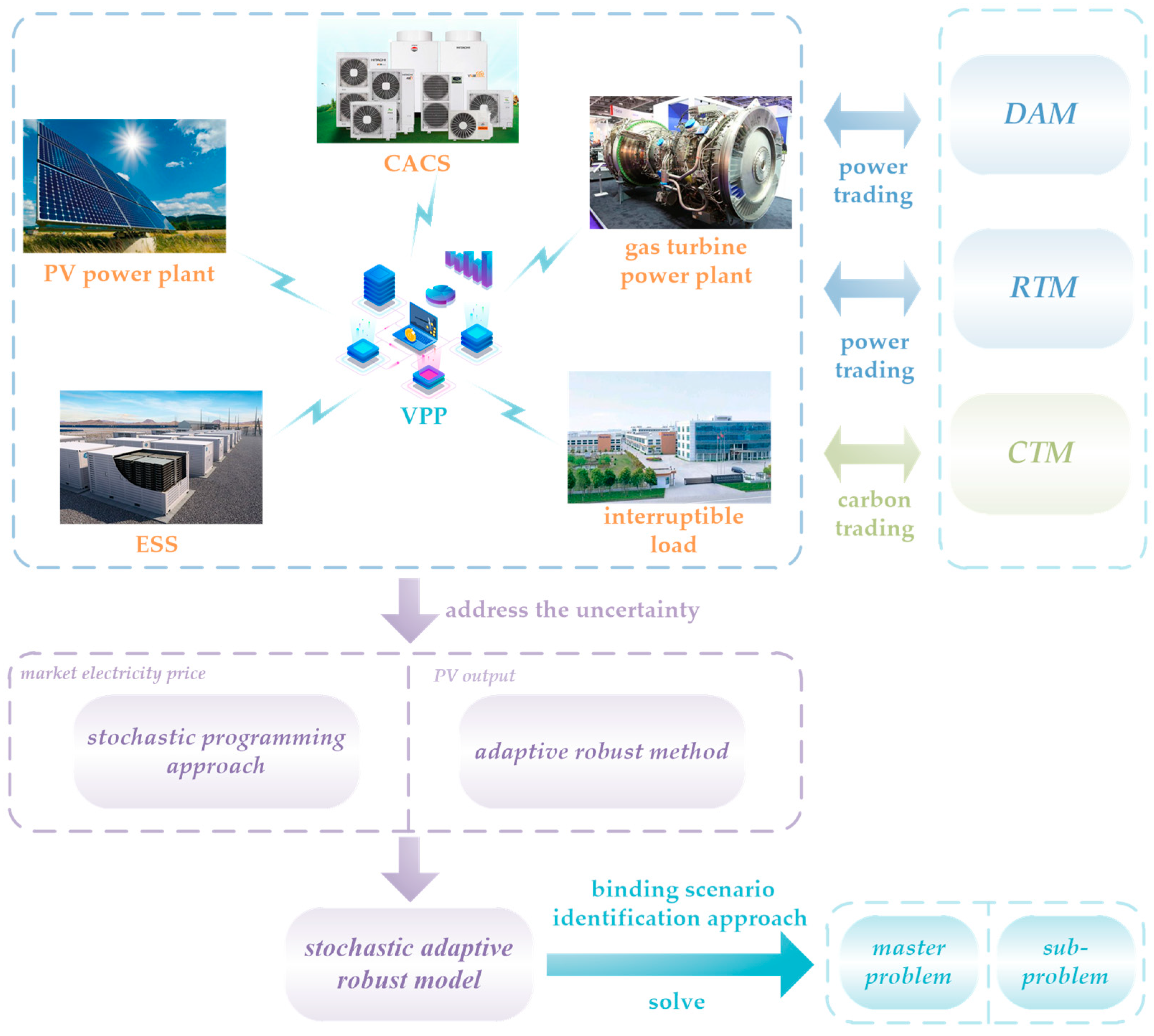
• This paper establishes a stochastic adaptive robust model for VPP dispatch that considers CACS and multiple markets. The stochastic programming approach is used to address the uncertainty of market electricity price owing to the high accuracy of market price forecasting, and the adaptive robust method is used to address the uncertainty of PV output owing to the low accuracy of PV output forecasting.
• The binding scenario identification approach is used to solve the stochastic adaptive robust model for VPP dispatch. The original problem is decomposed into a master problem for solving the single-level optimization model with the binding scenario subset and a sub-problem for identifying the binding scenario subset, which greatly reduces the number of scenarios and the number of iterations required for the solution process. In addition, auxiliary variables are also introduced rather than applying a cyclic solution process for the sub-problem to reduce the number of times that the sub-problem must be solved.
• This paper quantitatively evaluates the key factors affecting VPP profit, and the VPP scheduling of aggregated units is analyzed. The results of a case study indicate that the binding scenario identification algorithm effectively improves the computational efficiency of the solution process, and is scalable to large-scale scenarios.

The remainder of this paper is organized as follows: Section 2 defines the modeling of a CACS. The VPP model formulation is defined in Section 3. Section 4 introduces the solution methodology. Section 5 presents the case study and results. Section 6 concludes the paper. The overall framework of this study is shown in Figure 1.

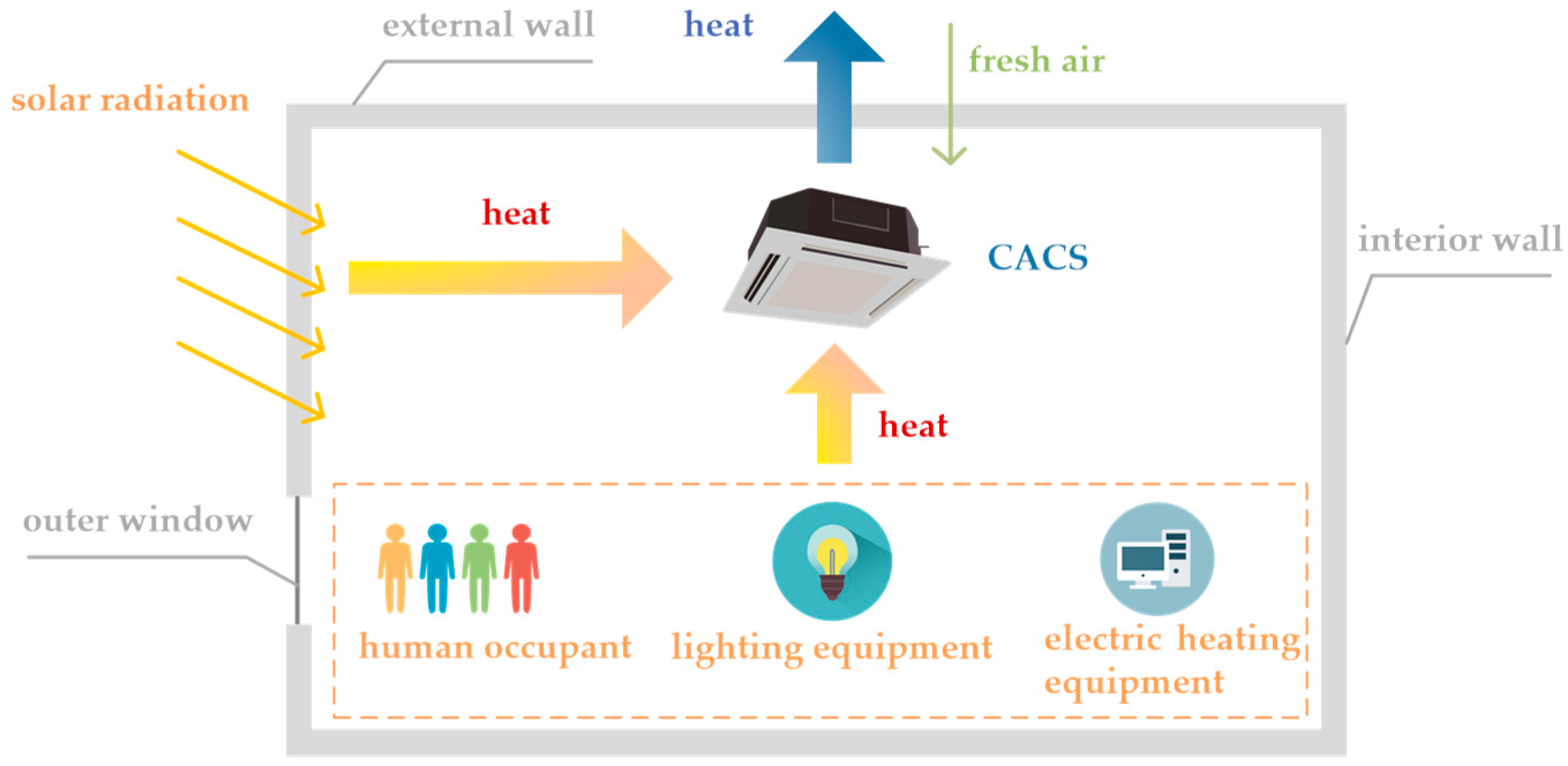
2. Central Air-Conditioning Systems

2.1. Comfort Index of the Human Body

A CACS is a kind of DR resource that can be beneficially regulated and controlled within a VPP setting to decrease the peak load of power grids and alleviate conflicts between power supply and demand. However, these systems must meet the comfort requirements of users. In this paper, the comfort requirements of users are determined using the predicted mean vote (PMV) index, denoted as ${\sigma }_{\mathrm{PMV}}$, which represents the thermal sensation registered by a majority of people within the same environment [35,36].

To ensure human comfort within an acceptable range, the present work applies the following constraint to the regulation and control processes of CACSs based on ${\sigma }_{\mathrm{PMV}}$ [37]:

$$–0.5\le {\sigma }_{\mathrm{PMV}}\le 0.5$$

(1)

The relationship between ${\sigma }_{\mathrm{PMV}}$ and the indoor temperature $T^{\mathrm{in}}$ can be expressed as follows [38,39]:

$${\sigma }_{\mathrm{PMV}}=\{\begin{array}{c}0.3895\times (T^{\mathrm{in}}-26),T^{\mathrm{in}}\ge 26\\ 0.4065\times (-T^{\mathrm{in}}+26),T^{\mathrm{in}}<26\end{array}$$

(2)

Therefore, the reasonable temperature range of human comfort can be determined according to Equations (1) and (2).

2.2. Central Air-Conditioning System Model

According to the principle of energy conservation, the heat obtained by a public building over a given period of time is the difference between the heat transferred in and the heat removed from the inside over that period [40]. A diagram of public building energy conservation is shown in Figure 2.

This yields the following thermodynamic equation in a public building with a CACS [41]:

$$\gamma \frac{\mathrm{d}{T}^{\mathrm{in}}}{\mathrm{d}t}+\beta T^{\mathrm{in}}-(\alpha -Q)=0$$

(3)

where $\alpha$, $\beta$, and $\gamma$ are parameters determined according to the individual characteristics of the public building and its CACS, and $Q$ is the total cold energy provided by the CACS. Accordingly, the time-varying equation of $T_t^{\mathrm{in}}$ can be obtained for a public building as follows [42]:

$$T_t^{\mathrm{in}}={\mathrm{e}}^{-\frac{\beta }{\gamma }\mathsf{\Delta }t}{T}_{t-1}^{\mathrm{in}}+(1-{\mathrm{e}}^{-\frac{\beta }{\gamma }\mathsf{\Delta }t})(\frac{{\alpha }_t}{\beta }-\frac{Q_t}{\beta })$$

(4)

$$\begin{array}{l}{\alpha }_t={\displaystyle \sum K_{\mathrm{wall}}}{A}_{\mathrm{wall}}(T_{\mathrm{cl}}+T_{\mathrm{d}})+{\displaystyle \sum q_{\mathrm{win}}}{A}_{\mathrm{win}}{F}_{\mathrm{d}}{F}_{\mathrm{s}}{F}_{\mathrm{cl}}+{\displaystyle \sum K_{\mathrm{win}}}{A}_{\mathrm{win}}{T}_t^{\mathrm{out}}+1000k_1{k}_2{k}_3{P}_{\mathrm{he}}+\\ 1000k_4{k}_5{k}_6{k}_7{P}_{\mathrm{le}}+C_{\mathrm{cl}}n\varphi q_{\mathrm{sh}}+n\varphi q_{\mathrm{lh}}+1.01G_{}^{\mathrm{n}}{T}_t^{\mathrm{out}}+38.5G_{}^{\mathrm{n}}\end{array}$$

(5)

$$\beta ={\displaystyle \sum K_{\mathrm{wall}}{A}_{\mathrm{wall}}+{\displaystyle \sum K_{\mathrm{win}}}}{A}_{\mathrm{win}}+1.01G_{}^{\mathrm{n}}$$

(6)

$$\gamma =C_{\mathrm{a}}V{\rho }_{\mathrm{a}}+S_{\mathrm{h}}{A}_{\mathrm{in}}$$

(7)

In addition, we present Equations (5)–(7) for determining the values of α, β, and γ for a public building. In terms of the external walls and roofs of the building, $K_{\mathrm{wall}}$, $A_{\mathrm{wall}}$, and $T_{\mathrm{cl}}$ are respectively the heat transfer coefficient, total area, and the hourly value of the cooling load temperature, and $T_{\mathrm{d}}$ is a correction value for $T_{\mathrm{cl}}$ with respect to the regions. In terms of the outer windows of the building, $q_{\mathrm{win}}$, $A_{\mathrm{win}}$, $F_{\mathrm{d}}$, $F_{\mathrm{s}}$, $F_{\mathrm{cl}}$, and $K_{\mathrm{win}}$ are respectively the maximum solar heat gain, total area, correction coefficient based on the glass type, shading coefficient associated with inner shading measures, cooling load coefficient, and heat transfer coefficient, and $T_t^{\mathrm{out}}$ is the outdoor temperature. In terms of the electric heating equipment of the building, $k_1$, $k_2$, $k_3$, and $P_{\mathrm{he}}$ are respectively the installation coefficient, load coefficient, simultaneous utilization rate, and installed power. In terms of the lighting equipment of the building, $k_4$, $k_5$, $k_6$, $k_7$, and $P_{\mathrm{le}}$ are respectively the simultaneous usage rate, heat storage coefficient, power consumption coefficient of rectifiers, installation coefficient, and installed power. In terms of the human occupants of the building, $C_{\mathrm{cl}}$ is the cooling load coefficient reflecting the sensible heat gain of a human body, $n$ is the total number of persons in the public building, $\varphi$ is the coefficient of occupant aggregation, $q_{\mathrm{sh}}$ is the sensible heat gain per adult male, $q_{\mathrm{lh}}$ is the latent heat gain per adult male, with all females and children converted into an adult male equivalence. Finally, $G_{}^{\mathrm{n}}$ is the fresh air volume of the building, $C_{\mathrm{a}}$ is the specific heat capacity of air at a constant pressure, $V_{}$ is the volume of refrigeration space in the building, ${\rho }_{\mathrm{a}}$ is the air density, $S_{\mathrm{h}}$ is the heat storage coefficient of interior walls, and $A_{\mathrm{in}}$ is the total area of interior walls.

A CACS is generally composed of chillers that produce cold energy $Q_t^{\mathrm{ch}}$ and thermal storage tanks for the storage and release of cold energy, which are denoted as $Q_t^{\mathrm{st}}$ and $Q_t^{\mathrm{re}}$, respectively. Accordingly, Q_t can be given as follows [39]:

$$Q_t=Q_t^{\mathrm{ch}}-Q_t^{\mathrm{st}}+Q_t^{\mathrm{re}}$$

(8)

The other constraints of a CACS can be expressed as follows:

$$0\le Q_t^{\mathrm{ch}}\le Q^{\mathrm{ch},\max }$$

(9)

$$0\le Q_t^{\mathrm{st}}\le Q^{\mathrm{st},\max }$$

(10)

$$0\le Q_t^{\mathrm{re}}\le Q^{\mathrm{re},\max }$$

(11)

$$0\le S_t^{\mathrm{c}}\le S^{\mathrm{c},\max }$$

(12)

$$S_t^{\mathrm{c}}=S_{t-1}^{\mathrm{c}}+(Q_t^{\mathrm{st}}{\eta }_{\mathrm{st}}-Q_t^{\mathrm{re}}/{\eta }_{\mathrm{re}})\mathsf{\Delta }t$$

(13)

Here, $Q^{\mathrm{ch},\max }$ is the maximum cold energy produced by chillers, $Q^{\mathrm{st},\max }$ and $Q^{\mathrm{re},\max }$ are the maximum cold energy respectively stored and released by thermal storage tanks, $S_t^{\mathrm{c}}$ and $S^{\mathrm{c},\max }$ are the respective cold energy in time period t and the cold energy capacity of thermal storage tanks, and ${\eta }_{\mathrm{st}}$ and ${\eta }_{\mathrm{re}}$ are the respective storage and release efficiencies of thermal storage tanks. Finally, the total power consumption of the CACS $P_t^{\mathrm{cold}}$ is mainly a function of the power consumed by chillers and the storage and release processes of thermal storage tanks, and can therefore be expressed as

$$P_t^{\mathrm{cold}}=Q_t^{\mathrm{ch}}/{\mu }_{\mathrm{ch}}+Q_t^{\mathrm{st}}{\mu }_{\mathrm{st}}+Q_t^{\mathrm{re}}{\mu }_{\mathrm{re}}$$

(14)

where ${\mu }_{\mathrm{ch}}$, ${\mu }_{\mathrm{st}}$, and ${\mu }_{\mathrm{re}}$ are the respective energy conversion efficiencies of chillers and of the storage and release processes of thermal storage tanks.

3. VPP Model Formulation

3.1. Deterministic VPP Model

The VPP model considered in the present work is composed of a PV power plant, a gas turbine power plant, an ESS, a CACS, and interruptible load. The VPP also participates in the DAM, RTM, and CTM simultaneously.

3.1.1. Objective Function

The optimization objective of the VPP owner is to maximize the cumulative profit, including the income obtained from participating in the DAM and RTM, the operation cost of the gas turbine $C_t^{\mathrm{GT}}$, the cost of interruptible load $C_t^{\mathrm{curt}}$, and the carbon trading cost $C^{\mathrm{c}}$ in the CTM. Therefore, the objective function can be expressed as:

$$\max {\displaystyle \sum _{t=1}^T({\lambda }_t^{\mathrm{DA}}(S_t^{\mathrm{DA}}-k^{\mathrm{p}}{P}_t^{\mathrm{DA}})+{\lambda }_t^{\mathrm{RT}}(S_t^{\mathrm{RT}}}-k^{\mathrm{p}}{P}_t^{\mathrm{RT}})-C_t^{\mathrm{GT}}-C_t^{\mathrm{curt}})-C^{\mathrm{c}}$$

(15)

where ${\lambda }_t^{\mathrm{DA}}$ and ${\lambda }_t^{\mathrm{RT}}$ are the respective electricity prices in the DAM and RTM, $P_t^{\mathrm{DA}}$ and $S_t^{\mathrm{DA}}$, and $P_t^{\mathrm{RT}}$ and $S_t^{\mathrm{RT}}$ are the volumes of electricity respectively purchased and sold in the DAM and RTM, respectively, and $k^{\mathrm{p}}$ is the coefficient of electricity purchase, which represents the ratio of purchasing price to selling price.

(1) Gas turbine operation cost

We modeled $C_t^{\mathrm{GT}}$ as the following piecewise linear approximation [43]:

$$C_t^{\mathrm{GT}}=a{u}_t^{\mathrm{GT}}+{\displaystyle \sum _{l=1}^{N_l}{K}_l{g}_{l,t}}+{\lambda }^{\mathrm{su}}{u}_t^{\mathrm{su}}+{\lambda }^{\mathrm{sd}}{u}_t^{\mathrm{sd}}$$

(16)

$$g_t^{\mathrm{GT}}={\displaystyle \sum _{l=1}^{N_l}{g}_{l,t}}$$

(17)

Here, $a$, ${\lambda }^{\mathrm{su}}$, and ${\lambda }^{\mathrm{sd}}$ are the respective fixed production, start-up, and shut-down costs of a gas turbine, $u_t^{\mathrm{GT}}$, $u_t^{\mathrm{su}}$, and $u_t^{\mathrm{sd}}$ are binary variables that respectively indicate whether the gas turbine is working, starting up, or shutting down, $K_l$ is the slope of the l-th segment of the gas turbine production cost curve composed of N_l segments, $g_{l,t}$ is the gas turbine production output in the l-th segment, and $g_t^{\mathrm{GT}}$ is the total power output of the gas turbine.

(2) Cost of interruptible load

Here, $C_t^{\mathrm{curt}}$ is the total compensation fees paid by the VPP to users when curtailing load demands. Different degrees of curtailment have different impacts on users according to the magnitude of the curtailment. Therefore, users are compensated for load curtailment according to the level of load curtailment. Accordingly, $C_t^{\mathrm{curt}}$ can be expressed as follows [44]:

$$C_t^{\mathrm{curt}}={\displaystyle \sum _{m=1}^{n_{\mathrm{m}}}({\lambda }_m^{\mathrm{curt}}{L}_{m,t}^{\mathrm{curt}})}$$

(18)

where $n_{\mathrm{m}}$ is the number of levels of load curtailment, ${\lambda }_m^{\mathrm{curt}}$ is the compensation price of the m-th level load curtailment, and $L_{m,t}^{\mathrm{curt}}$ is the magnitude of the m-th level load curtailment.

(3) Carbon trading cost

The carbon trading mechanism is based on a market-oriented adjustment mean that can effectively reduce the carbon emissions of the power industry and promote the development of energy saving and carbon emission reduction technologies. The Clean Development Mechanism is implemented as the carbon trading mechanism in this paper. First, this mechanism determines the carbon emission quota of each CTM participant over a period of time T, and monitors its carbon emission in real time. If the actual carbon emission of a participant is less than its quota, the remaining quota can be sold to the CTM for profit, while, when the actual carbon emission exceeds the quota, the insufficient quota must be purchased from the CTM or face a heavy fine [45].

Carbon emissions in a VPP mainly derive from the gas turbine, and can be expressed as:

$$E^{\mathrm{C}}={\displaystyle \sum _{t=1}^T\sigma g_t^{\mathrm{GT}}}$$

(19)

where $E^{\mathrm{C}}$ is the actual carbon emission of the VPP, and $\sigma$ is the carbon emission coefficient of the gas turbine. The carbon emission quota $E^{\mathrm{D}}$ of a VPP employed in the present work is based on the allocation scheme issued by the Shanghai Development and Reform Commission, which adopts the reference line method defined as follows [46]:

$$E^{\mathrm{D}}=\epsilon {\displaystyle \sum _{t=1}^T\eta P_t^{\mathrm{D}}}$$

(20)

where $\epsilon$ is the load rate correction factor, $\eta$ is the carbon emission quota per unit of electric power output, and $P_t^{\mathrm{D}}$ is the total power output of the VPP. Therefore, the value of $C^{\mathrm{c}}$ for a VPP can be expressed as:

$$C^{\mathrm{c}}={\lambda }^{\mathrm{c}}(E^{\mathrm{C}}-E^{\mathrm{D}})$$

(21)

where ${\lambda }^c$ is the carbon price in the CTM.

3.1.2. Constraints of Aggregated Units

(1) Gas turbine constraints [43]

$$u_t^{\mathrm{GT}}{g}^{\mathrm{GT},\min }\le g_t^{\mathrm{GT}}\le u_t^{\mathrm{GT}}{g}^{\mathrm{GT},\max }$$

(22)

$$-r^{\mathrm{D}}\le g_t^{\mathrm{GT}}-g_{t-1}^{\mathrm{GT}}\le r^{\mathrm{U}}$$

(23)

$$0\le g_{l,t}\le g_l^{\max }{u}_t^{\mathrm{GT}}$$

(24)

$$u_t^{\mathrm{GT}}-u_{t-1}^{\mathrm{GT}}\le u_t^{\mathrm{su}}$$

(25)

$$u_{t-1}^{\mathrm{GT}}-u_t^{\mathrm{GT}}\le u_t^{\mathrm{sd}}$$

(26)

$${\displaystyle \sum _{t=1}^{t^{\mathrm{sd}}-t^{\mathrm{sd},0}}{u}_t^{\mathrm{GT}}=0}$$

(27)

$${\displaystyle \sum _{t=1}^{t^{\mathrm{su}}-t^{\mathrm{su},0}}(1-u_t^{\mathrm{GT}})=0}$$

(28)

$$t^{\mathrm{su}}{u}_t^{\mathrm{su}}\le {\displaystyle \sum _{h=t}^{t+t^{\mathrm{su}}-1}{u}_t^{\mathrm{GT}}},\forall t\le T-t^{\mathrm{su}}+1$$

(29)

$$t^{\mathrm{sd}}{u}_t^{\mathrm{sd}}\le {\displaystyle \sum _{h=t}^{t+t^{\mathrm{sd}}-1}(1-u_t^{\mathrm{GT}})},\forall t\le T-t^{\mathrm{sd}}+1$$

(30)

Here, $g^{\mathrm{GT},\max }$ and $g^{\mathrm{GT},\min }$ are the respective maximum and minimum power outputs of the gas turbine, $r^{\mathrm{U}}$ and $r^{\mathrm{D}}$ are the respective ramp-up and ramp-down limits of the gas turbine, $g_l^{\max }$ is the capacity of the l-th segment of the gas turbine production cost curve, $t^{\mathrm{su}}$ and $t^{\mathrm{sd}}$ are the respective minimum up and down times, and $t^{\mathrm{su},0}$ and $t^{\mathrm{sd},0}$ are the respective initial up and down times.

(2) Energy storage system constraints [22]:

$$S_t^{\mathrm{es}}=S_{t-1}^{\mathrm{es}}+{\eta }_{\mathrm{c}}{g}_t^{\mathrm{esc}}-g_t^{\mathrm{esd}}/{\eta }_{\mathrm{d}}$$

(31)

$$S^{\mathrm{es},\min }\le S_t^{\mathrm{es}}\le S^{\mathrm{es},\max }$$

(32)

$$0\le g_t^{\mathrm{esc}}\le g^{\mathrm{esc},\max }$$

(33)

$$0\le g_t^{\mathrm{esd}}\le g^{\mathrm{esd},\max }$$

(34)

Here, $S_t^{\mathrm{es}}$ is the electrical energy stored in the ESS, ${\eta }_{\mathrm{c}}$ and ${\eta }_{\mathrm{d}}$ are the respective charge and discharge efficiencies of the ESS, $g_t^{\mathrm{esc}}$ and $g_t^{\mathrm{esd}}$ are the respective electrical charge and discharge power of the ESS, $S^{\mathrm{es},\max }$ and $S^{\mathrm{es},\min }$ are the respective maximum and minimum allowed electrical energy stored in the ESS, and $g^{\mathrm{esc},\max }$ and $g^{\mathrm{esd},\max }$ are the respective maximum electrical charge and discharge power of the ESS.

(3) Interruptible load constraints [15]

$$0\le L_{m,t}^{\mathrm{curt}}\le k_m^{\mathrm{curt}}{L}_t^{\mathrm{load}}$$

(35)

$$L_t^{\mathrm{curt}}={\displaystyle \sum _{m=1}^{n_{\mathrm{m}}}{L}_{m,t}^{\mathrm{curt}}}$$

(36)

$$L_{t-1}^{\mathrm{curt}}+L_t^{\mathrm{curt}}\le L^{\mathrm{curt},\max }$$

(37)

Here, $k_m^{\mathrm{curt}}$ is the load curtailment coefficient of the m-th level, $L_t^{\mathrm{load}}$ is the electrical load and $L_t^{\mathrm{curt}}$ is the magnitude of load curtailment in time period t, $L^{\mathrm{curt},\max }$ is the maximum magnitude of load curtailment in continuous time. Equation (37) avoids the decreased user satisfaction caused by an excessive magnitude of load curtailment in continuous time.

(4) Constraints of power sold to and purchased from the DAM and RTM [15]

$$0\le S_t^{\mathrm{DA}}\le S^{\mathrm{DA},\max }$$

(38)

$$0\le P_t^{\mathrm{DA}}\le P^{\mathrm{DA},\max }$$

(39)

$$0\le S_t^{\mathrm{RT}}\le S^{\mathrm{RT},\max }$$

(40)

$$0\le P_t^{\mathrm{RT}}\le P^{\mathrm{RT},\max }$$

(41)

Here, $P^{\mathrm{DA},\max }$ and $S^{\mathrm{DA},\max }$, and $P^{\mathrm{RT},\max }$ and $S^{\mathrm{RT},\max }$ are the respective maximum power sold to and purchased from the DAM and RTM, respectively.

(5) Energy balance constraint

$$S_t^{\mathrm{DA}}+S_t^{\mathrm{RT}}+g_t^{\mathrm{esc}}+L_t^{\mathrm{load}}-L_t^{\mathrm{curt}}+P_t^{\mathrm{cold}}=P_t^{\mathrm{DA}}+P_t^{\mathrm{RT}}+P_t^{\mathrm{RES}}+g_t^{\mathrm{GT}}+g_t^{\mathrm{esd}}$$

(42)

Here, $P_t^{\mathrm{RES}}$ is the power output of the PV power plant.

In addition, the deterministic model for the VPP must also meet constraints (1), (2), and (4)–(14) for the CACS.

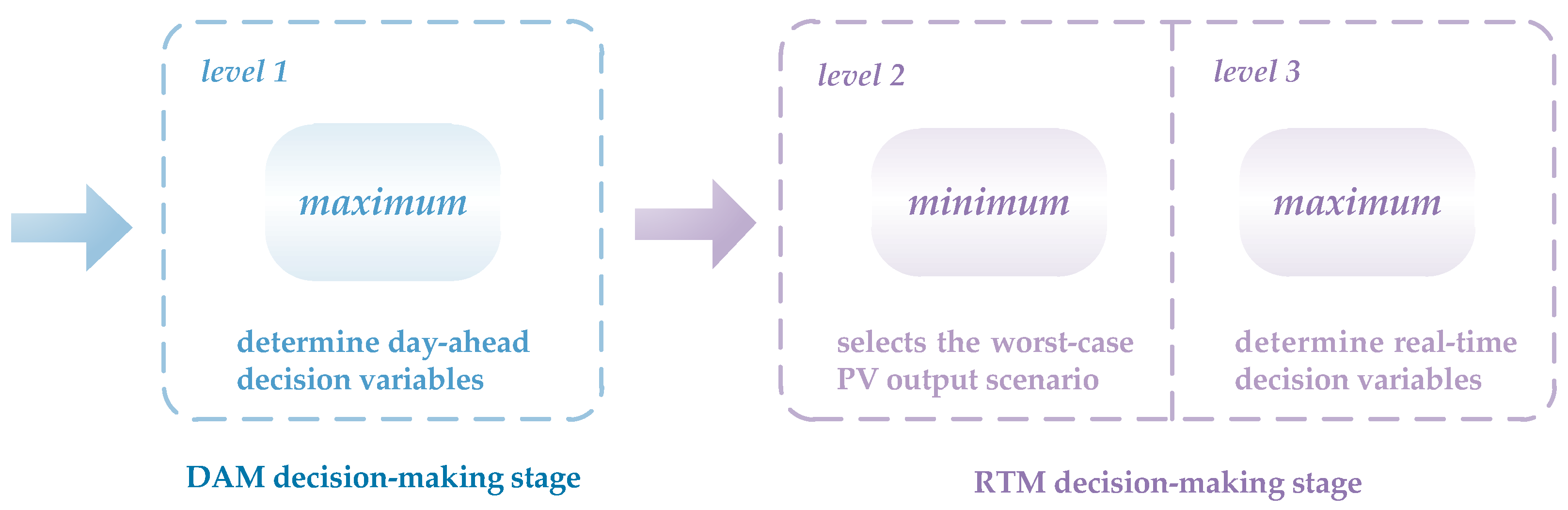
3.2. Stochastic Adaptive Robust Model for VPP Dispatch

The deterministic VPP model makes optimal scheduling decisions under the assumption that the market electricity price and PV output are known, while, in fact, both of these factors are uncertain to some degree. Therefore, the proposed stochastic adaptive robust VPP dispatch model combines the adaptive robust approach, which considers the worst-case PV output for addressing the relatively high level of PV output uncertainty, with the stochastic programming approach for addressing the relatively low level of market electricity price uncertainty [30].

The VPP model proposed in the present work is considered to participate in the DAM and RTM simultaneously. The day-ahead decision variables in the DAM stage are determined before the uncertain parameters of PV output are realized. In the RTM stage, the real-time decision variables are determined after the uncertain parameters of PV output and day-ahead decision variables are realized. Therefore, the proposed VPP model can adopt the form of a maximum-minimum-maximum process with a three-level structure that is composed of the following two stages:

• In the DAM decision-making stage (i.e., the pre-decision stage), the VPP determines the on/off statuses of the gas turbine and the DAM trading volume with the objective of maximizing profit.
• In the RTM decision-making stage (i.e., the re-decision stage), the VPP first considers the PV output of all scenarios on the basis of the realization of decision variables obtained at the DAM stage, and selects the worst-case scenario that minimizes the profit. Second, the VPP determines the RTM trading volume and other variables after the realization of the day-ahead decision variables and PV output with the objective of maximizing the profit.

The specific stochastic adaptive robust VPP dispatch model is accordingly given as follows in conjunction with the diagram shown in Figure 3.

(1) Objective function:

$$\max {\displaystyle \sum _{t=1}^T{\displaystyle \sum _{p=1}^{n_{\mathrm{p}}}\pi (p)}({\lambda }_{p,t}^{\mathrm{DA}}(S_{p,t}^{\mathrm{DA}}-k^{\mathrm{p}}{P}_{p,t}^{\mathrm{DA}}))}+\underset{P_s^{\mathrm{RES}}\in \mathsf{\Omega }}{\min }\max {\displaystyle \sum _{t=1}^T{\displaystyle \sum _{p=1}^{n_{\mathrm{p}}}\pi (p)}}({\lambda }_{p,t}^{\mathrm{RT}}(S_{p,t,s}^{\mathrm{RT}}-k^{\mathrm{p}}{P}_{p,t,s}^{\mathrm{RT}})-C_{p,t,s}^{\mathrm{GT}}-C_{p,t,s}^{\mathrm{curt}})-C_s^{\mathrm{c}}$$

(43)

Here, $n_{\mathrm{p}}$ is the total number of electricity price scenarios, $\pi (p)$ is the probability of the pth electricity price scenario, $p$ and $s$ are the respective electricity price and PV output scenarios, and $\mathsf{\Omega }$ is the original PV output scenario set.

(2) Day-ahead operation constraints:

$$u_{p,t}^{\mathrm{GT}}-u_{p,t-1}^{\mathrm{GT}}\le u_{p,t}^{\mathrm{su}}$$

(44)

$$u_{p,t-1}^{\mathrm{GT}}-u_{p,t}^{\mathrm{GT}}\le u_{p,t}^{\mathrm{sd}}$$

(45)

$${\displaystyle \sum _{t=1}^{t^{\mathrm{sd}}-t^{\mathrm{sd},0}}{u}_{p,t}^{\mathrm{GT}}=0}$$

(46)

$${\displaystyle \sum _{t=1}^{t^{\mathrm{su}}-t^{\mathrm{su},0}}(1-u_{p,t}^{\mathrm{GT}})=0}$$

(47)

$$t^{\mathrm{su}}{u}_{p,t}^{\mathrm{su}}\le {\displaystyle \sum _{h=t}^{t+t^{\mathrm{su}}-1}{u}_{p,t}^{\mathrm{GT}}},\forall t\le T-t^{\mathrm{su}}+1$$

(48)

$$t^{\mathrm{sd}}{u}_{p,t}^{\mathrm{sd}}\le {\displaystyle \sum _{h=t}^{t+t^{\mathrm{sd}}-1}(1-u_{p,t}^{\mathrm{GT}})},\forall t\le T-t^{\mathrm{sd}}+1$$

(49)

$$0\le S_{p,t}^{\mathrm{DA}}\le S^{\mathrm{DA},\max }$$

(50)

$$0\le P_{p,t}^{\mathrm{DA}}\le P^{\mathrm{DA},\max }$$

(51)

(3) Real-time operation constraints:

$$C_{p,t,s}^{\mathrm{GT}}=a{u}_{p,t}^{\mathrm{GT}}+{\displaystyle \sum _{l=1}^{N_l}{K}_l{g}_{l,p,t,s}}+{\lambda }^{\mathrm{su}}{u}_{p,t}^{\mathrm{su}}+{\lambda }^{\mathrm{sd}}{u}_{p,t}^{\mathrm{sd}}$$

(52)

$$g_{p,t,s}^{\mathrm{GT}}={\displaystyle \sum _{l=1}^{N_l}{g}_{l,p,t,s}}$$

(53)

$$u_{p,t}^{\mathrm{GT}}{g}^{\mathrm{GT},\min }\le g_{p,t,s}^{\mathrm{GT}}\le u_{p,t}^{\mathrm{GT}}{g}^{\mathrm{GT},\max }$$

(54)

$$-r^{\mathrm{D}}\le g_{p,t,s}^{\mathrm{GT}}-g_{p,t-1,s}^{\mathrm{GT}}\le r^{\mathrm{U}}$$

(55)

$$0\le g_{l,p,t,s}\le g_l^{\max }{u}_{p,t}^{\mathrm{GT}}$$

(56)

$$S_{p,t,s}^{\mathrm{es}}=S_{p,t-1,s}^{\mathrm{es}}+{\eta }_{\mathrm{c}}{g}_{p,t,s}^{\mathrm{esc}}-g_{p,t,s}^{\mathrm{esd}}/{\eta }_{\mathrm{d}}$$

(57)

$$S^{\mathrm{es},\min }\le S_{p,t,s}^{\mathrm{es}}\le S^{\mathrm{es},\max }$$

(58)

$$0\le g_{p,t,s}^{\mathrm{esc}}\le g^{\mathrm{esc},\max }$$

(59)

$$0\le g_{p,t,s}^{\mathrm{esd}}\le g^{\mathrm{esd},\max }$$

(60)

$$-0.5\le {\sigma }_{\mathrm{PMV}}\le 0.5$$

(61)

$${\sigma }_{\mathrm{PMV}}=\{\begin{array}{c}0.3895\times (T_{p,t,s}^{\mathrm{in}}-26),T_{p,t,s}^{\mathrm{in}}\ge 26\\ 0.4065\times (-T_{p,t,s}^{\mathrm{in}}+26),T_{p,t,s}^{\mathrm{in}}<26\end{array}$$

(62)

$$T_{p,t,s}^{\mathrm{in}}={\mathrm{e}}^{-\frac{\beta }{\gamma }\mathsf{\Delta }t}{T}_{p,t-1,s}^{\mathrm{in}}+(1-{\mathrm{e}}^{-\frac{\beta }{\gamma }\mathsf{\Delta }t})(\frac{{\alpha }_t}{\beta }-\frac{Q_{p,t,s}}{\beta })$$

(63)

$$Q_{p,t,s}=Q_{p,t,s}^{\mathrm{ch}}-Q_{p,t,s}^{\mathrm{st}}+Q_{p,t,s}^{\mathrm{re}}$$

(64)

$$0\le Q_{p,t,s}^{\mathrm{ch}}\le Q^{\mathrm{ch},\max }$$

(65)

$$0\le Q_{p,t,s}^{\mathrm{st}}\le Q^{\mathrm{st},\max }$$

(66)

$$0\le Q_{p,t,s}^{\mathrm{re}}\le Q^{\mathrm{re},\max }$$

(67)

$$0\le S_{p,t,s}^{\mathrm{c}}\le S^{\mathrm{c},\max }$$

(68)

$$S_{p,t,s}^{\mathrm{c}}=S_{p,t-1,s}^{\mathrm{c}}+(Q_{p,t,s}^{\mathrm{st}}{\eta }_{\mathrm{st}}-Q_{p,t,s}^{\mathrm{re}}/{\eta }_{\mathrm{re}})\mathsf{\Delta }t$$

(69)

$$P_{p,t,s}^{\mathrm{cold}}=Q_{p,t,s}^{\mathrm{ch}}/{\mu }_{\mathrm{ch}}+Q_{p,t,s}^{\mathrm{st}}{\mu }_{\mathrm{st}}+Q_{p,t,s}^{\mathrm{re}}{\mu }_{\mathrm{re}}$$

(70)

$$E_s^{\mathrm{D}}=\epsilon {\displaystyle \sum _{t=1}^T{\displaystyle \sum _{p=1}^{n_{\mathrm{p}}}\pi (p)}\eta P_{p,t,s}^{\mathrm{D}}}$$

(71)

$$E_s^{\mathrm{C}}={\displaystyle \sum _{t=1}^T{\displaystyle \sum _{p=1}^{n_{\mathrm{p}}}\pi (p)\sigma g_{p,t,s}^{\mathrm{GT}}}}$$

(72)

$$C_s^{\mathrm{c}}={\lambda }^{\mathrm{c}}(E_s^{\mathrm{C}}-E_s^{\mathrm{D}})$$

(73)

$$C_{p,t,s}^{\mathrm{curt}}={\displaystyle \sum _{m=1}^{n_{\mathrm{m}}}({\lambda }_m^{\mathrm{curt}}{L}_{m,p,t,s}^{\mathrm{curt}})}$$

(74)

$$0\le L_{m,p,t,s}^{\mathrm{curt}}\le k_m^{\mathrm{curt}}{L}_t^{\mathrm{load}}$$

(75)

$$L_{p,t,s}^{\mathrm{curt}}={\displaystyle \sum _{m=1}^{n_{\mathrm{m}}}{L}_{m,p,t,s}^{\mathrm{curt}}}$$

(76)

$$L_{p,t-1,s}^{\mathrm{curt}}+L_{p,t,s}^{\mathrm{curt}}\le L^{\mathrm{curt},\max }$$

(77)

$$0\le S_{p,t,s}^{\mathrm{RT}}\le S^{\mathrm{RT},\max }$$

(78)

$$0\le P_{p,t,s}^{\mathrm{RT}}\le P^{\mathrm{RT},\max }$$

(79)

$$S_{p,t}^{\mathrm{DA}}+S_{p,t,s}^{\mathrm{RT}}+g_{p,t,s}^{\mathrm{esc}}+L_t^{\mathrm{load}}-L_{p,t,s}^{\mathrm{curt}}+P_{p,t,s}^{\mathrm{cold}}=P_{p,t}^{\mathrm{DA}}+P_{p,t,s}^{\mathrm{RT}}+P_{t,s}^{\mathrm{RES}}+g_{p,t,s}^{\mathrm{GT}}+g_{p,t,s}^{\mathrm{esd}}$$

(80)

Compared with the deterministic model, the stochastic adaptive robust VPP dispatch model considers the electricity price scenarios in the DAM stage, and the day-ahead decision variables all include subscripts p and t. In the RTM stage, the electricity price and PV output scenarios are considered, and the real-time decision variables all contain subscripts p, t, and s.

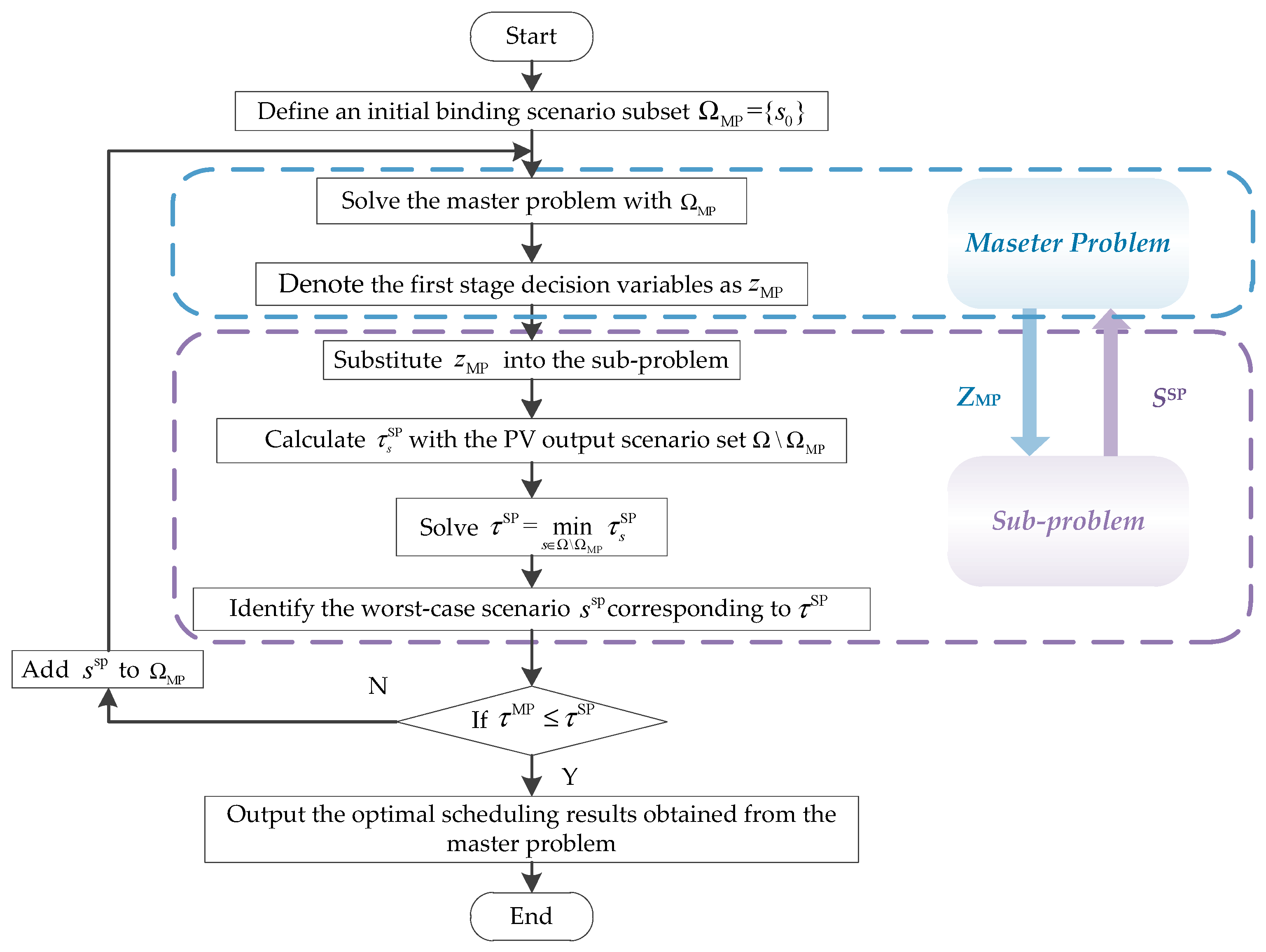
4. Binding Scenario Identification

The three-level adaptive robust VPP dispatch model is solved using the binding scenario identification approach. The solution algorithm decomposes the original model into a master problem and a sub-problem. The master problem in the first stage solves a single-level optimization model based on the binding scenario subset, and the sub-problem in the second stage solves a bi-level optimization model to identify the binding scenario subset [33]. Compared with the scenario-based algorithm [32], this approach greatly reduces the number of scenarios required for solution, alleviates the computational burden, and is adaptable to obtaining solutions of the adaptive robust model with large-scale scenario sets.

4.1. Master Problem

An auxiliary variable ${\tau }^{\mathrm{MP}}$ that represents the VPP profit obtained from the RTM in the worst case scenario $s^{\mathrm{SP}}$ is introduced to replace the minimum-maximum problem in the second stage of the stochastic adaptive robust VPP dispatch model. Therefore, this transforms the three-level optimization model of the original problem into the following single-level model for solution.

(1) Objective function:

$$\max {\displaystyle \sum _{t=1}^T{\displaystyle \sum _{p=1}^{n_{\mathrm{p}}}\pi (p)}({\lambda }_{p,t}^{\mathrm{DA}}(S_{p,t}^{\mathrm{DA}}-k^{\mathrm{p}}{P}_{p,t}^{\mathrm{DA}})})+{\tau }^{\mathrm{MP}}$$

(81)

$${\tau }^{\mathrm{MP}}\le {\displaystyle \sum _{t=1}^T{\displaystyle \sum _{p=1}^{n_{\mathrm{p}}}\pi (p)}({\lambda }_{p,t}^{\mathrm{RT}}(S_{p,t,s}^{\mathrm{RT}}-k^{\mathrm{p}}{P}_{p,t,s}^{\mathrm{RT}})}-C_{p,t,s}^{\mathrm{GT}}-C_{p,t,s}^{\mathrm{curt}})-C_s^{\mathrm{c}},\forall s\in {\mathsf{\Omega }}_{\mathrm{MP}}$$

(82)

(2) Day-ahead operation constraints: (44)–(51).

(3) Real-time operation constraints: (52)–(80), $\forall s\in {\mathsf{\Omega }}_{\mathrm{MP}}$.

Here, ${\mathsf{\Omega }}_{\mathrm{MP}}$ is the binding scenario subset.

The single-level optimization model of the master problem is considered to be equivalent to the three-level optimization model of the original problem when the master problem contains all vertices of the PV uncertainty set [32]. However, including all vertices of the PV uncertainty set will sharply increase the computational complexity of the solution process because each additional vertex will add a set of real-time operation constraints and variables in (52)–(80). Therefore, the original uncertainty set is replaced by the binding scenario subset ${\mathsf{\Omega }}_{\mathrm{MP}}$ that is identified in the sub-problem to reduce the number of scenarios and improve the computational efficiency of the solution process. Additionally, ${\mathsf{\Omega }}_{\mathrm{MP}}$ theoretically retains all essential information in the original uncertainty set, and therefore can guarantee that the single-level optimization model in the master problem is equivalent to the original three-level optimization model.

4.2. Sub-Problem

Firstly, an auxiliary variable ${\tau }_s^{\mathrm{SP}}$ is introduced to represent the VPP profit obtained from the RTM with the PV output scenario set $\mathsf{\Omega }\backslash {\mathsf{\Omega }}_{\mathrm{MP}}$. Here, $\mathsf{\Omega }\backslash {\mathsf{\Omega }}_{\mathrm{MP}}$ is the scenario set that ${\mathsf{\Omega }}_{\mathrm{MP}}$ is removing from $\mathsf{\Omega }$. Thus, the minimum-maximum model in the second stage of the original model is transformed into the following single-level model for solution.

(1) Objective function:

$$\max {\tau }_s^{\mathrm{SP}}={\displaystyle \sum _{t=1}^T{\displaystyle \sum _{p=1}^{n_{\mathrm{p}}}\pi (p)}({\lambda }_{p,t}^{\mathrm{RT}}(S_{p,t,s}^{\mathrm{RT}}-k^{\mathrm{p}}{P}_{p,t,s}^{\mathrm{RT}})-}{C}_{p,t,s}^{\mathrm{GT}}-C_{p,t,s}^{\mathrm{curt}})-C_s^{\mathrm{c}},\forall s\in \mathsf{\Omega }\backslash {\mathsf{\Omega }}_{\mathrm{MP}}$$

(83)

$${\tau }^{\mathrm{SP}}=\underset{s\in \mathsf{\Omega }\backslash {\mathsf{\Omega }}_{\mathrm{MP}}}{\min }{\tau }_s^{\mathrm{SP}}$$

(84)

(2) Real- time operation constraints: (52)–(80), $\forall s\in \mathsf{\Omega }\backslash {\mathsf{\Omega }}_{\mathrm{MP}}$.

Then, the value of ${\tau }_s^{\mathrm{SP}}$ obtained for each scenario of $\mathsf{\Omega }\backslash {\mathsf{\Omega }}_{\mathrm{MP}}$ is solved, and the worst-case scenario $s^{\mathrm{SP}}$ corresponding to the worst case VPP profit ${\tau }^{\mathrm{SP}}$ obtained in the sub-problem can be identified from Equation (84). However, the number of times the sub-problem must be solved increases as the size of the scenario set increases, resulting in low computational efficiency for relatively large scenario sets. Therefore, the auxiliary variable ${\tau }_{\mathrm{sum}}^{\mathrm{SP}}={\displaystyle \sum _{s\in \mathsf{\Omega }\backslash {\mathsf{\Omega }}_{\mathrm{MP}}}{\tau }_s^{\mathrm{SP}}}$ is introduced to replace the original cyclic solution process, and Equation (83) is converted into the following form:

$$\max {\tau }_{\mathrm{sum}}^{\mathrm{SP}}={\displaystyle \sum _{s\in \mathsf{\Omega }\backslash {\mathsf{\Omega }}_{\mathrm{MP}}}({\displaystyle \sum _{t=1}^T{\displaystyle \sum _{p=1}^{n_{\mathrm{p}}}\pi (p)}({\lambda }_{p,t}^{\mathrm{RT}}(S_{p,t,s}^{\mathrm{RT}}-}}{k}^{\mathrm{p}}{P}_{p,t,s}^{\mathrm{RT}})-C_{p,t,s}^{\mathrm{GT}}-C_{p,t,s}^{\mathrm{curt}})-C_s^{\mathrm{c}})$$

(85)

$${\tau }_s^{\mathrm{SP}}={\displaystyle \sum _{t=1}^T{\displaystyle \sum _{p=1}^{n_{\mathrm{p}}}\pi (p)}({\lambda }_{p,t}^{\mathrm{RT}}(S_{p,t,s}^{\mathrm{RT}}-k^{\mathrm{p}}{P}_{p,t,s}^{\mathrm{RT}})-}{C}_{p,t,s}^{\mathrm{GT}}-C_{p,t,s}^{\mathrm{curt}})-C_s^{\mathrm{c}},\forall s\in \mathsf{\Omega }\backslash {\mathsf{\Omega }}_{\mathrm{MP}}$$

(86)

Accordingly, $s^{\mathrm{SP}}$ can be identified by solving the sub-problem only once using Equations (85) and (86), which greatly improves the computational efficiency for relatively large scenario sets.

In the CCG algorithm, the KKT or duality method is used to transform the bi-level model (minimum-maximum model) of the sub-problem into a single-level model (maximum model) and inevitably introduces bilinear terms. Accordingly, the Big-M approach is used to linearize the nonlinear single-level model, which introduces a large number of integer terms and leads to high model solution complexity in large-scale problems. However, the use of auxiliary variables in the binding scenario identification algorithm employed in the present work avoids the introduction of bilinear and integer terms. In addition, the solution algorithm has the following advantages over the CCG algorithm:

• For nonlinear (nonconvex) problems, the optimality condition is false, which is not an appropriate condition for the CCG algorithm, while it is acceptable for the binding scenario identification algorithm.
• The scenario set used in the binding scenario identification algorithm to describe PV output uncertainty is more accurate than the box or polyhedron uncertainty set used in the CCG algorithm [47].
• The number of iterations required by the CCG algorithm depends on the coupling between each level of the problem, and may be quite large, while the number of iterations required by the binding scenario identification algorithm is limited because the number of binding scenarios is related to the uncertain scenario set and has nothing to do with the problem itself.

4.3. Solution Procedure

According to the previous discussion, the solution procedure for the binding scenario identification algorithm can be outlined as follows in conjunction with the specific algorithm flowchart shown in Figure 4:

• Define an initial binding scenario subset ${\mathsf{\Omega }}_{\mathrm{MP}}=\{s_0\}$, where $s_0$ is the initial PV output scenario.
• Solve the master problem with ${\mathsf{\Omega }}_{\mathrm{MP}}$, and denote the first stage decision variables {$S_{p,t}^{\mathrm{DA}\ast }$, $P_{p,t}^{\mathrm{DA}\ast }$, $u_{p,t}^{\mathrm{su}\ast }$, $u_{p,t}^{\mathrm{sd}\ast }$, $u_{p,t}^{\mathrm{GT}\ast }$} obtained from the master problem as $z_{\mathrm{MP}}$.
• Substitute $z_{\mathrm{MP}}$ into the sub-problem and calculate ${\tau }_s^{\mathrm{SP}}$ with the PV output scenario set $\mathsf{\Omega }\backslash {\mathsf{\Omega }}_{\mathrm{MP}}$. Solve ${\tau }^{\mathrm{SP}}=\underset{s\in \mathsf{\Omega }\backslash {\mathsf{\Omega }}_{\mathrm{MP}}}{\min }{\tau }_s^{\mathrm{SP}}$ to identify $s^{\mathrm{sp}}$.
• Compare ${\tau }^{\mathrm{MP}}$ obtained in the master problem with ${\tau }^{\mathrm{SP}}$ obtained in the sub-problem. If ${\tau }^{\mathrm{MP}}\le {\tau }^{\mathrm{SP}}$, ${\mathsf{\Omega }}_{\mathrm{MP}}$ includes the uncertainty information of all scenarios. Go to Step 5. Otherwise, add the scenario $s^{\mathrm{sp}}$ obtained to ${\mathsf{\Omega }}_{\mathrm{MP}}$, and go to Step 2.
• Output the optimal scheduling results obtained in Step 2.

5. Case Study

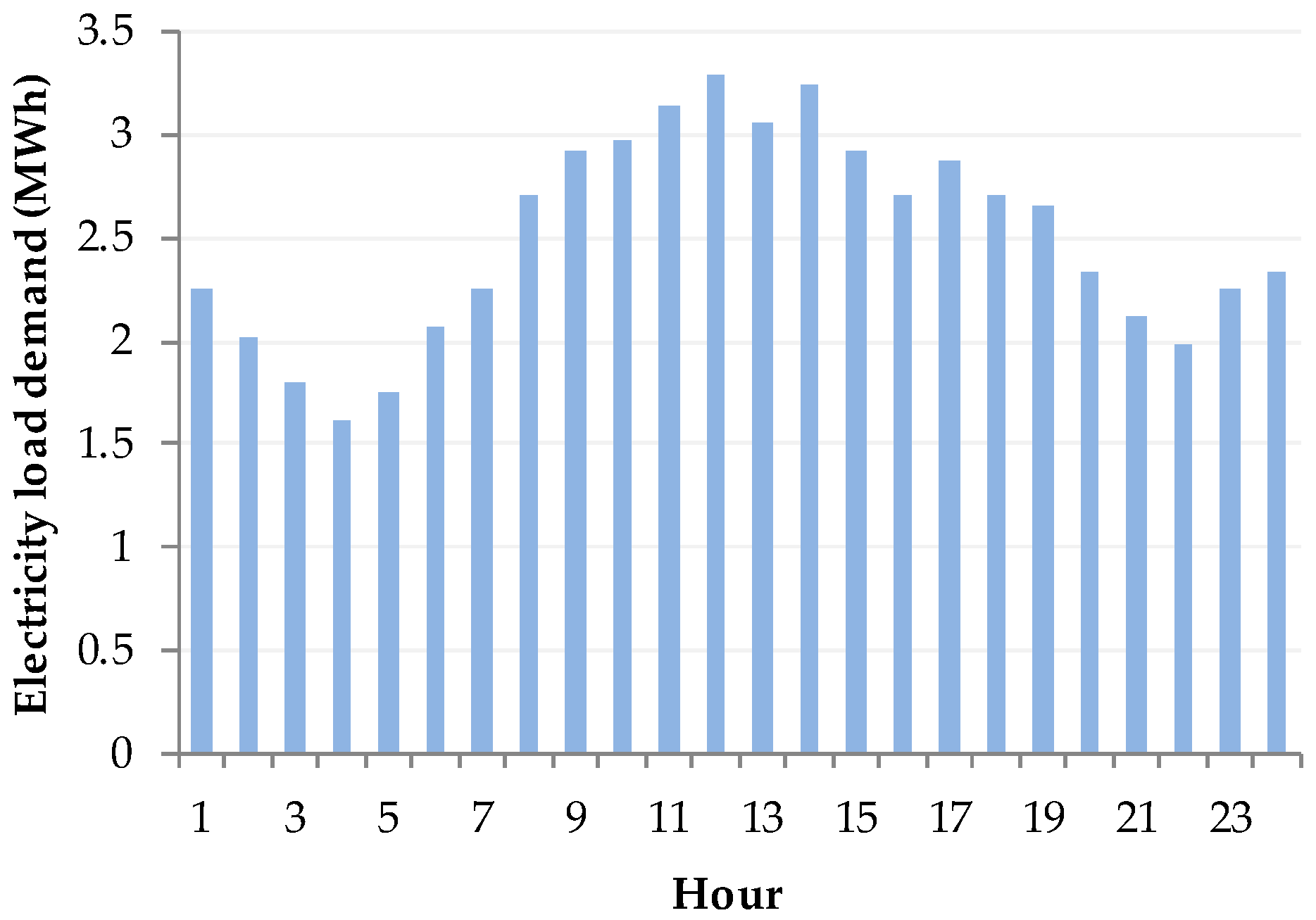
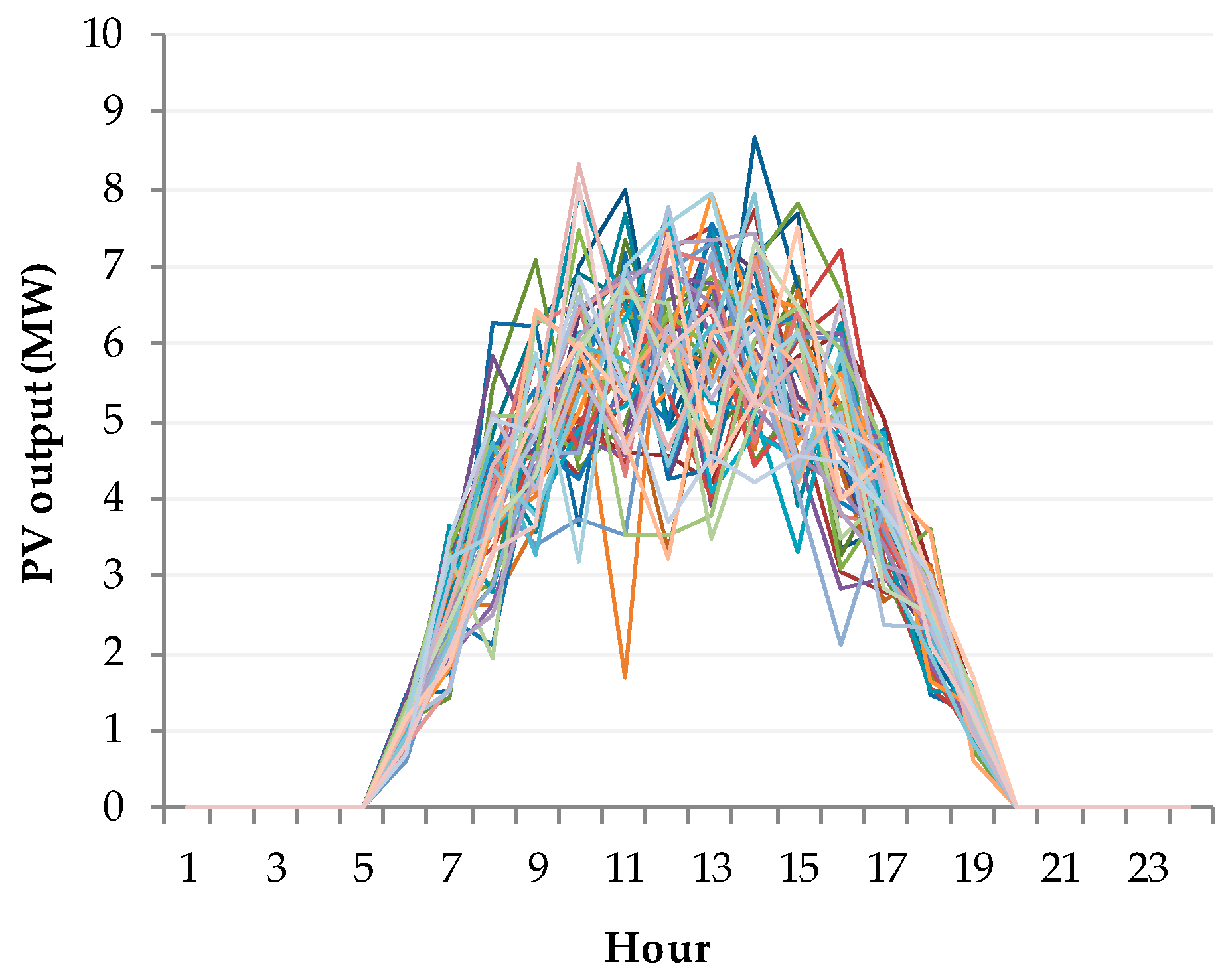
5.1. VPP Description and Parameter Settings

The VPP employed in this case study consists of a PV power plant, a TAU5670 gas turbine power plant, an ESS, a CACS in a public building, and interruptible load, and participates in the DAM, RTM, and CTM simultaneously. The scheduling cycle is set at 1 day and is divided into 24 periods of 1 h duration. The specific parameters of the aggregated units and the public building are listed in

Table A1. Parameters of the TAU5670 gas turbine.

Maximum/Minimum Output (MW)	Ramp-up/Ramp-down Limit (MW/h)	Start-up/Shut-down Cost (€)	Fixed Production Cost (€)
5.67/2.5	3/3	30/30	30
Slope of Segment l/2/3 (€/MW)	Minimum Up/Down Time (h)	Initial Up/Down Time (h)	Carbon Emission Coefficient/Quota (t/MWh)
40/45/50	2/2	0/1	0.184/0.3863

,

Table A2. Parameters of the CACS.

${\mathit{Q}}^{\mathbf{ch},\mathbf{max}}\left(\mathbf{MWh}\right)$	${\mathit{Q}}^{\mathbf{st},\mathbf{max}}\left(\mathbf{MWh}\right)$	${\mathit{Q}}^{\mathbf{re},\mathbf{max}}\left(\mathbf{MWh}\right)$	${\mathit{S}}^{\mathbf{c},\mathbf{max}}\left(\mathbf{MWh}\right)$	ηst	ηre	μch	μst	μre
10	5	5	26.4	0.95	0.92	5.6	0.008	0.007

,

Table A3. Parameters of the ESS.

${\mathit{g}}^{\mathbf{esc},\mathbf{max}}\left(\mathbf{MW}\right)$	${\mathit{g}}^{\mathbf{esd},\mathbf{max}}\left(\mathbf{MW}\right)$	${\mathit{S}}^{\mathbf{es},\mathbf{max}}\left(\mathbf{MWh}\right)$	ηc	ηd
8	8	40	0.9	0.9

and

Table A4. Parameters of the public building.

Type	Kwall,q * (W/(m2·K))	Kwall,d * (W/(m2·K))	Awall/Awin	(Tcl+Td)E ** (°C)	(Tcl+Td)S ** (°C)
Building	1.49	0.6	0.7/0.3	39	35.6
(Tcl+Td)W ** (°C)	(Tcl+Td)N ** (°C)	(Tcl+Td)H ** (°C)	Kwin(W/(m2·K))	qwin,E ** (W/m2)	qwin,W ** (W/m2)
39.4	34.9	37.6	5.8	531	531
qwin,S ** (W/m2)	qwin,N ** (W/m2)	Fcl,E **	Fcl,S **	Fcl,W **	Fcl,N **
195	145	0.31	0.81	0.24	0.85
Fd	Fs	k1	k2	k3	k4
0.93	1	0.7	0.7	1	0.85
k5	k6	k7	Sh(W/(m2·K))	Ccl	qsh(W)
1	1	0.7	10.63	0.03	63.94
qlh(W)	φ	Gn(m3/per·h)	n	Ple,ep *** (kW)	Ple,lp *** (kW)
117.46	0.89	10	3000	1280.13	1280.13
Phe,ep *** (kW)	Phe,lp *** (kW)	Ain,ep *** (m2)	Ain,lp *** (m2)	Ca(J/kg·°C)	ρa(kg /m3)
—	—	4704.7	4704.7	0.28	1.29

* Terms subscripted with q and d refer to the respective values obtained for external walls and roofs, respectively. ** Terms subscripted with E, S, W, N, and H refer to the respective values obtained in the east, south, west, north, and roof positions, respectively. *** Terms subscripted with ep and lp refer to the respective values obtained in the early and late peak-shaving periods, respectively.

of Appendix A. The length and width of the bottom side of the public building are 95 and 35 m, the story height is 4.7 m, and the number of floors is 11. The load demand over a single day is shown in Figure A1 of Appendix A. The interruptible load is divided into 3 levels, each of which is set at 10% of the total load. The curtailment compensation price of each level is respectively 40 €/MWh, 45 €/MWh, and 50 €/MWh. The carbon price is 6.569 €/t. Finally, Figure A2 and Figure A3 in Appendix A respectively present the five electricity price scenarios in the DAM and RTM and 50 PV power plant electricity output scenarios employed in the case study.

5.2. Simulation Results

The stochastic adaptive robust VPP dispatch model based on the binding scenario identification approach was jointly solved using GAMS and Matlab in this paper. All simulations were conducted on a personal computer equipped with an Intel Core 3.2 GHz CPU and 4 GB memory.

5.2.1. Analysis of the Factors Influencing VPP Profit

The impacts of DAM, RTM, and CTM participation and CACS regulation on VPP profit were analyzed according to the five schemes listed in

Table 1. Comparisons of VPP profit obtained under different conditions.

Scheme	Participate in DAM	Participate in RTM	Participate in CTM	Regulate Central Air-Conditioner	VPP Profit (€)
1	√	×	×	√	1104.63
2	√	×	√	√	1358.43
3	√	√	×	√	2925.01
4	√	√	√	×	3060.59
5	√	√	√	√	3199.39

along with the VPP profit obtained under each condition.

As shown in Table 1, the lowest VPP profit is obtained for Scheme 1 when the VPP participates in the DAM only, while the highest profit is obtained for Scheme 5 when the VPP participates in the DAM, RTM, and CTM simultaneously and the CACS is regulated by the VPP. We note from the results of Schemes 1 and 2 that the lack of participation in the RTM seriously detracts from VPP profitability because the VPP cannot select a suitable market to purchase/sell electricity by comparing the day-ahead price and real-time price. Similarly, Schemes 1 and 3 indicate that the lack of participation in the CTM also seriously detracts from VPP profitability because the carbon emission coefficient of the TAU5670 gas turbine is less than the carbon emission quota, and the PV power plant further reduces the carbon emissions of the units aggregated in the VPP. Therefore, the large surplus carbon emission quota cannot be sold to the CTM. Finally, a comparison of Schemes 4 and 5 indicates that CACS regulation by the VPP increases VPP profitability because the VPP can reduce cost by storing cold energy in low price periods and releasing cold energy in high price periods using the thermal storage tank.

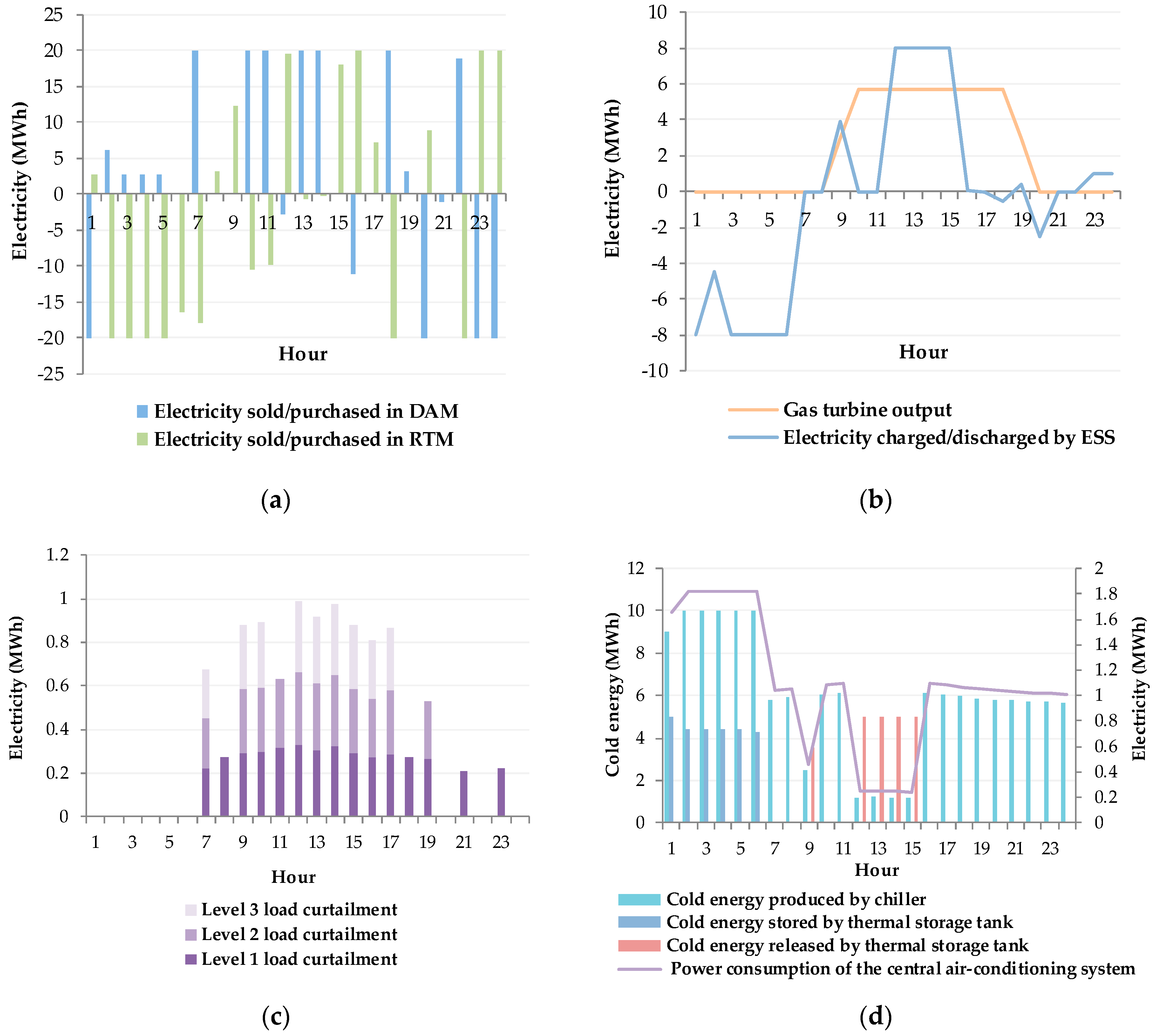
5.2.2. Analysis of Optimized VPP Dispatch Results

The optimized dispatch results obtained for the electricity sold/purchased by the VPP in the DAM and RTM and the aggregated units in the VPP over a 24 h period are shown in Figure 5.

The impact of purchasing and selling electricity by the VPP in the DAM and RTM has already been analyzed in Section 5.2.1; however, the actual purchasing and selling activities conducted by the VPP under Scheme 5 over the 24 h period are shown in Figure 5a. We note from Figure 5b that the gas turbine is started up when the electricity price is greater than the generation cost; otherwise, it is shut down. Similarly, the ESS charges during low price periods, and discharges during high price periods. The interruptible load dispatched at all levels is shown in Figure 5c. We note that the VPP can conduct partial load curtailment during high price periods and the load curtailment is conducted in the order of increasing levels according to the curtailment compensation price. Therefore, the VPP can increase its profitability by applying load curtailment to facilitate the selling of electricity within high price periods.

The dispatch results of the CACS are shown in Figure 5d. The cold energy produced by the chiller is at a maximum during hours 1–6 (low electricity price period), and the excess cold energy is stored in the thermal storage tank. The cold energy stored in the thermal storage tank has reached its upper limit at hour 7 or 8, so the chiller is limited to meeting the indoor temperature requirements only, which accordingly decreases the chiller output. During high electricity price periods, the CACS takes advantage of the fact that the power consumption of the thermal storage tank is much less than that of the chiller, and elects to release cold energy from the thermal storage tank, while the additional cooling is provided by the chiller. Finally, the thermal storage tank stops working during the hours of 16–24 because the profit obtained by transferring the period of high power consumption by the CACS according to the difference between peak and valley electricity prices is not sufficient to make up for the loss associated with the storage/release process. These results demonstrate that the cold energy storage and release function of the thermal storage tank facilitates the concentration of power consumption by the CACS during low electricity price periods, which not only reduces the cost of the VPP, but can also alleviate the problems associated with peak load periods via load shifting.

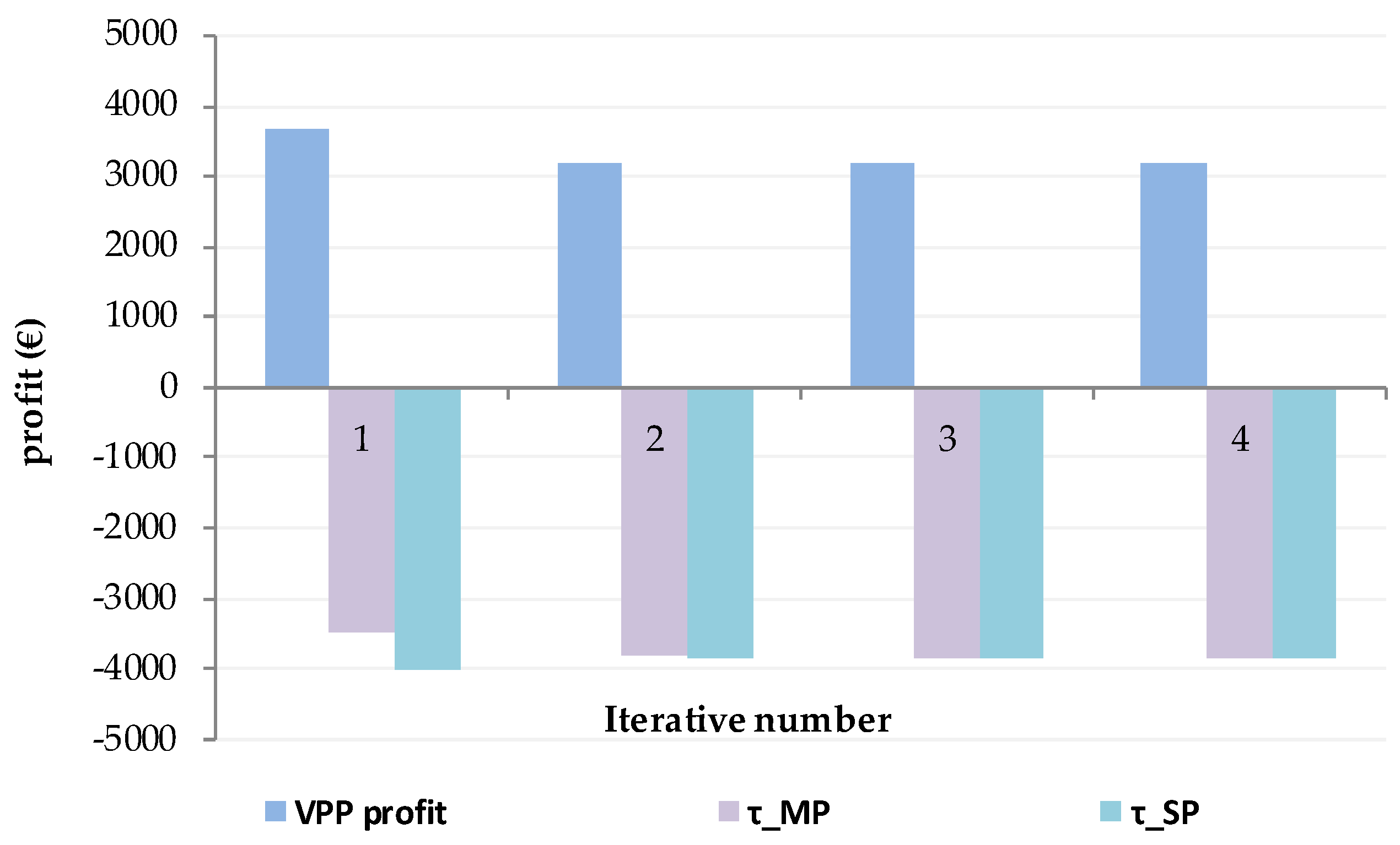
5.2.3. Analysis of Iteration Performance

The VPP profit results and values for the auxiliary variables ${\tau }^{\mathrm{MP}}$ and ${\tau }^{\mathrm{SP}}$ obtained for each iteration of the solution algorithm based on the binding scenario identification approach are shown in Figure 6. The results indicate that the VPP profit consistently decreases. This is because the sub-problem identifies a binding scenario from the PV scenario set after each iteration, and the master problem must apply a set of real-time operation constraints and variables, so that the constraints on the master problem are progressively enhanced. The VPP profit decreases greatly from 3682.23 € to 3208.92 € in the second iteration and stabilizes gradually as the number of iterations increases. Similarly, the difference between ${\tau }^{\mathrm{MP}}$ and ${\tau }^{\mathrm{SP}}$ substantially decreases in the second iteration, and gradually stabilizes with increasing iterations. Accordingly, the binding scenario identification approach obtains the optimal scheduling result in 4 iterations. This is because the binding scenario subset of the master problem contains the worst-case scenario of all scenarios in the second iteration, and the severity of the worst-case scenarios identified by the sub-problem decreases in subsequent iterations.

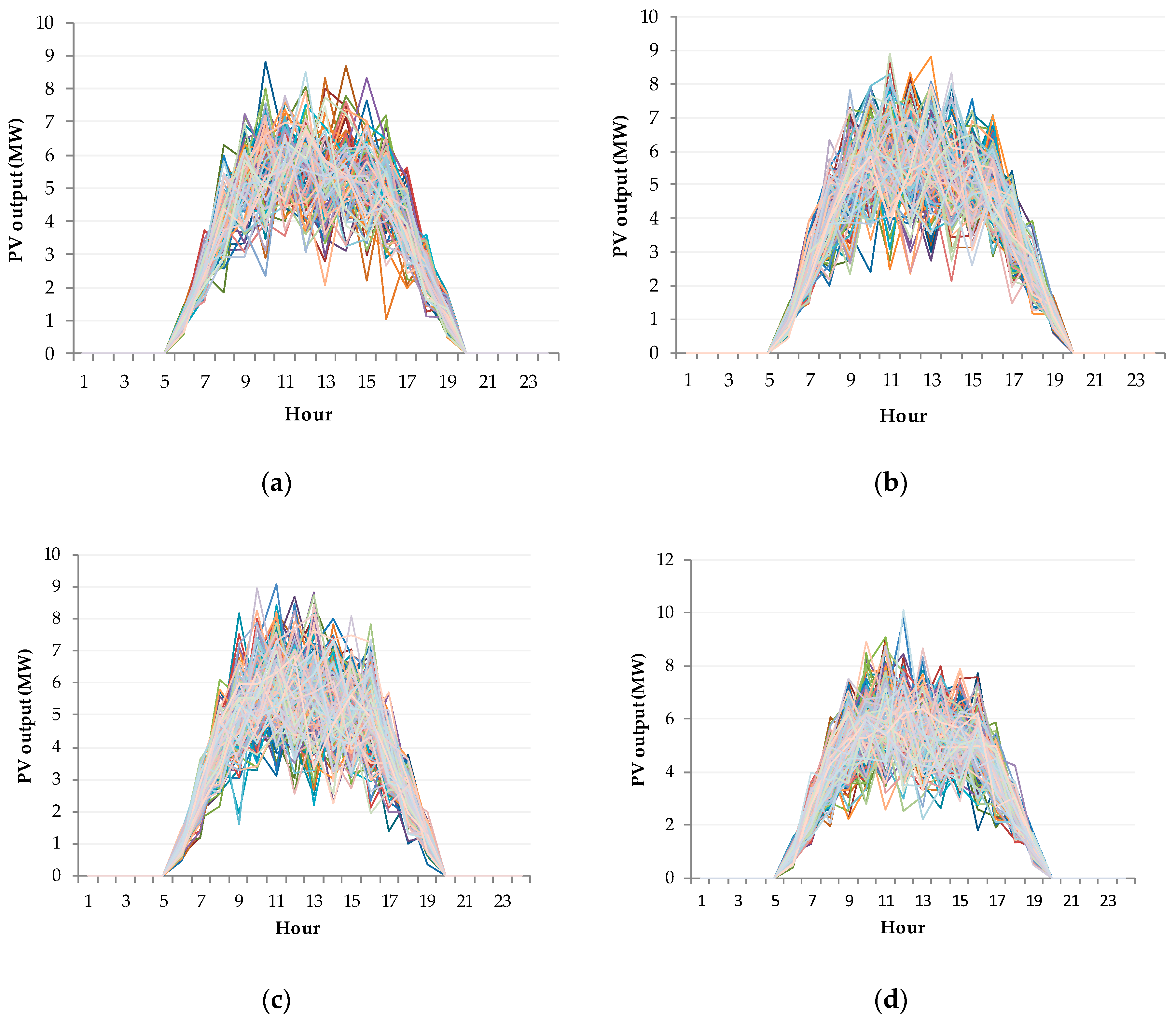
5.2.4. Analysis of Adaptability to Large-scale Scenario Sets

The adaptability of the binding scenario identification algorithm to large-scale scenario sets is demonstrated by comparing the computation times and numbers of iterations required to solve Case 1 with the 50 PV power output scenarios shown in Figure A3, with those required to solve Cases 2–5 shown in Figure A4 of Appendix A, which involve 100, 150, 200, and 250 PV power output scenarios, respectively. The results are shown in Figure 7.

As can be seen from Figure 7, the number of iterations required by the binding scenario identification approach is basically constant for all cases, and only 3 or 4 iterations are needed to achieve convergence. Consequently, only 3 or 4 binding scenarios are identified by the sub-problem in each case because the sub-problem identifies a single binding scenario in each iteration. The computation time required for each binding scenario identification of the sub-problem increases with an increasing number of scenarios in the scenario set while the number of times the master problem and sub-problem required to be solved basically remains unchanged. Therefore, the computation time of the binding scenario identification approach increases only slowly with an increasing number of scenarios in the scenario set, as shown in Figure 7. These results demonstrate that the identification of the binding scenario subset in the sub-problem greatly reduces the required number of scenarios, and thereby substantially increases the computational efficiency of the solution algorithm. Accordingly, the binding scenario identification algorithm can readily adapt to the stochastic adaptive robust VPP dispatch model with large-scale scenario sets.

5.2.5. Comparative Analysis of the Binding Scenario Identification Approach

As discussed, the standard scenario-based approach [32] employs the entire scenario set, and therefore cannot fail to obtain an optimum scheduling result. However, in so doing, it suffers from a high computational burden. Therefore, we compare the solution results obtained for Cases 1–5 using the binding scenario identification approach and the standard scenario-based algorithm approach for the stochastic adaptive robust VPP dispatch model in

Table 2. Comparison of the solutions obtained using the binding scenario identification approach and the standard scenario-based approach [32] for the stochastic adaptive robust VPP dispatch model.

Optimized Results	Case 1	Case 2	Case 3	Case 4	Case 5
Number of scenarios	50	100	150	200	250
Number of iterations	4	3	3	3	3
Binding scenariosubsets	1/23/49/37	1/12/9	1/110/32	1/41/186	1/171/14
VPP profit of binding scenario approach (€)	3199.4	2932.4	2862.3	2836.6	2929.7
VPP profit of standard scenario-based approach (€)	3199.4	2932.4	2862.3	2836.6	2929.7
Auxiliary variable${\tau }^{\mathrm{MP}}$of binding scenario approach (€)	−3848.1	−3848.1	−4021.1	−3954.9	−3951.6
Auxiliary variable${\tau }^{\mathrm{MP}}$of standard scenario-based approach (€)	−3848.1	−3848.1	−4021.1	−3954.9	−3951.6

. In addition, the efficiencies of the two algorithms are compared in Figure 8.

As is shown in Table 2, the VPP profit and ${\tau }^{\mathrm{MP}}$ values obtained by the two algorithms are equivalent for all Cases 1–5. These results demonstrate that the subset identified by the binding scenario identification approach can accurately replace the initial PV output scenario set, that is, the non-binding scenarios have no effect on the optimization results. Therefore, the binding scenario identification approach provides an equivalent solution accuracy as that obtained by the standard scenario-based approach. In terms of algorithm efficiency, Figure 8 demonstrates that the computation time of the standard scenario-based approach increases sharply with an increasing number of scenarios. In fact, the stochastic adaptive robust VPP dispatch model may even be unsolvable by the standard scenario-based approach for a sufficiently large-scale scenario set, as shown in

Table A5. Comparison of the computation times of the two algorithms in Cases 6–10.

Optimized Results	Case 6	Case 7	Case 8	Case 9	Case 10
Number of scenarios	400	500	600	700	800
Computation time of binding scenario approach(s)	66.56	86.63	110.34	133.67	165.48
Computation timeof standard scenario-based approach(s)	421.44	882.88	1049	Unsolvable	Unsolvable

of Appendix A. In contrast, the required computation time of the binding scenario identification approach increases much more slowly with an increasing number of scenarios, indicating that the computational efficiency is much greater than that of the standard scenario-based approach, particularly with large-scale scenario sets.

6. Conclusions

This paper established a stochastic adaptive robust dispatch model for a VPP that aggregates a PV power plant, a gas turbine power plant, an ESS, a CACS, and interruptible load while considering VPP participation in the DAM, RTM, and CTM simultaneously and uncertainties in the electricity market price and PV generation output. The stochastic programming approach was adopted for addressing the uncertainty in electricity market price, and the adaptive robust approach was adopted for addressing the uncertainty in PV generation output. The model was decomposed into a master problem and a sub-problem using the binding scenario identification approach. The master problem was used to solve the single-level optimization model with the binding scenario subset, and the sub-problem was used to identify the binding scenario subset. Finally, the validity of the model and algorithm was verified by a case study with varying numbers of PV generation output scenarios. The primary conclusions can be summarized as follows:

• Simultaneous participation in the DAM, RTM, and CTM allows the VPP to dispatch flexibly according to the electricity market price, which improves the profitability of the VPP and adapts its functionality to emerging low carbon emission requirements.
• The VPP can conduct the coordinated scheduling of aggregated units, such as the interruptible load and CACS, to reduce electricity consumption during high electricity price periods and alleviate problems associated with peak loads via load shifting.
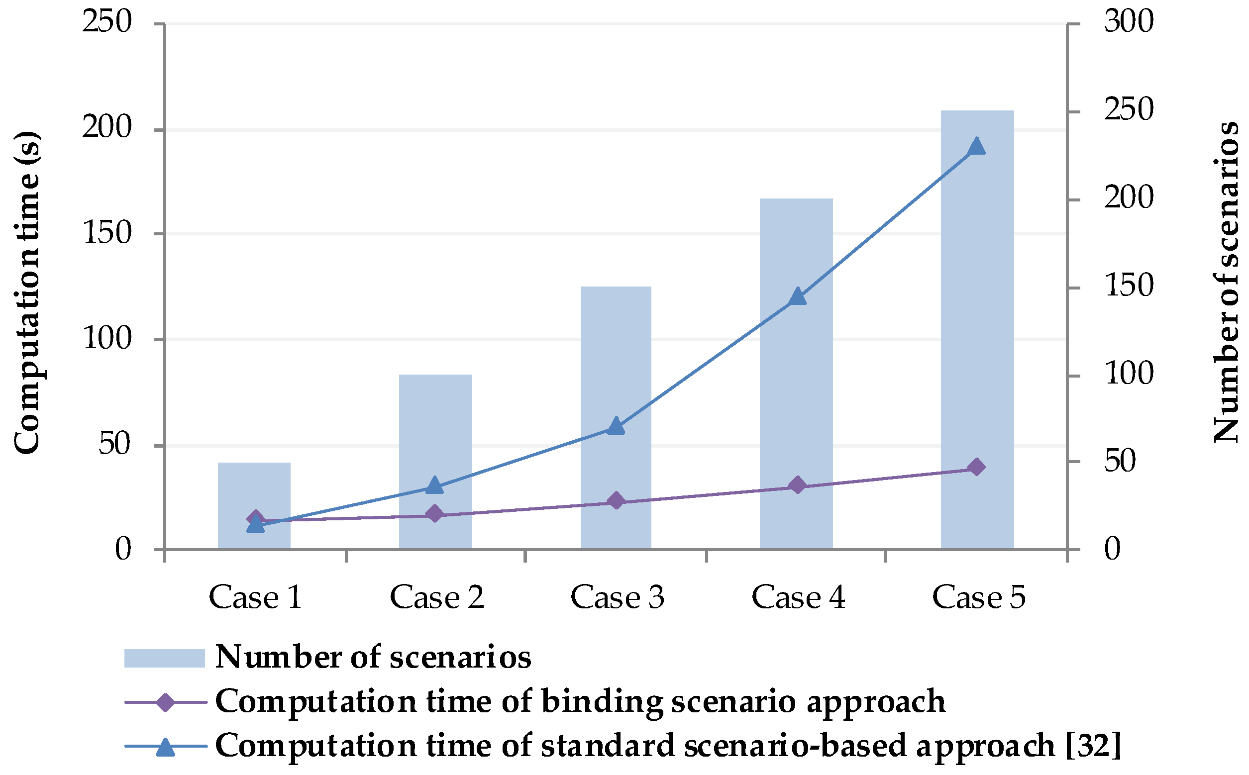
• The binding scenario identification approach greatly reduces the number of scenarios that must be considered, and thereby increases the computational efficiency of the solution algorithm. The required computation time increases slowly with increasing size of the scenario set, so that the solution algorithm is adaptable to the stochastic adaptive robust VPP dispatch model with large-scale scenario sets.
• The binding scenario identification approach accurately identifies the binding scenario subset, and therefore attains an equivalent solution accuracy as that of the standard scenario-based approach, while providing a greatly increased computational efficiency.

Future works will focus on two major parts: firstly, the effects of CACS modeling parameters on VPP profit will be studied. Secondly, the stochastic adaptive robust model for VPP dispatch and binding scenario identification approach will be tested using more real market scenarios.

References

1. Pourakbari-Kasmaei, M.; Mantovani, J.R.S.; Rashidinejad, M.; Habibi, M.R.; Contreras, J. Carbon footprint allocation among consumers and transmission losses. In Proceedings of the 2017 IEEE International Conference Environment and Electrical Engineering and 2017 IEEE Industrial and Commercial Power Systems Europe (EEEIC/I&CPS Europe), Milan, Italy, 6–9 June 2017. [Google Scholar]
2. Tofis, Y.; Yiasemi, Y.; Kyriakides, E. A plug-and-play selective load shedding scheme for power systems. IEEE Syst. J. 2017, 11, 2864–2871. [Google Scholar] [CrossRef]
3. Li, H.; Eseye, A.T.; Zhang, J.; Zheng, D. Optimal energy management for industrial microgrids with high-penetration renewables. Prot. Control Mod. Power Syst. 2017, 2, 12. [Google Scholar] [CrossRef]
4. Wang, J.; Yang, W.; Cheng, H.; Huang, L.; Gao, Y. The Optimal Configuration Scheme of the Virtual Power Plant Considering Benefits and Risks. Energies 2017, 10, 968. [Google Scholar] [CrossRef]
5. Li, J.; Wang, S.; Ye, L.; Fang, J. A coordinated dispatch method with pumped-storge and battery-storage for compensating the variation of wind power. Prot. Control Mod. Power Syst. 2018, 3, 2. [Google Scholar] [CrossRef]
6. Zang, H.; Cheng, L.; Ding, T.; Cheung, K.W.; Liang, Z.; Wei, Z.; Sun, G. Hybrid method for short-term photovoltaic power forecasting based on deep convolutional neural network. IET Gener. Transm. Distrib. 2018, 12, 4557–4567. [Google Scholar] [CrossRef]
7. Magdy, G.; Mohamed, E.A.; Shabib, G.; Elbaset, A.A.; Mitani, Y. Microgrid dynamic security considering high penetration of renewable energy. Prot. Control Mod. Power Syst. 2018, 3, 23. [Google Scholar] [CrossRef]
8. Bashir, A.A.; Pourakbari-Kasmaei, M.; Contreras, J.; Lehtonen, M. A novel energy scheduling framework for reliable and economic operation of islanded and grid-connected microgrids. Electr. Power Syst. Res. 2019, 171, 85–96. [Google Scholar] [CrossRef]
9. Luo, J.; Cao, Y.; Yang, W.; Yang, Y.; Zhao, Z.; Tian, S. Optimal Operation Modes of Virtual Power Plants Based on Typical Scenarios Considering Output Evaluation Criteria. Energies 2018, 11, 2634. [Google Scholar] [CrossRef]
10. Home-Ortiz, J.M.; Pourakbari-Kasmaei, M.; Lehtonen, M.; Mantovani, J.R.S. Optimal location-allocation of storage devices and renewable-based DG in distribution systems. Electr. Power Syst. Res. 2019, 172, 11–21. [Google Scholar] [CrossRef]
11. Qiu, J.; Zhao, J.; Wang, D.; Zheng, Y. Two-stage coordinated operational strategy for distributed energy resources considering wind power curtailment penalty cost. Energies 2017, 10, 965. [Google Scholar] [CrossRef]
12. Rahimiyan, M.; Baringo, L. Strategic bidding for a virtual power plant in the day-ahead and real-time markets: Price-taker robust optimization approach. IEEE Trans. Power Syst. 2016, 31, 2676–2687. [Google Scholar] [CrossRef]
13. Wang, Y.; Ai, X.; Tan, Z.; Yan, L.; Liu, S. Interactive dispatch modes and bidding strategy of multiple virtual power plants based on demand response and game theory. IEEE Trans. Smart Grid 2015, 7, 510–519. [Google Scholar] [CrossRef]
14. Pazouki, S.; Haghifam, M.R.; Pazouki, S. Transition from fossil fuels power plants toward Virtual Power Plants of distribution networks. In Proceedings of the 2016 21st Conference on Electrical Power Distribution Networks Conference (EPDC), Karaj, Iran, 26–27 April 2016. [Google Scholar]
15. Liang, Z.; Alsafasfeh, Q.; Jin, T.; Pourbabak, H.; Su, W. Risk-constrained optimal energy management for virtual power plants considering correlated demand response. IEEE Trans. Smart Grid 2017, 10, 1577–1587. [Google Scholar] [CrossRef]
16. Al-Awami, A.T.; Amleh, N.; Muqbel, A. Optimal demand response bidding and pricing mechanism with fuzzy optimization: Application for a virtual power plant. IEEE Trans. Ind. Appl. 2017, 53, 5051–5061. [Google Scholar] [CrossRef]
17. Kardakos, E.G.; Simoglou, C.K.; Bakirtzis, A.G. Optimal offering strategy of a virtual power plant: A stochastic bi-level approach. IEEE Tran. Smart Grid 2015, 7, 794–806. [Google Scholar] [CrossRef]
18. Gao, Y.; Xue, F.; Yang, W.; Yang, Q.; Sun, Y.; Sun, Y.; Liang, H.; Li, P. Optimal operation models of photovoltaic-battery energy storage system based power plants considering typical scenarios. Prot. Control Mod. Power Syst. 2017, 2, 397–406. [Google Scholar] [CrossRef]
19. Pandžić, H.; Kuzle, I.; Capuder, T. Virtual power plant mid-term dispatch optimization. Appl. Energy 2013, 101, 134–141. [Google Scholar] [CrossRef]
20. Ding, H.; Hu, Z.; Song, Y. Stochastic optimization of the daily operation of wind farm and pumped-hydro-storage plant. Renew. Energy 2012, 48, 571–578. [Google Scholar] [CrossRef]
21. Dabbagh, S.R.; Sheikh-El-Eslami, M.K. Risk assessment of virtual power plants offering in energy and reserve markets. IEEE Trans. Power Syst. 2015, 31, 3572–3582. [Google Scholar] [CrossRef]
22. Zhou, Y.; Wei, Z.; Sun, G.; Cheung, K.W.; Zang, H.; Chen, S. A robust optimization approach for integrated community energy system in energy and ancillary service markets. Energy 2018, 148, 1–15. [Google Scholar] [CrossRef]
23. Ju, L.; Li, H.; Zhao, J.; Chen, K.; Tan, Q.; Tan, Z. Multi-objective stochastic scheduling optimization model for connecting a virtual power plant to wind-photovoltaic-electric vehicles considering uncertainties and demand response. Energy Conv. Manag. 2016, 128, 160–177. [Google Scholar] [CrossRef]
24. Shayegan-Rad, A.; Badri, A.; Zangeneh, A. Day-ahead scheduling of virtual power plant in joint energy and regulation reserve markets under uncertainties. Energy 2017, 121, 114–125. [Google Scholar] [CrossRef]
25. Zhao, C.; Guan, Y. Unified stochastic and robust unit commitment. IEEE Trans. Power Syst. 2013, 28, 3353–3361. [Google Scholar] [CrossRef]
26. An, Y.; Zeng, B. Exploring the modeling capacity of two-stage robust optimization: Variants of robust unit commitment model. IEEE Trans. Power Syst. 2015, 30, 109–122. [Google Scholar] [CrossRef]
27. Jiang, R.; Wang, J.; Guan, Y. Robust unit commitment with wind power and pumped storage hydro. IEEE Trans. Power Syst. 2012, 27, 800–810. [Google Scholar] [CrossRef]
28. Ding, T.; Liu, S.; Yuan, W.; Bie, Z.; Zeng, B. A two-stage robust reactive power optimization considering uncertain wind power integration in active distribution networks. IEEE Trans. Sustain. Energy 2016, 7, 301–311. [Google Scholar] [CrossRef]
29. Bertsimas, D.; Brown, D.B.; Caramanis, C. Theory and applications of robust optimization. Siam Rev. 2011, 53, 464–501. [Google Scholar] [CrossRef]
30. Baringo, A.; Baringo, L. A stochastic adaptive robust optimization approach for the offering strategy of a virtual power plant. IEEE Trans. Power Syst. 2017, 32, 3492–3504. [Google Scholar] [CrossRef]
31. Charwand, M.; Ahmadi, A.; Heidari, A.R.; Nezhad, A.E. Benders decomposition and normal boundary intersection method for multiobjective decision making framework for an electricity retailer in energy markets. IEEE Syst. J. 2015, 9, 1475–1484. [Google Scholar] [CrossRef]
32. Morales, J.M.; Conejo, A.J.; Madsen, H.; Pinson, P.; Zugno, M. Integrating Renewables in Electricity Markets: Operational Problems, 1st ed.; Springer: Berlin, Germany, 2014; pp. 57–91. [Google Scholar]
33. Chen, S.; Wei, Z.; Sun, G.; Cheung, K.W.; Wang, D.; Zang, H. Adaptive Robust Day-Ahead Dispatch for Urban Energy Systems. IEEE Trans. Ind. Electron. 2019, 66, 1379–1390. [Google Scholar] [CrossRef]
34. Soares, T.; Bessa, R.J.; Pinson, P.; Morais, H. Active distribution grid management based on robust ac optimal power flow. IEEE Trans. Smart Grid 2017, 9, 6229–6241. [Google Scholar] [CrossRef]
35. Nian, F.; Wang, K. Study on indoor environmental comfort based on improved PMV index. In Proceedings of the 2017 3rd International Conference on Computational Intelligence & Communication Technology (CICT), Ghaziabad, India, 13 July 2017. [Google Scholar]
36. Chaudhuri, T.; Chai, S.Y.; Bose, S.; Xie, L.; Hua, L. On assuming Mean Radiant Temperature equal to Air Temperature during PMV-based Thermal Comfort Study in Air-conditioned Buildings. In Proceedings of the IECON 2016 - 42nd Annual Conference of the IEEE Industrial Electronics Society, Florence, Italy, 23–26 October 2016. [Google Scholar]
37. International Organization for Standardization. ISO 7730. Moderate Thermal Environment-Determination of PMV and PPD Indices and Specification of the Condition for Thermal Comfort; International Organization for Standardization: Geneva, Switzerland, 2005. [Google Scholar]
38. Zhang, H.; Wen, F.; Zhang, C.; Meng, J.; Lin, G.; Dang, S. Operation optimization model of home energy hubs considering comfort level of customers. Autom. Electr. Power Syst. 2016, 40, 32–39. [Google Scholar]
39. Liu, Z.; Zheng, W.; Qi, F.; Wang, L.; Zou, B.; Wen, F.; Xue, Y. Optimal Dispatch of a Virtual Power Plant Considering Demand Response and Carbon Trading. Energies 2018, 11, 1488. [Google Scholar] [CrossRef]
40. Song, M.; Gao, C.; Su, W. Modeling and controlling of air-conditioning load for demand response applications. Autom. Electr. Power Syst. 2016, 40, 158–167. [Google Scholar]
41. Song, M.; Gao, C.; Yang, J.; Liu, Y.; Cui, G. Novel aggregate control model of air conditioning loads for fast regulation service. IET Gener. Transm. Distrib. 2017, 11, 4391–4401. [Google Scholar] [CrossRef]
42. Xu, Q.; Yang, C.; Yan, Q. Strategy of day-ahead power peak load shedding considering thermal equilibrium inertia of large-scale air conditioning loads. Power Syst. Technol. 2016, 40, 156–163. [Google Scholar]
43. Pandžić, H.; Morales, J.M.; Conejo, A.J.; Kuzle, I. Offering model for a virtual power plant based on stochastic programming. Appl. Energy 2013, 105, 282–292. [Google Scholar] [CrossRef]
44. Shabanzadeh, M.; Sheikh-El-Eslami, M.K.; Haghifam, M.R. An interactive cooperation model for neighboring virtual power plants. Appl. Energy 2017, 200, 273–289. [Google Scholar] [CrossRef]
45. Zhang, W.; Sun, P. Optimal scheduling of power system with photovoltaic power supply considering regional carbon trading. J. Eng. 2017, 13, 1880–1884. [Google Scholar] [CrossRef]
46. Shanghai Development and Reform Commission. Circular on the Issuance of Shanghai’s Carbon Emission Quota Allocation Scheme 2017. Available online: http://www.cecol.com.cn/news/20171227/12460327.html (accessed on 27 December 2017).
47. Melgar-Dominguez, O.D.; Pourakbari-Kasmaei, M.; Mantovani, J.R.S. Adaptive robust short-term planning of electrical distribution systems considering siting and sizing of renewable energy-based dg units. IEEE Trans. Sustain. Energy 2019, 10, 158–169. [Google Scholar] [CrossRef]
Figure 1. Overall framework of this study.
Energies 12 01918 g001
Figure 2. Diagram of public building energy conservation.
Energies 12 01918 g002
Figure 3. Diagram of the three-level stochastic adaptive robust model.
Energies 12 01918 g003
Figure 4. Flowchart of the binding scenario identification algorithm.
Energies 12 01918 g004
Figure 5. Optimized VPP dispatch results: (a) electricity sold/purchased in the DAM and RTM; (b) gas turbine and ESS dispatch; (c) interruptible load dispatch; (d) CACS dispatch.
Energies 12 01918 g005
Figure 6. VPP profit and auxiliary variable values obtained at each iteration of the solution algorithm.
Energies 12 01918 g006
Figure 7. Computation time and the number of iterations required for different scenario sets with varying numbers of scenarios.
Energies 12 01918 g007
Figure 8. Comparison of the computational efficiencies of the two algorithms for solving the stochastic adaptive robust VPP dispatch model.
Energies 12 01918 g008