A New Physics-Based Modeling Approach for a 0D Turbulence Model to Reflect the Intake Port and Chamber Geometries and the Corresponding Flow Structures in High-Tumble Spark-Ignition Engines

Abstract

Turbulence is one of the most important aspects in spark-ignition engines as it can significantly affect burn rates, heat transfer rates, and combustion stability, and thus the performance. Turbulence originates from a large-scale mean motion that occurs during the induction process, which mainly consists of tumble motion in modern spark-ignition engines with a pentroof cylinder head. Despite its significance, most 0D turbulence models rely on calibration factors when calculating the evolution of tumble motion and its conversion into turbulence. In this study, the 0D tumble model has been improved based on the physical phenomena, as an attempt to develop a comprehensive model that predicts flow dynamics inside the cylinder. The generation and decay rates of tumble motion are expressed with regards of the flow structure in a realistic combustion chamber geometry, while the effects of port geometry on both charging efficiency and tumble generation rate are reflected by supplementary steady CFD. The developed tumble model was integrated with the standard k-ε model, and the new turbulence model has been validated with engine experimental data for various changes in operating conditions including engine speed, load, valve timing, and engine geometry. The calculated results showed a reasonable correlation with the measured combustion duration, verifying this physics-based model can properly predict turbulence characteristics without any additional calibration process. This model can suggest greater insights on engine operation and is expected to assist the optimization process of engine design and operating strategies.

1. Introduction

As modern engines increasingly become diverse and complex in their configuration, component design, and manufacturing process for multiple purposes of high efficiency, low emission, and/or high power, it is accordingly being complicated to optimize their design as well as driving strategy. Thus, the predictive engine model will be an essential technology in the near future as it can alleviate such challenges the manufacturers confront during the engine development process. Since such model should cover a wide operating range, a 0D/1D model is more suitable for its fast computation speed compared to the 3D model. The speed of low-dimensional models is a benefit obtained from many assumption and simplification, which in return, compromises the accuracy. Excessive simplifications tend to increase the model’s reliance on modeling constants, which can overlook some essential physics. Therefore, it is imperative to develop a predictive 0D model capable of capturing sufficient physical phenomena associated with modern engine technologies.

Among the various attributes, turbulence plays a critical role in determining the engine performance, especially in spark-ignition engines where the combustion takes place based on flame propagation. This is mainly because a higher turbulence level can increase the turbulent flame speed, which may result in improved thermal efficiency (by bringing it close to the constant-volume combustion) [1] as well as mitigation of knocking phenomena (in case the flame propagates ahead of the auto-ignition of the end gas) [2,3]. Moreover, it has been demonstrated in many researches that turbulence enhancement can also increase the EGR tolerance [3,4], which is favorable for engines to meet the emission regulations. For all these reasons, turbulence is a primary aspect that the 0D model should correctly predict.

Turbulence originates from the large-scale flow motion generated by the intake flow, and among different types of large-scale motion, tumble possesses several advantageous structural characteristics for turbulence enhancement: (1) Tumble is spontaneously generated with pentroof cylinder head, which is most common for recent four-valve engines, (2) as a relatively stable mean motion, tumble can store a certain amount of the intake kinetic energy, and (3) having rotation axis perpendicular to the cylinder axis, even well-ordered tumble cannot avoid its breakdown into small-scale motions (or turbulence) near the end of compression, at which high turbulence is desired [4,5,6,7,8]. In summary, the intake-generated tumble can preserve the turbulence potential and release it in a timely manner. Hence, tumble motion is increasingly being utilized in modern engines, encouraging the 0D model to take into account the tumble-related physics.

Modulation of tumble strength can be implemented by altering the head design (e.g., straight intake port [7,9], intake port angle [10], valve masking [9,11], etc.) or by using some auxiliary device (shrouded valve [12], tumble flap [4], etc.). In spite of very complicated flow dynamics there must be involved, most 0D tumble models available have used a single coefficient obtained from steady rig test to represent all the influence on valve flow and resultant tumble [6,13,14,15]. Additionally, in case of tumble decay, fundamental analysis on the effect of chamber geometry and flow structure within it has been hardly implemented, but instead, decay functions for each particular engine are often exploited [14,15,16]. In order for the model to be predictive, it should rely more on the physical observations and understanding rather than modeling constants or engine-specific analysis.

Therefore, the objective of this study is to develop a fully-predictive 0D tumble/turbulence model via further investigation of physical phenomena and corresponding model improvements. The resultant model is expected to serve as a sub-model of a virtual engine, responding to various operating conditions and design modifications. The details in the modeling method, as well as its validation process, are discussed in the following sections.

2. Tumble Model Development

2.1. Generation of Tumble Motion

2.1.1. Mechanism of Tumble Generation

When a flow is introduced into a constrained volume, namely the engine cylinder, it soon encounters the boundary wall and creates circular motions [17]. Depending on its direction of rotation, the circular charge motion can be classified as swirl, tumble or cross-tumble (see Figure 1). It is important for an engine how the charge motion is built inside the cylinder because even the same amount of intake mass can have different influences on the engine combustion.

Figure 2 shows an example of the mass flux field on a valve curtain area, and an apparent variation can be seen over the surface. This distribution is what eventually determines the structure of charge motion inside the cylinder. Stronger tumble, for instance, can be created when more intake flow is concentrated toward the exhaust side (or upper-side of the valve) rather than the wall-side (or lower-side) [16,18,19]. The major cause of such distribution is understood to be the flow separation at the intake port, which is sensitively affected by port geometry and valve lift. Therefore, in order for a 0D model to correctly predict the characteristics of valve flow, it is necessary to investigate the effects of port geometry and valve lift on flow distribution and apply them in the model. Furthermore, these detailed flow characteristics should be properly taken into account in the tumble calculations.

2.1.2. Modeling Concept

In 0D tumble models found in previous researches [6,13,14,15], angular momentum is employed to represent tumble, with the typical expression of its generation rate similar to:

$${\dot{L}}_{in}=C_T{\dot{m}}_{in}{v}_{in}r$$

(1)

where ${\dot{L}}_{in}$, $\dot{m}$, $v_{in}$, and $r$ denotes the tumble generation rate, mass flow rate, flow inlet velocity, and the tumble moment arm, respectively. Here, intake mass flow is assumed to be introduced at a single point in a single direction, and all inaccuracies from this assumption are practically compensated by a single coefficient $C_T$.

In order to simulate the valve flow more closely to the actual physical phenomenon, our previous work [16] suggested dividing the valve curtain area into multiple divisions (each division representing flow in different directions) and treating them separately in the calculations. As it can consider the direction of the valve flow, this model can be considered as quasi-dimensional (QD) tumble model, and the somewhat ambiguous tumble coefficient can be eliminated from the expression of tumble generation rate:

$${\dot{L}}_{in}={\displaystyle \sum }_i\dot{m_i}{v}_{tum,i}{r}_i$$

(2)

where $i$ is the division number, and ${\dot{m}}_i$, $v_{tum,i}$, and $r_i$ are the mass flow rate, the tumble-effective velocity and the moment arm of each division, respectively. Figure 3 shows the schematics of the two calculation approaches of tumble generation rate. As illustrated in Figure 3 (right), the unique flow inlet points are defined to be the center point of each division surface, in the new QD approach, and the moment arms are the perpendicular distance between tumble-effective velocity and the tumble center C, assumed to be at the midpoint of cylinder total height.

This method requires detailed information on valve flow across the curtain area, and a simple steady CFD calculation is utilized to obtain the resultant flow characteristics at certain port geometries and valve lifts. For each case of steady CFD, the intake flow is simulated until it reaches a steady-state and the detailed flow characteristics of each curtain division are evaluated. Figure 4 shows examples of qualitative mass flux field at five different valve lifts on the unrolled curtain area, to demonstrate the change in mass flow distribution with the valve lift increase. The divisions are consecutively numbered from 1 to 8 that the uppermost divisions being divisions 4 and 5. It can be observed that the mass flux is fairly uniform at lower lifts, but as the valve lift increases, the upper-side remains highly concentrated (red) while the lower-side reveals some region of deficiency (blue). The result of steady CFD provides an intuition of detailed valve curtain flow being introduced into the cylinder, however, is yet too complex to be utilized in a QD model. Therefore, they need to be further processed into a form friendly to QD. The detailed explanations on each term in Equation (2) are given in the following paragraphs.

2.1.3. Head Characterization

From the steady CFD results, mass flow rates of each division can be computed simply by taking the surface-integral of mass flux from the steady CFD results, and the fractional distribution can be obtained by dividing them by their sum. This allows the mass flux field in Figure 4 to be reproduced into simple intuitive plot shown in Figure 5, in which each dot represents for individual divisions at given valve lift. One noteworthy founding was that this distribution tends to be retained despite the alternation in pressure conditions, leaving the valve lift as the only variable affecting it [16]. Also, the fraction shows a nearly monotonic trend of increase or decrease within each division, which justifies the fraction value being interpolated for other valve lifts. These indicate that a single set of CFD simulation can cover any operating conditions with a certain cylinder head.

Since the fractional distribution can serve its role only when the correct total mass flow rate is provided, the discharge coefficient is also a major factor of concern. As mentioned previously, a stronger tumble is attained when the lower-side flow is restricted [11], implying the trade-off relationship between the tumble strength and flow coefficient [7]. Thus, when port geometry is altered to manipulate tumble, its impact on charging efficiency must be considered concurrently. Since this mass flow rates calculated from steady CFD results (before normalization) already reflect the effect of port geometry, the appropriate discharge coefficient curve can be obtained by dividing with the theoretical value from isentropic compressible flow model.

With the discharge coefficient and fractional distribution characterized, it is possible to predict the total and divisional mass flow rates within the engine cycle. The characterization results are integrated into the GT-Power, a commercial 1D software for engine simulation, and preliminary simulation is performed with a reference engine. Figure 6 depicts the results of mass flow rate calculated in GT-Power model, compared with the results of transient CFD performed with identical conditions. Except for some pulsation near the opening of intake valve, the total mass flow rate (${\dot{m}}_{in}$) in Figure 6 (left) showed very high agreement with the transient CFD, verifying the reliability of the discharge coefficient obtained by the head characterization process. By combining the fractional distribution in Figure 5 with the total mass flow rate, the divisional mass flow rates (${\dot{m}}_i$) can be obtained and they are illustrated in Figure 6 (right). One deficiency of GT-Power results is that the flow inversion occurs at the identical instant for all divisions, but other than that, it showed an excellent correspondence with the CFD. The similar level of predictabilities was observed in additional simulations implemented with varying engine speed, load, and port design, which confirms this QD model can respond to any change in head geometry and predict the detailed valve flow comparable to transient CFD, once characterization results are supplemented. Plus, it could also be concluded that a few runs of steady CFD (five, in this case) are sufficient to characterize a given cylinder head.

In addition to the fractional distribution and discharge coefficient, the average velocity is another parameter that can be extracted from steady CFD simulation. Knowing x-, y- and z-components of the average velocity, the representative flow angles $\theta$ and $\varphi$ can be drawn for each flow division (the angle configuration shown in Figure 3). The angle $\varphi$ is used to decompose the intake velocity into xy- and z-components, each of which constitutes tumble motion and non-tumble mean motion, respectively, while the angle $\theta$ is used to calculate tumble moment arms.

Prior to the decomposition, the intake velocity should be found. The velocity across each valve curtain division can simply be estimated for given mass flow rate as:

$$v_i=\frac{{\dot{m}}_i}{\rho A_i}$$

(3)

Since the curtain area is evenly divided, the area of each division ($A_i$) is simply $\pi D_{IV}{L}_{IV}/n_d$, where $D_{IV}$, $L_{IV}$, and $n_d$ are intake valve diameter, intake valve lift, and the number of divisions, respectively. Compared to the mean velocity from the steady CFD simulation, it was shown that the representative velocity calculated by Equation (3) falls within a reasonable range despite the assumption of constant density (see Figure 7). The biggest error is observed in the lower side at high lift condition, and the major reason is the simultaneity of incoming and outgoing flow motion in these divisions. Since the net mass flow rate is used in the calculation, the representative velocities tend to be underestimated for divisions with such bidirectional flow, compared to the CFD results. However, since these velocities are multiplied by the relatively small mass flow rates in further calculations, this error will only have a minor impact on the final results.

One thing to note is that these velocities at the valve opening do not wholly contribute to the tumble generation. The flow experiences an abrupt expansion of the flow path immediately after passing through the valve opening, thereby the velocity decreases. A coefficient (denoted here as $C_{KE}$) is typically applied to the kinetic energy flux term (${\dot{E}}_{in}$) to take account of such velocity loss:

$${\dot{E}}_{in}=\frac{1}{2}{C}_{KE}\dot{m}{v}^2$$

(4)

Since this loss is due to the decrease of velocity, the effective velocity can be interpreted to be ${\left(C_{KE}\right)}^{1/2}v$. Therefore, the xy-component of effective velocity, which contributes to tumble generation, can be decomposed written as:

$$v_{tum,i}={\left(C_{KE}\right)}^{1/2}{v}_i\cos \varphi$$

(5)

Similarly, the z-component can be obtained by multiplying $\sin \varphi$. Controlling of $C_{KE}$ will be discussed in later sections along with other modeling coefficients.

2.1.4. Application of Pentroof Geometry

As mentioned earlier, the model is aimed to be also considerate of the effects of combustion chamber geometry because it can influence both the generation and decay of the tumble motion. In most 0D models, the combustion chamber is assumed to be a pancake shape, which could be misleading in some respects. For example, the postulated locations of representative inlet point for each division can be inadequate when pancake shape is assumed, resulting in the errors on the calculation of tumble generation. In addition, pancake shape with uniform cross-sectional area underestimates the combustion chamber height, especially near top dead center (TDC), and this significantly affects the flow field and corresponding tumble decay rate (further discussed in the later section). Therefore, a correct reflection of the pentroof geometry is strongly encouraged within the calculation process.

As the example shown in Figure 8 (left), the geometry of actual pentroof head is rather complicated for various reasons such as manufacturing process, cooling channels, slots for valves, spark plug, and/or injector, etc. In this model, a smooth, symmetrical pentroof was assumed for the sake of simplicity (illustrated in right schematic in Figure 8), and then it could be defined only by the pentroof angle ($\beta$), as shown in Figure 3.

To assess this simplified pentroof geometry, the moment of inertia, which is the quality that reflects the rotational characteristic in the three-dimensional space, has been chosen for comparison. For typical pancake-shaped combustion chamber, the moment of inertia ($I$) about the z-axis with the origin at tumble center C is written as:

$$\begin{array}{c}{I}_z=\underset{vol}{\overset{}{{\displaystyle \iiint }}}\rho \left(x^2+y^2\right)dV\\ =m\left(\frac{B^2}{16}+\frac{H^2}{12}\right)\end{array}$$

(6)

where $B$ and $H$ are cylinder bore and height, respectively. When the simplified pentroof geometry is applied, the volume integral becomes:

$$\begin{array}{c}{I}_{z,pent}=8\underset{0}{\overset{R}{{\displaystyle \int }}}\underset{0}{\overset{\frac{H}{2}}{{\displaystyle \int }}}\underset{0}{\overset{\sqrt{R^2-x^2}}{{\displaystyle \int }}}\rho \left(x^2+y^2\right)dzdydx-4\underset{0}{\overset{R}{{\displaystyle \int }}}\underset{\frac{H}{2}+ax}{\overset{\frac{H}{2}}{{\displaystyle \int }}}\underset{0}{\overset{\sqrt{R^2-x^2}}{{\displaystyle \int }}}\rho \left(x^2+y^2\right)dzdydx\\ =\rho \left[\frac{\left(64a^3+192a\right)R^5+\left(45\pi a^2\right)H{R}^4+120a{H}^2{R}^3+30\pi H^3{R}^2}{360}\right]\end{array}$$

(7)

where $a$ is the pentroof slope defined as $-H_{pent}/R$. Also, note that the volume is no more equal to $\pi R^{2}H$. The moment of inertia calculated for each geometric assumption are plotted in Figure 9 along with that calculated by the 3D CFD.

For a sufficiently large cylinder volume, the assumption of pancake geometry provides a highly accurate moment of inertia, but a distinct error increase was observed as compression proceeds toward TDC (~55% of error at TDC). Such overestimation in the moment of inertia can be a critical issue because a significant error in the calculation of tumble decay rate would follow. But the Equation (7) yields a result with the error considerably relieved (~70% reduction), from which the simplified pentroof head can be justified.

2.2. Decay of Tumble Motion

2.2.1. Modeling Concept

It is quite common to directly relate tumble ratio and combustion speed, but in fact, it is not the tumble itself that boosts flame propagation. Large-scale tumble motion should be converted into small-scale turbulent eddies to wrinkle the flame sheet and enhance flame propagation speed. Therefore, the decay of tumble motion into turbulent kinetic energy (TKE) is as important as its generation. Several different approaches to model tumble decay rate could be found in literature, but most of them require a calibration process corresponding to any change in engine geometry [14,15]. This indicates that they are not fully-predictive with changes in engine designs, which is the major intent of this research, so a different, somewhat comprehensive approach is necessitated.

According to the energy cascade concept, larger scales of motion transform into smaller scales. By applying this concept to in-cylinder charge motion, the TKE production can be directly related to the decay of tumble rotational energy. Then, the decay rate of tumble angular momentum can be written as:

$${\dot{L}}_{\Psi }=-\frac{I}{L}\frac{d{E}_{rot}}{dt}=-\frac{I}{L}\underset{vol}{\overset{}{{\displaystyle \iiint }}}\rho P_{\Psi }dV$$

(8)

where $P_{\Psi }$ is the TKE production rate by internal shear, which is essentially determined by the flow structure. Typically, 0D models cannot take into account the flow structure, but if velocity field is defined within the combustion chamber, the local TKE production rate can be found by utilizing the expression suggested by Boussinesq’s eddy viscosity hypothesis:

$$P_{\Psi }={\nu }_t\left(\frac{\partial \overline{U_i}}{\partial x_j}+\frac{\partial \overline{U_j}}{\partial x_i}\right)\frac{\partial \overline{U_i}}{\partial x_j}$$

(9)

2.2.2. Flow Field Definition

In several previous researches on tumble modeling found in literature, a 2D linear velocity profile is assumed to represent the flow field inside the cylinder [5,20,21]. These studies postulated that boundary velocities at the top, bottom, and wall side are all equal regardless of the piston position, which the authors suspect to be inconsistent with the real situation. Seeing from the perspective of the continuity about rotation, the velocity of the shorter side should be greater than the longer side to allow the same mass flow rate. Hence, the velocity profile is modified so that the boundary velocities at top/bottom sides and wall side are related using the ratio between cylinder height and width [22]. The prescript of modified velocity is as below, and this is also illustrated in Figure 10:

$$\{\begin{array}{c}{U}_x=-U\left(1-\frac{z^2}{R^2}\right)\frac{y}{h}\\ U_y=\frac{h}{w}U\left(1-\frac{z^2}{R^2}\right)\frac{x}{w}=\frac{Uh}{R^2}x\\ U_z=0\end{array}$$

(10)

2.2.3. Governing Equations

Having the velocity field defined, the overall angular momentum of in-cylinder charge can be calculated by taking volume integral as:

$$\begin{array}{c}L=\underset{vol}{\overset{}{{\displaystyle \iiint }}}\rho \left(-U_{x}y+U_{y}x\right)dV\\ =\frac{1}{4}\rho U\pi R^2{H}^2+\frac{\rho U{R}^3\left(256a^3{R}^2+175\pi a^{2}HR+672a{H}^2\right)}{840H}\end{array}$$

(11)

By solving Equation (11) for $U$, the characteristic velocity can be expressed as a function of density, angular momentum and geometric dimensions only:

$$U=\frac{840H}{\rho R^2\left(256a^3{R}^3+175\pi a^{2}H{R}^2+672a{H}^{2}R+210\pi H^3\right)}L$$

(12)

Similarly, overall TKE production within the cylinder is:

$$\begin{array}{r}m{\dot{k}}_{\Psi }=\underset{vol}{\overset{}{{\displaystyle \iiint }}}\rho P_{\Psi }dV=\rho {\nu }_t\underset{vol}{\overset{}{{\displaystyle \iiint }}}\left[{\left(\frac{\partial U_x}{\partial y}\right)}^2+{\left(\frac{\partial U_y}{\partial x}\right)}^2+{\left(\frac{\partial U_x}{\partial z}\right)}^2+{\left(\frac{\partial U_y}{\partial z}\right)}^2+2\left(\frac{\partial U_x}{\partial y}\right)\left(\frac{\partial U_y}{\partial x}\right)\right]dV\\ =\rho {\nu }_t{U}^2\left[\pi R^{2}H\left(\frac{5}{2H^2}-\frac{7}{6R^2}+\frac{H^2}{4R^4}\right)+\left(\frac{\left(128a^2+1152\right)a{R}^3}{315H^2}+\frac{\pi a^2{R}^2}{3H}-\frac{16aR}{15}+\frac{a{H}^2}{3R}\right)\right]\end{array}$$

(13)

Finally, by combining Equations (8) and (13), the corresponding tumble decay rate can be expressed in terms of angular momentum, characteristic velocity, turbulent viscosity, and geometric parameters:

$${\dot{L}}_{\Psi }=-\frac{I}{L}m{\dot{k}}_{\Psi }$$

(14)

3. New Turbulence Model

3.1. Integration into Turbulence Model

The developed tumble model is integrated into the $k$-$\epsilon$ model to complete the new turbulence model and Figure 11 describes the overall concept of energy flow. In this study, large-scale motions, generally classified as mean kinetic energy (MKE) in 0D turbulence model, are divided into the tumble and the non-tumble components. A certain amount of non-tumble component participates in instantaneous TKE production, and the rest creates minor mean motions. Loss of each quality occurs along with the outgoing flow, and the TKE is dissipated into internal energy at the rate of $\epsilon$.

The new turbulence model solves four differential equations of $L$, $K$, $k$, and $\epsilon$, each representing the tumble, non-tumble mean kinetic energy, turbulent kinetic energy, and dissipation rate, respectively [16]:

$$\frac{dL}{dt}={\dot{L}}_{in}-C_{out}L\frac{{\dot{m}}_{out}}{m}-{\dot{L}}_{\Psi }$$

(15)

$$\frac{dK}{dt}=\left(1-C_{\alpha }\right)\frac{{\dot{E}}_{non}}{m}-K\frac{{\dot{m}}_{out}}{m}-P_k$$

(16)

$$\frac{dk}{dt}=C_{\alpha }\frac{{\dot{E}}_{non}}{m}-k\frac{{\dot{m}}_{out}}{m}+P_k-\epsilon +{\dot{k}}_{\Psi }$$

(17)

$$\frac{d\epsilon }{dt}=\frac{\epsilon }{k}\frac{{\dot{E}}_{non}}{m}-\epsilon \frac{{\dot{m}}_{out}}{m}+P_{\epsilon }-1.92\frac{{\epsilon }^2}{k}+\frac{\epsilon }{k}{C}_3{\dot{k}}_{\Psi }$$

(18)

The non-tumble mean kinetic energy (MKE) is treated as typical MKE in $K$-$k$ model [15,23], except the fact that it is limited to the kinetic energy by the non-tumble velocity component (${\dot{E}}_{non}=\sum \frac{1}{2}{\dot{m}}_i{v}_{eff,z,i}^2$). The TKE production rate from non-tumble MKE and the corresponding term in $\epsilon$ equation are:

$$P_k=C_{\beta }{\nu }_t\frac{2mK}{L_g^2}-\frac{2}{3}{\nu }_t{\left(-\frac{\dot{\rho }}{\rho }\right)}^2-\frac{2}{3} k\left(-\frac{\dot{\rho }}{\rho }\right)$$

(19)

$$P_{\epsilon }=\frac{\epsilon }{k}\left[2.88C_{\beta }{\nu }_t\frac{2mK}{L_g^2}-0.88{\nu }_t{\left(-\frac{\dot{\rho }}{\rho }\right)}^2-2k\left(-\frac{\dot{\rho }}{\rho }\right)\right]$$

(20)

Note that the coefficients in Equations (18) and (20) are from the standard value for unidirectional compression with reference to [24].

3.2. Modeling Constants

3.2.1. Definition

As can be seen in Equations (15)–(20), there exist some modeling constants in addition to $C_{KE}$. The presence of any modeling constant involves calibration, any of which is not favored for a predictive engine model. Hence, it is sought to eliminate calibration process by either assigning physical meaning to the coefficients or using a comprehensive value. As the basis for such a predictive model, the coefficients are designed as follows:

• $C_{KE}$ is the coefficient to take into account the flow velocity decrease as it passes the valve opening. Since the cause is interpreted to be the change of flow area, it may be correlated to the ratio of the valve curtain area to the cylinder bore area, as in [23]. This coefficient must be less than 1 because the velocity cannot be increased after expansion.
• $C_{\alpha }$ is the split factor of non-tumble intake kinetic energy between non-tumble MKE and the instantaneous TKE. The instantaneous TKE is interpreted as a consequence of significant shearing of inflow at valve opening [14,15], so it seems plausible to express it as a function of valve diameter and/or lift. As a split factor, it should lie between 0 and 1, as well.
• $C_{\beta }$ is the coefficient for the cascade rate of non-tumble MKE into TKE. It basically controls the residence time of the minor mean motion and the corresponding TKE production period. As it only comprises of minor mean motions, the cascade is presumed to be rather quick. Plus, since the extent of non-tumble MKE is dependent on $C_{\alpha }$, the influence of $C_{\beta }$ diminishes with the increase of $C_{\alpha }$. Therefore, $C_{\beta }$ can be considered as a subsidiary coefficient.
• $C_3$ is the coefficient of the dissipation rate corresponding to tumble-generated TKE, which is newly added in the epsilon equation in our proposed model. This is adopted for structural consistency with the other terms in the standard k-ε model, so it is expected to also be universal, once specified. The coefficient for the non-tumble MKE term is 2.88 (Equation (20)), and the reasonable range for $C_3$ is supposed to be a similar order of magnitude.
• $C_{out}$ is the multiplier of loss term caused by outgoing flow (e.g., back-flow into the intake port). This is applied particularly to the angular momentum because of the flow structure inside the cylinder. In case of a high tumble engine, it is unquestionable that flow in the outer side has greater velocity, and the role of $C_{out}$ is to compensate for the fact that outgoing mass has relatively higher velocity compared to the mass-averaged value. It would be possibly related to the boundary velocity and/or chamber dimension, which may affect the velocity gradient. A rough range of 1 to 5 seemed to be reasonable for this coefficient.

3.2.2. Influence on Tumble and Turbulence

Figure 12 shows the results of tumble angular momentum ($L$) and turbulent intensity ($u{}^{\prime }$) from individual sweeps of each modeling constant. Note that the turbulent intensity is an indicator of the TKE because $u{}^{\prime }=\sqrt{2k/3}$. A reasonable range has been set for each constant except for the $C_{\beta }$, which is tested with extreme range to demonstrate its insensitivity.

First, the effective flow velocity increases with greater $C_{KE}$ as inferred in Equation (5), which enhances the initial build-up rate of both angular momentum and turbulent intensity. The split factor $C_{\alpha }$ also affects the initial build-up of turbulent intensity, although it does not have a direct impact on the angular momentum. However, the enhanced TKE leads to an increase of turbulent viscosity ($=0.09k^2/\epsilon$), which in turn affects the tumble decay rate and reduces overall angular momentum level. In addition, an insufficient TKE build-up was observed with $C_{\alpha }$ below 0.7. This sets the lower boundary of $C_{\alpha }$, and the instantaneous TKE is within similar order of magnitude with that reported in other researches [14,15] in terms of the fraction of total intake kinetic energy (including tumble component).

Next, smaller $C_{\beta }$ value causes an increase of TKE level after the initial peak, but the effectiveness is relatively minor for the inputted value. It is also observed that $C_{\beta }$ exerts negligible impact above a certain level, and this is because all of non-tumble MKE is cascaded immediately after being introduced. Both $C_3$ and $C_{out}$ are related to TKE production from tumble decay, but $C_3$ adjusts the sensitivity of tumble decay, so it influences the TKE over the entire range where angular momentum exists. Meanwhile, $C_{out}$ controls the amount of tumble angular momentum itself, and the height of second TKE peak is decided proportionally to the remaining tumble at intake valve closing (IVC).

3.2.3. Calibration of Modeling Constants

The five modeling constants were to be determined so that the developed model would correctly predict the tumble and turbulent intensity. The optimization of constants was carried out with the optimization target to minimize the error in angular momentum and turbulent intensity between calculation results of 0D turbulence model and 3D CFD. The optimizer provided in GT-Power is utilized, and the turbulent intensity near the end of the compression process was more weighted as it is the most important model results related to the combustion behavior. The CFD results reported in authors’ previous modeling study [16] cover variations in intake port geometry, engine speed and load, which make them good reference data for model constant optimization.

From the optimization, the best set of modeling constants are found to be as listed in

Table 1. Modeling constants calibrated for reference CFD data.

$C_{KE}$	0.5
$C_{\alpha }$	0.8273
$C_{\beta }$	500
$C_3$	1.8125
$C_{out}$	3.5

. Figure 13 shows the temporal history of angular momentum, turbulent intensity of a sample case at 1600 rpm with an intake pressure of 85 kPa. In general, the predictions of the developed model were highly satisfactory, especially for the turbulent intensity near the end of compression. Given the physical meanings explained in Section 3.2.1, each constant is expected to be independent of changes in engine speed, load, and cam timing shift, and this is supported by the additional comparative results as shown in Figure 14. Therefore, the optimized values in Table 1 are deemed as universal and used throughout the rest of this study.

4. Model Validation

4.1. Experimental Data

A comparative analysis with the experimental data has been planned to validate the predictability of the developed model. The experimental data of Oh et al. was chosen for the validation because their experiments cover not only a variety of operating parameters including engine speed, load, and intake/exhaust valve timing, but also different port and chamber geometries [25]. The three engines used in this study have different stroke-to-bore ratios (SBR) while displacement volumes and compression ratio kept equivalent. In addition, the same cylinder head is shared for Engines B and C, while Engine A has different head (i.e., port) geometry than the others. More details on engine specifications and operating conditions are listed in

Table 2. Engine specifications.

Parameter	Engine A	Engine B	Engine C
Displacement (cc)	-	500
Bore (mm)	86	81	75.6
Stroke (mm)	86	97	111
Conrod Length (mm)	211.65	207.65	199.15
Stroke-to-Bore Ratio (-)	1.0	1.2	1.47
Compression Ratio (-)		12 ± 0.1
Intake Valve Diameter (mm)	33	29	29
Exhaust Valve Diameter (mm)	27	27	27
Pentroof Angle (degree)		15
Number of data points	98	40	56

and

Table 3. Experimental conditions.

Engine speed (rpm)	1500, 2000
IMEP (bar)	4.5–10.5
Valve open duration (In/Ex) (CAD)	280/240
InCam shift range (CAD)	−40–0(default1)
ExCam shift range (CAD)	0(default1)–30
Valve Overlap (CAD)	35–105

¹ Default valve timing: Intake valve open at 10 CAD before TDC, exhaust valve close at 1 CAD after TDC.

.

4.2. Validation Method

Using the developed model, the turbulent intensity can be predicted for any given engine geometry and operating condition. The characterization results and modeling constants in Table 1 are input into the GT-Power model, and simulation is carried out to reproduce the experimental results. Figure 15 shows the comparison of 50% burn duration calculated by the developed model with that measured from the experiment.

Although the model prediction appears to follow the right trend, the accuracy is not quite satisfactory, with an R-squared value of 0.6655. However, such poor correlation does not necessarily imply the model prediction was inaccurate. This study specifically aims to predict the flow dynamics during engine cycle rather than the consequent combustion behavior, thus, any further development and/or precise calibration of combustion model, other than the minimal calibration of the built-in combustion model of GT-Power, is deemed to be beyond the research scope. The inaccuracy of the combustion model possibly is the major cause of low agreement, and another validation approach was considered to validate the calculated turbulent intensity with no direct involvement of the combustion model.

Greater turbulent intensity is interpreted to enhance wrinkling of the flame sheet, thus the flame propagation speed. Since the flame propagation speed is the flame travel distance divided by the burn duration, the measured burn duration and calculated turbulent intensity would possibly be correlated. The relationship between turbulent flame speed ($S_T$) and turbulent intensity can be described with a general formula of:

$$\frac{S_T}{S_L}=1+C{\left(\frac{u^{\prime }}{S_L}\right)}^n$$

(21)

In order to approximate the average turbulent flame speed for a span of interest, the corresponding flame travel distance and burn duration are necessary, but the flame travel distance ($R_f$) is not easily measurable in practice. Therefore, a rough estimation was to be made to quantify the flame travel distance, and it is implemented by utilizing the flame radius calculated from GT-Power. Figure 16 (left) depicts the temporal history of the relative flame radius ($R_f/R$) of each of all tested cases.

As the operating conditions, including ignition timing, differ among the cases, the graph shows quite diverse flame radius profiles. But if the same relative radii are plotted over the fraction of burned mass (MFB), all profiles nearly collapse regardless of operating conditions as seen in Figure 16 (right). Taking the average suggests the flame radii at 10, 50, and 90 percent burn angles (CA10, CA50, and CA90) to be 0.538R, 0.876R, and 1.019R, respectively.

Next, a reasonable range for validation was needed to be determined. It is well-known that flame kernels initially show laminar-like development, and gradually reach to fully-developed turbulent flame over a certain time scale. This infers that the turbulence does not wholly participate during this early stage of the combustion process, and makes it inappropriate to be used for validation of turbulence prediction. In the later stage of combustion, the combustion can be disturbed by the expansion of cylinder volume, especially under high engine speed or slow-burn conditions. Therefore, the range for validation is somewhat arbitrarily chosen to be between 10 and 50 percent burn angles (CA10-50), and Equation (21) then becomes:

$$\frac{S_{T,1050}}{S_{L,1050}}=\frac{\left(R_{f,50}-R_{f,10}\right)/BD1050}{S_{L,1050}}=1+C{\left(\frac{u_{1050}^{\prime }}{S_{L,1050}}\right)}^n$$

(22)

where the subscript 1050 indicates the average value of simulation result of over the same CA10-50 range. Then, the indirect validation according to Equation (22) was implemented to verify the correlation between calculated turbulent intensity and measured burn duration.

4.3. Correlation between Model Prediction and Experimental Data

The scatter plot of dimensionless turbulent flame speed ($S_T/S_L$) and dimensionless turbulent intensity ($u{}^{\prime }/S_L$) in Figure 17 summarizes the validation results of Engines A, B, and C. All 194 data points could adequately be described by a single curve with the $C$ and $n$ of 8.983 and 0.6405, respectively, with a much stronger correlation (R-squared value of 0.8328) than the direct comparison of burn duration in Figure 15. This verifies that the developed model with fixed modeling constants is fairly adaptive to changes in the chamber and head design as well as various types of engine operating conditions including engine speed, load, and valve actuation.

The improved correlation, on the other hand, evidences that the combustion model is erroneous. It should be noted that, despite the effort of the indirect comparison method, the overall validation results still are influenced by the combustion model because the combustion process is determinative to pressure, temperature, and consequently the laminar flame speed. Among others, the high RMF operation demonstrated the lowest accuracy in prediction. With no external exhaust gas recirculation (EGR) employed, the amount of burned gas in the cylinder at IVC is determined majorly by the valve overlap. In the simulation results, a combination of long overlap duration and low load condition caused excessive RMFs near 30%, which would have caused inaccurate laminar flame speed. The gray ‘x’ markers in Figure 18 indicates data points with RMF above 25%, and just by excluding these 13 points, the R-squared value could be improved from 0.8328 to 0.8605. This infers that the variance of the scatter plot could be further alleviated by improving the combustion model.

4.4. Detailed Analysis on Model Prediction

4.4.1. Effect of Intake Valve Timing Sweep

Figure 19 shows the results of intake valve timing sweep at 2000 rpm and 4.5 bar indicated mean effective pressure (IMEP). As seen in this figure, the advancement of intake valve timing increased the valve overlap duration and caused greater backflow of the burned gas from the exhaust manifold to the cylinder and intake manifold. This reverse flow caused a rapid increase of turbulent intensity during the valve overlap, however, the angular momentum is not much influenced due to the very small cylinder mass at this period. On the other hand, the advancement of intake valve timing also causes an earlier IVC. Such earlier IVC traps more the fresh mixture in the cylinder, hence the energy loss due to outgoing mass flow is reduced. Due to the breakdown of greater remaining tumble, the turbulent intensity rise near the firing TDC is greater in the case with advanced intake valve timing.

As illustrated in Figure 20, the increased burned gas backflow caused a decrease in the average laminar flame speed, and the greater trapped tumble caused the increase in average turbulent intensity. Figure 21 shows these particular intake valve timing sweep cases from the scatter plot in Figure 17, and it can be inferred that the valve strategies and the consequent gas exchange dynamics are included in the model prediction, which shows a high agreement with the measured burn durations.

4.4.2. Effect of Engine Geometry

Figure 22 are the model prediction for Engines A, B, and C, at fixed engine speed, load, and valve timings. Here, it can be seen that the tumble build-up reveals some differences while the mass flow rate is nearly equivalent except for some pulsation effect. Higher SBR means the cylinder is narrower and longer, and this causes the tumble moment arm to be longer for upper side flow, and shorter for lower side flow. Consequently, the tumble generation rate is greatest for Engine C.

Another effect of SBR is tumble breakdown behavior. Due to its geometry, the engine with a higher SBR undergoes a less severe distortion as the piston compresses the cylinder volume. This yields a milder breakdown of the tumble for Engine C, and the angular momentum drop and turbulent intensity rise are observed to occur at later timing. Therefore, for moderate or late spark timings, the higher SBR engines show greater average turbulent intensity (as shown in Figure 23).

Although not as significant as in the intake valve timing sweep, some difference in the laminar flame speed is also witnessed. This is mainly because different intake manifold pressures were necessary for each engine design to match IMEP of 4.5 bar. Again, the model prediction with regards to engine geometry and the subsequent flow behavior showed a good agreement with the experimental data (Figure 24).

5. Conclusions

As an effort to develop a calibration-free predictive 0D turbulence model, the previous 0D tumble model has been advanced to reflect more realistic geometry and physical phenomena supposedly occurring inside it. In summary, this study:

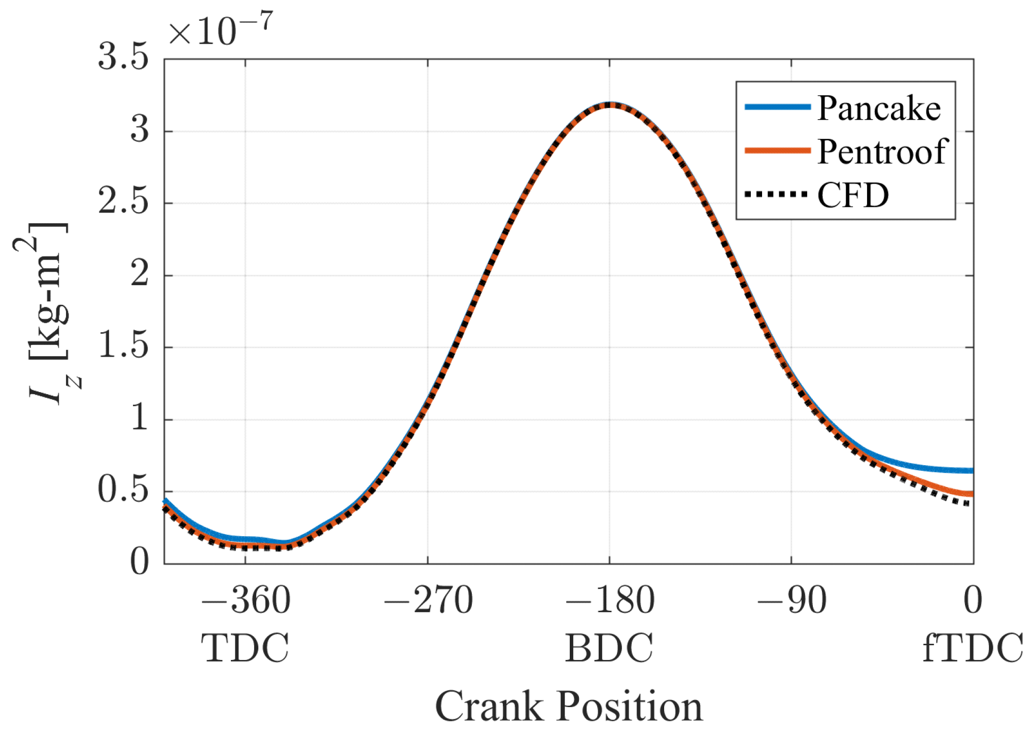
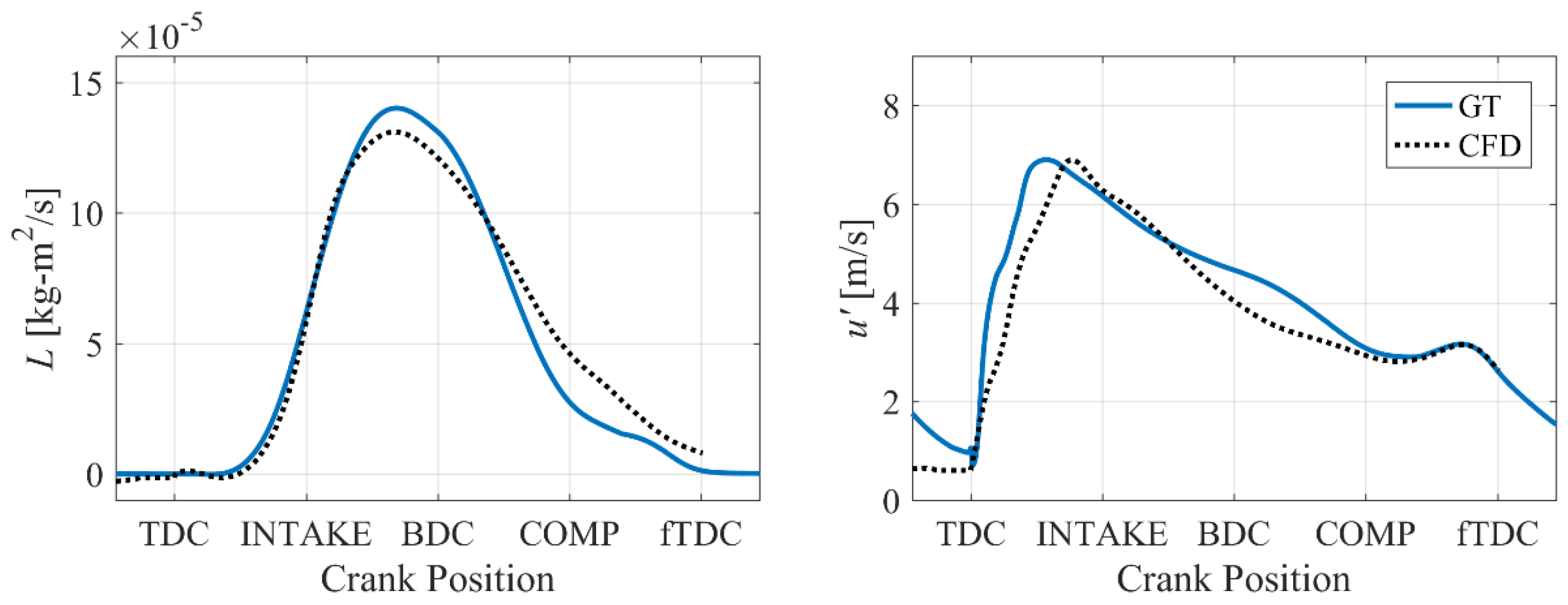
• describes the port characterization methodology in detail, which is verified via comparing the model prediction with the transient CFD results. This port characterization facilitates 0D model to predict the detailed flow characteristics with accuracy comparable to 3D CFD regardless of operating condition, which is quite noteworthy for a 0D model.
• suggests a physics-based approach to calculate tumble generation and decay rates for given engine geometry, utilizing the pre-obtained detailed flow characteristics. This QD tumble model is integrated into the k-ε model to complete the new predictive turbulence model.
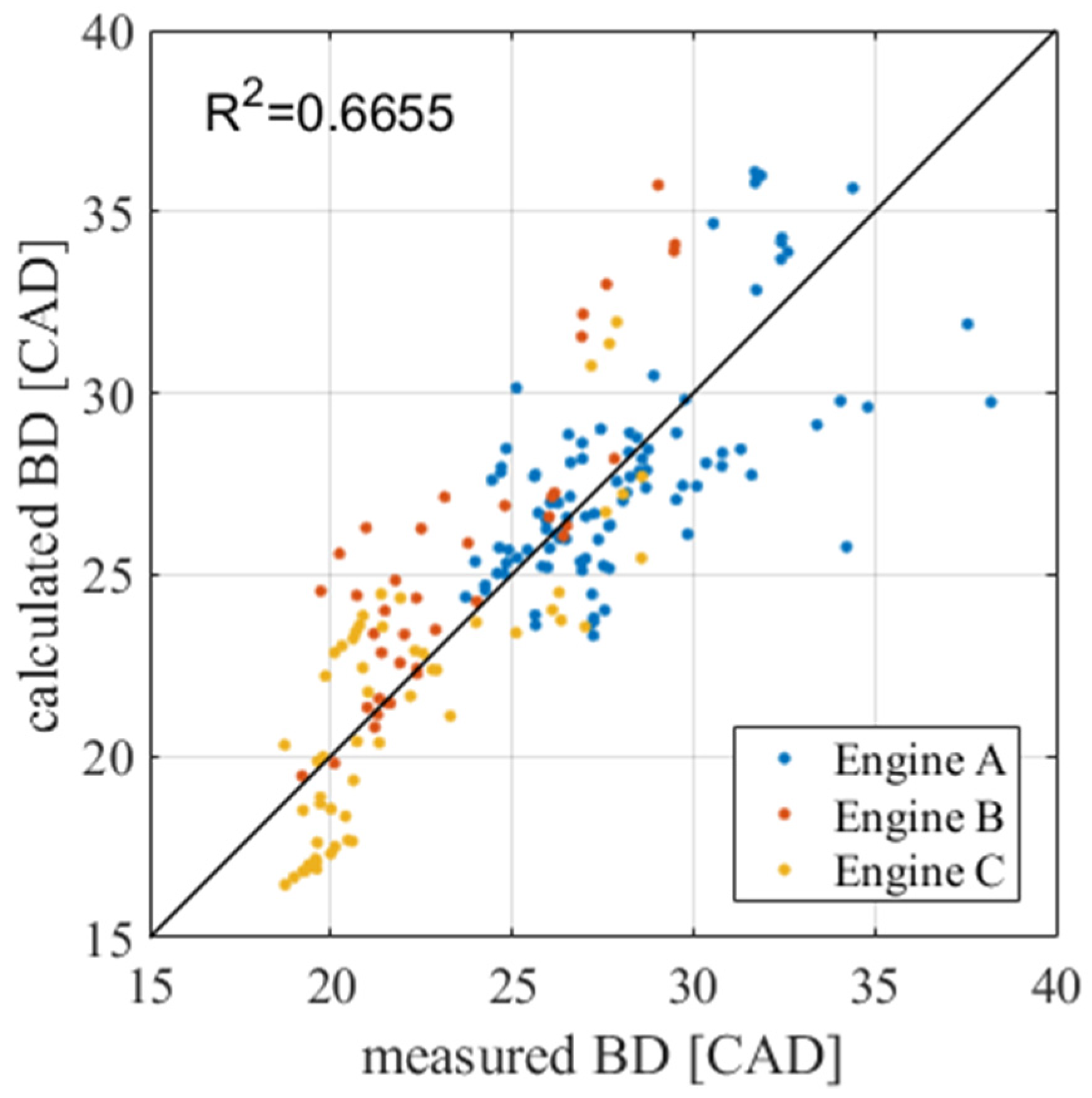
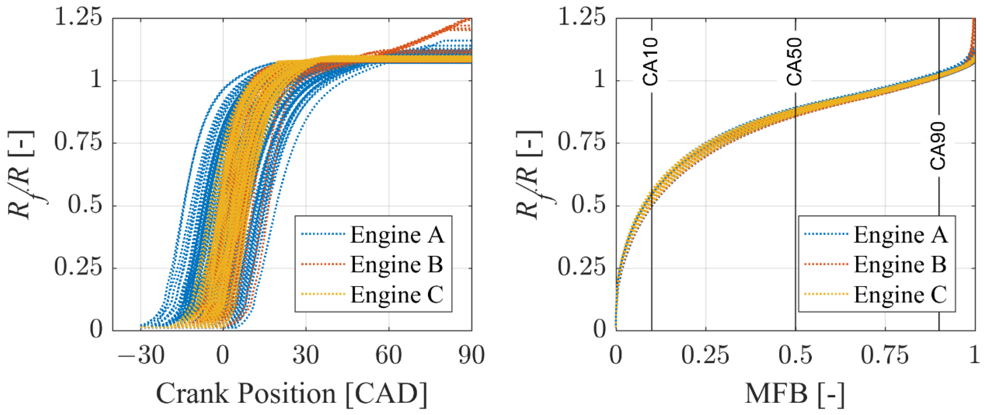
• demonstrates the validation of the developed model with engine experiment results to verify whether the model correctly considers for port and cylinder geometry and whether it is applicable for various operating conditions. An adequate correlation between the model and experiment results has been observed with fixed modeling constants, implying that the developed model could sufficiently capture the core physics related to engine geometry and operating condition.

The final validation results support the predictability of the new turbulence model, thus its potential as a part of a virtual engine. Moreover, it could be glimpsed that the model reliability can possibly be improved with the further advancement of other elements such as combustion model.

References

1. Ikeya, K.; Takazawa, M.; Yamada, T.; Park, S.; Tagishi, R. Thermal Efficiency Enhancement of a Gasoline Engine. SAE Int. J. Engines 2015, 8, 1579–1586. [Google Scholar] [CrossRef]
2. Hirooka, H.; Mori, S.; Shimizu, R. Effects of High Turbulence Flow on Knock Characteristics. SAE Trans. 2004, 113, 651–659. [Google Scholar]
3. Berntsson, A.W.; Josefsson, G.; Ekdahl, R.; Ogink, R.; Grandin, B. The Effect of Tumble Flow on Efficiency for a Direct Injected Turbocharged Downsized Gasoline Engine. SAE Int. J. Engines 2011, 4, 2298–2311. [Google Scholar] [CrossRef]
4. Ogink, R.; Babajimopoulos, A. Investigating the Limits of Charge Motion and Combustion Duration in a High-Tumble Spark-Ignited Direct-Injection Engine. SAE Int. J. Engines 2016, 9, 2129–2141. [Google Scholar] [CrossRef]
5. Achuth, M.; Mehta, P.S. Predictions of Tumble and Turbulence in Four-Valve Pentroof Spark Ignition Engines. Int. J. Engine Res. 2001, 2, 209–227. [Google Scholar] [CrossRef]
6. Bozza, F.; Teodosio, L.; De Bellis, V.; Fontanesi, S.; Iorio, A. Refinement of a 0D Turbulence Model to Predict Tumble and Turbulent Intensity in SI Engines. Part II: Model Concept, Validation and Discussion. SAE Technical Paper Series. 2018. [Google Scholar] [CrossRef]
7. Yoshihara, Y.; Nakata, K.; Takahashi, D.; Omura, T.; Ota, A. Development of High Tumble Intake-Port for High Thermal Efficiency Engines. SAE Technical Paper. 2016. [Google Scholar] [CrossRef]
8. Heywood, J.B. Internal Combustion Engine Fundamentals; McGraw-Hill Education: Columbus, OH, USA, 1988. [Google Scholar]
9. Li, Y.-f.; Liu, S.-l.; Shi, S.; Feng, M.; Sui, X. An investigation of in-cylinder tumbling motion in a four-valve spark ignition engine. J. Proc. Inst. Mech. Eng. Part D J. Automob. Eng. 2001, 215, 273–284. [Google Scholar] [CrossRef]
10. Falfari, S.; Forte, C.; Brusiani, F.; Bianchi, G.M.; Cazzoli, G.; Catellani, C. Development of a 0D Model Starting from Different RANS CFD Tumble Flow Fields in Order to Predict the Turbulence Evolution at Ignition Timing. SAE Technical Paper Series. 2014. [Google Scholar] [CrossRef]
11. Kent, J.; Mikulec, A.; Rimal, L.; Adamczyk, A.; Mueller, S.; Stein, R.; Warren, C. Observations on the effects of intake-generated swirl and tumble on combustion duration. SAE Trans. 1989, 98, 2042–2053. [Google Scholar]
12. Gosman, A.; Tsui, Y.; Vafidis, C. Flow in a Model Engine with a Shrouded Valve-A Combined Experimental and Computational Study. SAE Technical Paper. 1985. [Google Scholar] [CrossRef]
13. Dai, W.; Newman, C.E.; Davis, G.C. Predictions of in-cylinder tumble flow and combustion in SI engines with a quasi-dimensional model. SAE Trans. 1996, 105, 2014–2025. [Google Scholar]
14. Grasreiner, S.; Neumann, J.; Luttermann, C.; Wensing, M.; Hasse, C. A quasi-dimensional model of turbulence and global charge motion for spark ignition engines with fully variable valvetrains. Int. J. Engine Res. 2014, 15, 805–816. [Google Scholar] [CrossRef] [Green Version]
15. Fogla, N.; Bybee, M.; Mirzaeian, M.; Millo, F.; Wahiduzzaman, S. Development of a K-k-ε Phenomenological Model to Predict In-Cylinder Turbulence. SAE Int. J. Engines 2017, 10, 562–575. [Google Scholar] [CrossRef]
16. Kim, Y.; Kim, M.; Kim, J.; Song, H.H.; Park, Y.; Han, D. Predicting the Influences of Intake Port Geometry on the Tumble Generation and Turbulence Characteristics by Zero-Dimensional Spark Ignition Engine Model. SAE Technical Paper. 2018. [Google Scholar] [CrossRef]
17. Kent, J.; Haghgooie, M.; Mikulec, A.; Davis, G.; Tabaczynski, R. Effects of Intake Port Design and Valve Lift on In-Cylinder Flow and Burnrate. SAE Technical Paper. 1987. [Google Scholar] [CrossRef]
18. Baratta, M.; Misul, D.; Spessa, E.; Viglione, L.; Carpegna, G.; Perna, F. Experimental and numerical approaches for the quantification of tumble intensity in high-performance SI engines. Energy Convers. Manag. 2017, 138, 435–451. [Google Scholar] [CrossRef]
19. Kuwahara, K.; Watanabe, T.; Takemura, J.; Omori, S.; Kume, T.; Ando, H. Optimization of in-cylinder flow and mixing for a center-spark four-valve engine employing the concept of barrel-stratification. SAE Trans. 1994, 103, 1502–1513. [Google Scholar]
20. Benjamin, S. Prediction of barrel swirl and turbulence in reciprocating engines using a phenomenological model. In Proceedings of the Institute of Mechanical Engineers Conference on Experimental and Predictive Methods in Engine Research and Development, Birmingham, UK, 17 November 1993. [Google Scholar]
21. Ramajo, D.; Zanotti, A.; Nigro, N. Assessment of a zero-dimensional model of tumble in four-valve high performance engine. Int. J. Numer. Methods Heat Fluid Flow 2007, 17, 770–787. [Google Scholar] [CrossRef]
22. Kim, M.; Kim, Y.; Song, H.H. Development of Zero-Dimensional Spark Ignition Engine Model Considering Turbulence Formation in Various Intake Pressure Conditions and Intake Manifold Designs. In Proceedings of the 56th KOSCO Symposium, Jeonju, Korea, 10–12 May 2018. [Google Scholar]
23. Kim, N.; Ko, I.; Min, K. Development of a zero-dimensional turbulence model for a spark ignition engine. Int. J. Engine Res. 2018, 20, 441–451. [Google Scholar] [CrossRef]
24. Morel, T.; Mansour, N. Modeling of Turbulence in Internal Combustion Engines. SAE Technical Paper. 1982. [Google Scholar] [CrossRef]
25. Oh, S.; Cho, S.; Seol, E.; Song, C.; Shin, W.; Min, K.; Song, H.H.; Lee, B.; Jinwook, S.; Woo, S.H. An Experimental Study on the Effect of Stroke-to-Bore Ratio of Atkinson DISI Engines with Variable Valve Timing. J. SAE Int. J. Engines 2018, 11, 1183–1193. [Google Scholar] [CrossRef]
Figure 1. Classification of charge motions.
Energies 12 01898 g001
Figure 2. Distribution of mass flux on valve curtain area.
Energies 12 01898 g002
Figure 3. The sectional view of a pentroof cylinder showing the approaches of the tumble generation rate estimation: typical 0D tumble model (left) and the suggested QD tumble model (right).
Energies 12 01898 g003
Figure 4. Qualitative mass flow distribution across the valve curtain area at different valve lifts.
Energies 12 01898 g004
Figure 5. Fractional distribution of intake mass flow rate through each curtain area division.
Energies 12 01898 g005
Figure 6. Total (left) and divisional (right) mass flow rate over the gas exchange process (solid lines: GT-Power, dotted lines: transient CFD).
Energies 12 01898 g006
Figure 7. Divisional flow velocities passing valve curtain area (solid: QD, dotted: steady CFD).
Energies 12 01898 g007
Figure 8. Outline of actual (left) and simplified (right) pentroof geometry.
Energies 12 01898 g008
Figure 9. Comparison of the moment of inertia calculated by 0D and 3D model.
Energies 12 01898 g009
Figure 10. Modified velocity profile.
Energies 12 01898 g010
Figure 11. Flow chart of the new turbulence model.
Energies 12 01898 g011
Figure 12. Results of angular momentum and turbulent intensity under modeling constants sweep.
Energies 12 01898 g012
Figure 13. Comparison of angular momentum (left) and turbulent intensity (right) after calibration. CFD data is reproduced from [16], SAE International: 2018.
Energies 12 01898 g013
Figure 14. Comparison of near-TDC turbulent intensity under variations in intake pressure, engine speed, and intake port curvature ((solid lines: GT-Power, dotted lines: transient CFD).
Energies 12 01898 g014
Figure 15. Measured and calculated duration between ignition and 50% burn angle (BD0050).
Energies 12 01898 g015
Figure 16. Development of flame radius.
Energies 12 01898 g016
Figure 17. Correlation between simulation and experiment results (Engines A, B, and C).
Energies 12 01898 g017
Figure 18. Correlation between simulation and experiment results (Engines A, B, and C, high RMF cases excluded).
Energies 12 01898 g018
Figure 19. Model prediction with intake valve timing sweep (Engine A, 2000 rpm, 4.5 bar IMEP).
Energies 12 01898 g019
Figure 20. Averaged laminar flame speed and average turbulent intensity with intake valve timing sweep.
Energies 12 01898 g020
Figure 21. Correlation between simulation and experiment results (intake valve timing sweep).
Energies 12 01898 g021
Figure 22. Model prediction with intake valve timing sweep (2000 rpm, 4.5 bar IMEP).
Energies 12 01898 g022
Figure 23. Averaged laminar flame speed and average turbulent intensity with intake valve timing sweep.
Energies 12 01898 g023
Figure 24. Correlation between simulation and experiment results (intake valve timing sweep).
Energies 12 01898 g024