Day-Ahead Solar Irradiance Forecasting for Microgrids Using a Long Short-Term Memory Recurrent Neural Network: A Deep Learning Approach

Abstract

In microgrids, forecasting solar power output is crucial for optimizing operation and reducing the impact of uncertainty. To forecast solar power output, it is essential to forecast solar irradiance, which typically requires historical solar irradiance data. These data are often unavailable for residential and commercial microgrids that incorporate solar photovoltaic. In this study, we propose an hourly day-ahead solar irradiance forecasting model that does not depend on the historical solar irradiance data; it uses only widely available weather data, namely, dry-bulb temperature, dew-point temperature, and relative humidity. The model was developed using a deep, long short-term memory recurrent neural network (LSTM-RNN). We compare this approach with a feedforward neural network (FFNN), which is a method with a proven record of accomplishment in solar irradiance forecasting. To provide a comprehensive evaluation of this approach, we performed six experiments using measurement data from weather stations in Germany, U.S.A, Switzerland, and South Korea, which all have distinct climate types. Experiment results show that the proposed approach is more accurate than FFNN, and achieves the accuracy of up to 60.31 W/m² in terms of root-mean-square error (RMSE). Moreover, compared with the persistence model, the proposed model achieves average forecast skill of 50.90% and up to 68.89% in some datasets. In addition, to demonstrate the effect of using a particular forecasting model on the microgrid operation optimization, we simulate a one-year operation of a commercial building microgrid. Results show that the proposed approach is more accurate, and leads to a 2% rise in annual energy savings compared with FFNN.

1. Introduction

Around the world, countries are taking unprecedented steps to support renewable energy adoption. Currently, the number of photovoltaic (PV) installations is growing faster than any other renewable energy resource, driven mainly by sharp cost reductions and policy support [1]. In the United States, utility-scale photovoltaic capacity is projected to grow by 127 GW [2]. South Korea plans to increase its solar power generation fivefold by 2030 [3]. China, the world’s leading installer of PV, has a goal to reach 1300 GW of solar capacity by 2050 [4]. This increasing PV adoption is leading to increasing integration of PV into microgrids. To operate PV-based microgrids optimally, an accurate forecast of day-ahead solar power is necessary. However, solar PV power output is calculated from solar irradiance, resulting in a growing interest in solar irradiance forecasting. Some of the applications of solar irradiance forecasting in microgrids include economic dispatch, peak shaving, energy arbitrage, participation in the energy market, and uncertainty impact reduction.

Solar irradiance forecasting has been extensively studied in the literature. Generally, it can be broadly classified in terms of forecast horizons and model types. For the forecast horizon, forecasting can be categorized as very short-term [5], short-term [6], and medium-term [7,8]. Very short-term forecasting (a few minutes to 1 h) is used for real-time optimization, an important component of an energy management system. Short-term forecasting (3–4 h) is used for intraday market participation. Medium-term forecasting (typically a day ahead) is useful for day-ahead operation optimization and market participation.

Model types can be categorized as either data-driven or physical. Data-driven models use historical time series data. They can be further sub-categorized into statistical or machine learning models. Statistical models include autoregressive integrated moving average (ARIMA) [9], auto-regressive moving average (ARMA) [10], coupled autoregressive and dynamic system (CARD) [11], Lasso [12], and Markov models [13,14,15]. 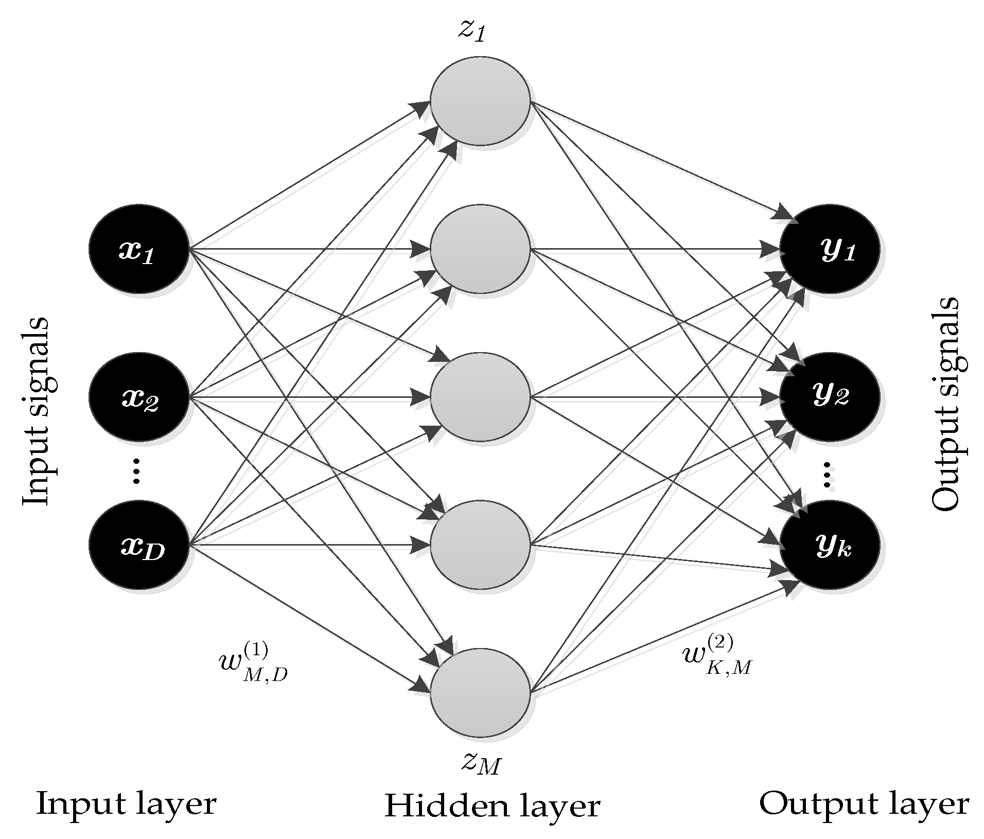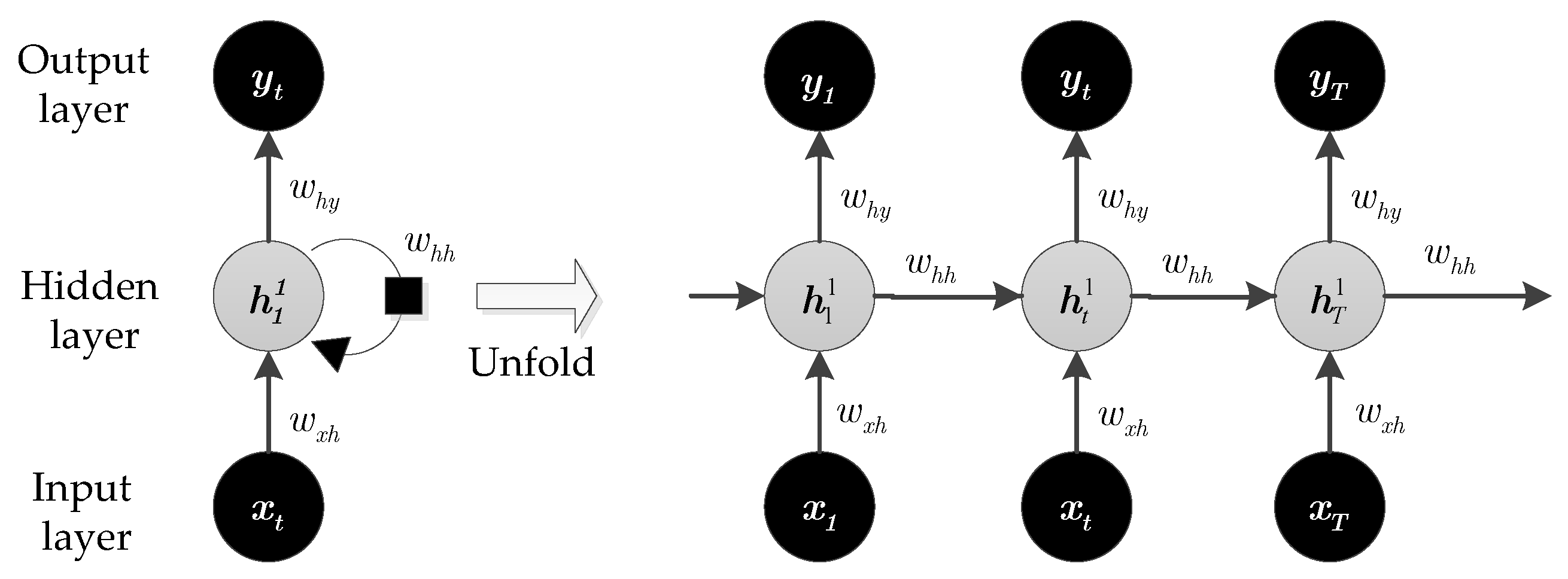Machine learning models [16] include support vector machine (SVM) [17,18], feedforward neural network (FFNN) [19], and recurrent neural network (RNN) [20]. Data-driven models can be further subdivided according to the type of input features they use to train the model. A forecasting model that uses only a target time-series (solar irradiance in this case) as an input feature is referred to as a nonlinear autoregressive (NAR) model. On the other hand, if a model uses additional exogenous inputs, such as temperature and humidity, it is referred to as a nonlinear autoregressive with exogenous inputs (NARX) model. Physical models use numerical weather prediction (NWP) [21,22,23], which shows good performance for forecast horizons from several hours up to six days.

Until recently, the forecasting domain has been largely influenced by statistical models. There is an increasing shift to machine learning models, due in part to the increasing availability of historical data. These models have come into serious contention with classical statistical models in the forecasting community [24]. Machine learning models use historical data to learn the stochastic dependency between the past and the future. A wealth of studies conclude that these models outperform statistical models in solar irradiance forecasting.

Table 1. Previous studies on a day-ahead solar irradiance forecasting.

Location	Dataset Size		Model	Publication	Reference
	Train Set	Test Set		Year
Japan	1827	365	FFNN	1999	[25]
Japan	333	4	RNN, RBFN	2007	[26]
China	7992	744	DRWNN	2008	[40]
Italy	Unknown	Unknown	FFNN	2010	[27]
France	6574	547	FFNN	2010	[28]
Spain	219,439	60,768	FFNN	2011	[29]
China	670	74	RBFN	2011	[38]
Spain	1241	219	FFNN	2011	[30]
USA	237	158	FFNN	2011	[31]
Turkey	1096	365	SVM	2014	[17]
Spain	292	73	ELM	2014	[36]
Macau	723	38	FFNN, SVM, KNN, MLR	2014	[32]
France	Unknown	Unknown	FFNN	2014	[34]
France	2920	730	FFNN	2014	[33]
New Zealand	Unknown	Unknown	RNN	2015	[39]
Italy	876	584	FFNN	2015	[46]
Italy	120	30	FFNN	2017	[35]
Seven countries	164,350	365	LSTM	2018	[20]
Four countries	16,973	2190	LSTM	2019	This study

tabulates the previous studies on day-ahead solar irradiance forecasting. We report the study location, dataset size (number of examples, which correspond to a day measurement), and the machine learning model used. The models include FFNN, RNN, and SVM, among others. FFNN is by far the most widely applied algorithm in the literature. Kemmoku et al. [25] used multi-stage FFNN to forecast a day-ahead solar irradiance in Omaezaki, Japan. The results showed that the mean error reduces from about 30% (by single-stage FFNN) to about 20% (by multi-stage FFNN). Yona et al. [26] proposed a method for forecasting day-ahead solar irradiance using RNN and a radial basis function neural network (RBFNN). They found that both RNN and RBFNN outperform FFNN. In [27], Mellit et al. used FFNN with two hidden layers to forecast solar irradiance for day-ahead in Trieste, Italy. The inputs to their model were mean daily solar irradiance, mean daily temperature, and time of day. Paoli et al. [28] used 19 years of data from Corsica Island, France, to fit an FFNN model to forecast a day-ahead solar irradiance. The study compared the performance of FFNN and Markov chains, Bayesian inference, k-nearest neighbor (KNN), and autoregressive (AR) models, and found that FFNN outperforms all these models. In [29], Linares et al. used FFNN to generate daily solar irradiance in locations without ground measurement. The model was developed using 10 years of data from 83 ground stations in Andalusia, Spain. In [30], they applied three models to predict day-ahead solar irradiance over Spain. The models are Bristow–Campbell, FFNN, and Kernel Ridge Regression. They concluded that FFNN produces the most accurate result. In [31], they used predicted meteorological variables from the US National Weather Service database to predict day-ahead solar irradiance using FFNN. Long et al. [32] used four different machine learning methods, including FFNN, to forecast day-ahead solar irradiance. They concluded that none of the models can outperform others in all scenarios. In [33], Voyant et al. applied FFNN to forecast day-ahead solar irradiance. They reported interesting analyses, such as the effects of using endogenous and exogenous data, and the performance of three different FFNN architectures. The findings indicated that using exogenous data improves the model accuracy and that multi-output FFNN has better accuracy than the two other architectures. Other authors that used FFNN and achieved satisfactory results include [34,35].

Other machine learning models besides FFNN have been seen in the literature. In [36], the authors forecasted day-ahead solar irradiance by applying Coral Reefs Optimization (CRO) and trained their neural network using an extreme learning machine (ELM) approach. The ELM was used to solve the forecasting problem, and then CRO was applied to evolve the weights of the neural network in order to improve the solution. In [37], the authors used a partial function linear regression model to forecast a daily solar power output. In this model, the intra-day time-varying pattern of output power was incorporated into the forecasting framework. In [38], Chen et al. used RBFNN to forecast solar power output by first training a self-organized map to classify the local weather type for 24-h ahead.

In [39], Ahmad et al. used an autoregressive RNN with exogenous inputs and weather variables to provide a day-ahead forecast of hourly solar irradiance in New Zealand. In [40], Cao and Lin combined RNN with a wavelet neural network, forming a diagonal recurrent wavelet neural network to perform day-ahead solar irradiance forecasting. They demonstrated improvement in accuracy using data from Shanghai and Macau. In [20], a comparative study of long short term memory (LSTM) in forecasting day-ahead solar irradiance was performed. The results suggest that LSTM outperforms many alternative models (including FFNN) by a substantial margin.

In this paper, we propose a deep LSTM-RNN using only exogenous inputs (i.e., without using solar irradiance as an input feature to the model) to forecast day-ahead solar irradiance. We note that we are not the first to use only exogenous inputs, as it was reported in [29], that exogenous inputs were used exclusively to train FFNN for day-ahead solar irradiance forecasting. However, we found that using this approach with LSTM is more accurate than with FFNN. Notably, the studies in Table 1 were trained and evaluated using data from a single country (with the exception of [20]); this makes their findings difficult to generalize because it does not take into account the changing spatial and climatic conditions across different locations. It is also important to point out that none of these studies experimented with a deep learning approach, even though that approach was found to be successful in electricity load forecasting [41], wind speed forecasting [42,43], and electricity price forecasting [44]. Finally, all the studies reviewed focused on forecasting accuracy without demonstrating the usefulness of the forecast. In this work, we used a microgrid design and analysis model developed in [45], to simulate a one-year optimal operation of a commercial building microgrid using the actual and forecasted solar irradiance.

In summary, the contributions of this work to the literature are threefold. First, we develop a model to predict solar irradiance using only exogenous inputs; this means the model can generate solar irradiance for a given location without past measurement of solar irradiance at the location. Second, we demonstrate that by using a deep learning approach, LSTM-RNN can achieve higher accuracy than other models; the model achieved higher accuracy in term of forecast skill than the results obtained from the previous studies cited. We demonstrate the performance of our approach using six datasets. Finally, we simulate a one-year operation of a microgrid, thereby demonstrating the usefulness of the forecasting model.

The rest of the paper is organized as follows: The theoretical background of deep learning, LSTM-RNNs, and FFNN are discussed in Section 2. In Section 3, we provide the details of the end-to-end problem formulation of an LSTM-RNN model for solving the solar irradiance forecasting problem. The results, analysis, and discussion are presented in Section 4. Section 5 provides the conclusion and describes future research work.

2. Deep Learning, FFNN, and LSTM; Theoretical Background

This section provides a theoretical background of the models used in this work. We start with an overview of deep learning. We then introduce FFNN and LSTM-RNN.

2.1. Deep Learning

Deep learning is part of a broader family of machine learning techniques that use multiple processing layers to learn a representation of data with multiple levels of abstraction [47]. It discovers intricate structures in large datasets by using the backpropagation algorithm to indicate how a machine should change its internal parameters that are used to compute the representation in each layer from the representation in the previous layer [48]. Deep learning architectures include FFNN, RNN, deep belief networks (DBN), and restricted Boltzmann machine (RBM). Among these architectures, the most widely used are FFNN and RNN. Deep convolution neural networks (CNN), which are a family of FFNN, are remarkably good at processing images, video, and audio. Deep LSTMs, which are a family of RNN, are good with sequential data, such as text, speech, and time series. Deep learning is making major advances in many domains. It has outperformed other machine learning techniques in image recognition [49,50], speech recognition [51,52], natural language understanding [53], language translation [54,55], particle accelerator data analysis [56], potential drug molecule activity prediction [57], and brain circuit reconstruction [58]. However, its application in the solar irradiance forecasting is limited [59].

2.2. Feedforward Neural Network (FFNN)

An FFNN defines a mapping $y=f(x,W)$ and learns the value of the parameters W that result in the best function approximation. These networks are called FFNN because information flows through the function being evaluated from x, through the intermediate computations used to define f, and finally to the output y [60]. An FFNN consists of an input layer, an output layer, and one or more hidden layers between the input and output layer. As shown in Figure 1, the first hidden layer is connected to the input layer; its output is then passed to the next hidden layer or output layer. The output layer makes a prediction or classification decision using the value computed in the hidden layers. For the FFNN in Figure 1, we can construct M linear combinations of the input variables x₁, …, x_D in the form:

$$a_j={\displaystyle \sum _{i=1}^D{w}_{ji}^{(1)}\cdot x_i+b_j^{(1)}}$$

(1)

where $j=1,\dots ,M$. The superscript (1) in Equation (1) indicates that corresponding parameters are in the first layer of the network; $w_{ji}^{(1)}$ and $b_j^{(1)}$ are the weights and biases; $j$ and M are the index and total number of linear combination of the input variables, respectively; $i$ and D are the index and total number of the input variables, respectively; $a_j$ is the activation, which can be transformed using a differentiable, nonlinear activation function. The nonlinear activation functions can be logistic sigmoid, tanh, rectified linear unit (ReLu), etc. as in

$$a_j={\displaystyle \sum _{i=1}^D{w}_{ji}^{(1)}\cdot x_i+b_j^{(1)}}$$

(2)

The quantity z_j is called hidden unit and $\sigma$ is the logistic sigmoid. Following (1), these values are again linearly combined to give output unit activations:

$$a_k={\displaystyle \sum _{j=1}^M{w}_{kj}^{(2)}\cdot z_j+b_k^{(2)}}$$

(3)

where $k=1,\dots ,K,$ and K is the total number of outputs, $w_{kj}^{(2)}$ and $b_k^{(2)}$ are the weights and biases. This transformation corresponds to the second layer of the network. Finally, the output unit activations are transformed using an appropriate activation function to give a set of network outputs y_k.

$$y_k(\mathrm{X},\mathrm{W})=\sigma \left({\displaystyle \sum _{j=1}^M{w}_{kj}^{(2)}h\left({\displaystyle \sum _{i=1}^D{w}_{ji}^{(1)}\cdot x_i+b_j^{(1)}}\right)}+b_k^{(2)}\right)$$

(4)

In summary, the FFNN model is a nonlinear function from a set of input variables {x_i}s to set of output variables {y_k} controlled by a vector W of adjustable parameters [61].

FFNN learns by computing the error of the output of the neural network for a given sample, propagating the error back through the network while updating the weight vectors in an attempt to reduce the error. FFNNs are very powerful and are applied to many challenging problems in many fields.

2.3. Long Short Term Memory Recurrent Neural Network (LSTM-RNN)

RNNs are members of a class of artificial neural network (ANN) where a connection between nodes forms a directed graph along a sequence, enabling the network to exhibit temporal dynamic behavior for a time sequence. Given an input sequence x = (x₁, …, x_T), standard RNNs compute the hidden vector sequence h = (h₁, …, h_T) and output vector sequence y = (y₁, …, y_T) by iterating Equations (5) and (6) from t = 1 to T:

$$h_t=\mathcal{H}(W_{\mathit{xh}}\cdot x_t+W_{\mathit{hh}}\cdot h_{t-1}+b_h)$$

(5)

$$y_t=W_{\mathit{hy}}\cdot h_t+b_y$$

(6)

where W_xh, W_hh, W_hy terms respectively denote input-hidden, hidden-hidden, and hidden-output weight matrices. The b_h and b_y terms denote hidden and output bias vectors, respectively. The term $\mathcal{H}$ is the hidden layer activation function. It is usually an elementwise application of the sigmoid function. Figure 2 shows an RNN network and the unfolding in time of its forward computation. The artificial neurons get inputs from other neurons at previous time steps.

RNNs, in contrast to FFNNs, have a feedback connection. Their output depends on the current input to the network, and the previous inputs, outputs, and/or hidden states of the network. RNNs are very powerful dynamic systems, but training them has proved to be difficult because the back propagated gradients either grow or shrink at each time step, so they typically explode or vanish over several time steps [62]. To solve this problem, one idea is to provide an explicit memory to the network. The first proposal of this kind is LSTM.

LSTM units are building units for layers of RNNs. They were proposed in 1997 by Hochreiter and Schmidhuber [63] and improved by Gers et al. [64]. They were developed to solve the problem of vanishing gradient that occurs while training conventional RNNs. A typical LSTM unit is composed of an input gate, forget gate, output gate, and a cell unit. Figure 3 illustrates a single LSTM unit. It is a version of the LSTM discussed in [64]. The cell serves as a memory and remembers values over an arbitrary time interval. The input gate, forget gate, and output gate controls the flow of information into and out of the cell. The basic operations of the LSTM can be described as follows: (1) When the input gate is activated, new input information accumulates in the memory cell. (2) When the forget gate is activated, the cell forgets past status. (3) When the output gate is activated, the latest cell output propagates to the ultimate state.

The forward propagation equations of LSTM are given in Equations (7)–(11). The most important component is the cell unit c_t It has a linear self-loop that is controlled by a forget gate unit f_t, which sets the forward contribution of c_t−1 to a value between 0 and 1:

$$f_t=\sigma (W_{xf}\cdot x_t+W_{hf}\cdot h_{t-1}+b_f)$$

(7)

The LSTM cell internal state is thus updated as follows, but with a conditional self-loop weight f_t:

$$c_t=f_t\cdot c_{t-1}+i_t\cdot \tanh (W_{xc}\cdot x_t+W_{hc}\cdot h_{t-1}+b_c)$$

(8)

The external input unit i_t is calculated similarly to the forget gate, but with its own parameters:

$$i_t=\sigma (W_{xi}\cdot x_t+W_{hi}\cdot h_{t-1}+b_i)$$

(9)

The output h_t of the LSTM cell can also be shut off, via the output gate o_t, which also uses a sigmoid unit for gating:

$$h_t=o_t\cdot \tanh (c_t)$$

(10)

$$o_t=\sigma (W_{xo}\cdot x_t+W_{ho}\cdot h_{t-1}+b_o)$$

(11)

where i, f, o, and c are the input gate, forget gate, output gate, and cell, all of which are the same size as the hidden vector h, and W is the weight matrix. The bias terms (b_i, b_f, b_c, and b_o) are omitted for clarity. An RNN composed of LSTM units is called an LSTM network. LSTM networks have proven to be more effective than conventional RNNs, especially when they have several layers for each time step [65].

3. Problem Formulation

In this section, we develop the model for forecasting the 24-h global horizontal irradiance (GHI). Since GHI is the irradiance falling on a horizontal surface, and PV arrays are usually installed inclined to the horizontal plane, we need to account for this inclination when calculating solar irradiance incident on the PV array. Many models of varying complexity have been developed for calculating incident solar irradiance. Among these models, the HDKR model [66] is the most widely used. Its results are calculated as shown in Equation (12) below:

$$G_{inc}=(G_b+G_d\cdot A_i)\cdot R_b+G_d(1-A_i)\cdot \left(\frac{1+\cos \beta }{2}\right)\cdot \left(1+f\cdot {\sin }^3\left(\frac{\beta }{2}\right)\right)+G\cdot {\rho }_g\left(\frac{1-\cos \beta }{2}\right)$$

(12)

where G is the GHI, G_b is the beam radiation, G_d is the diffuse radiation, $\beta$ is the slope of the surface in degrees, ${\rho }_g$ is the ground reflectance, R_b is the ratio of the beam radiation on the tilted surface to beam radiation on the horizontal surface, A_i is the anisotropy index which is a function of the transmittance of the atmosphere for beam radiation, and f is the factor used to account for cloudiness. The power produced by the PV modules can be calculated from the incident irradiance calculated in Equation (12) as follows [67,68]:

$$P_{pv}=P_{pv,STC}\cdot \frac{G_{inc}}{G_{inc,STC}}[1+k_T\cdot (T_{cell}-T_{cell,STC})]$$

(13)

where P_pv,STC is the rated PV power at standard test conditions (kW), k_T is the temperature coefficient of power (%/°C), T_cell is the PV cell temperature (°C), T_cell,STC is the PV cell temperature at standard test conditions (25 °C), G_inc,STC is the incident solar irradiance at standard test conditions (1 kW/m²), and G_inc is the incident solar irradiance on the plane of the PV array (kW/m²). The cell temperature, T_cell, is calculated in Equation (14):

$$T_{cell}=T_{amb}+\frac{G_{inc}}{800}\cdot [NOCT-20]$$

(14)

where T_amb is the ambient temperature and NOCT is an acronym for the nominal operating cell temperature, a constant that is defined under the ambient temperature of 20 °C, incident solar irradiance of 800 W/m², and wind speed of 1 m/s.

3.1. Framing the Problem

Solving a forecasting problem by using historical data has a strong theoretical background. Two approaches to this type of problem come from statistical forecasting theory and dynamic system theory. Statistical forecasting theory assumes that an observed sequence is a specific realization of a random process, where the randomness arises from many independent degrees of freedom interacting linearly [69]. In dynamic system theory, the view is that apparently random behavior may be generated by deterministic systems interacting nonlinearly with only a small number of degrees of freedom [70]. The problem of time series forecasting can be framed as a supervised learning problem, which follows from dynamic system theory. Supervised learning is a machine learning algorithm that learns an input to output mapping function from example input-output pairs [71].

3.1.1. Problem Definition

Given historical weather data together with categorical features such as the hour of day and month of the year, we can forecast a day-ahead solar irradiance. To define the problem formally, we let $i\in {\mathbb{N}}_M$ represents an example in the dataset where M is the total number of examples in the dataset, $t\in {\mathbb{N}}_T$ represents the time step, where T represents the prediction horizon (24 h for day-ahead forecasting), W represents the length of the lookback window, and d denotes feature dimension. Given a dataset $\mathit{S}=\{{\mathit{x}}^{(i)};{\mathit{y}}^{(i)}{\}}_{i=1}^M$, where ${\mathit{x}}^{(i)}\subseteq {\mathbb{R}}^{d\times (t-W:t-1)}$ is an input matrix, $\{t-W:t-1\}$ is a temporal window, ${\mathit{y}}^{(i)}\subseteq {\mathbb{R}}^d$ is a multidimensional output vector over the space of real-valued outputs; determine $p\left(\mathit{y}\right|\mathit{x};\Theta )$, where $\mathit{y}\subseteq m\times {\mathbb{R}}^d$ and $\mathit{x}\subseteq m\times {\mathbb{R}}^{d\times (t-W:t-1)}$ are the concatenation of all outputs and inputs, respectively, and $\Theta$ represents model parameters, such that:

$$\mathrm{Distance}(p_{\mathrm{model}}(\mathit{y}|\mathit{x};\Theta )\left|\right|p_{\mathrm{empirical}}(\mathit{y}|\mathit{x}))$$

(15)

is minimized.

3.1.2. Performance Metrics

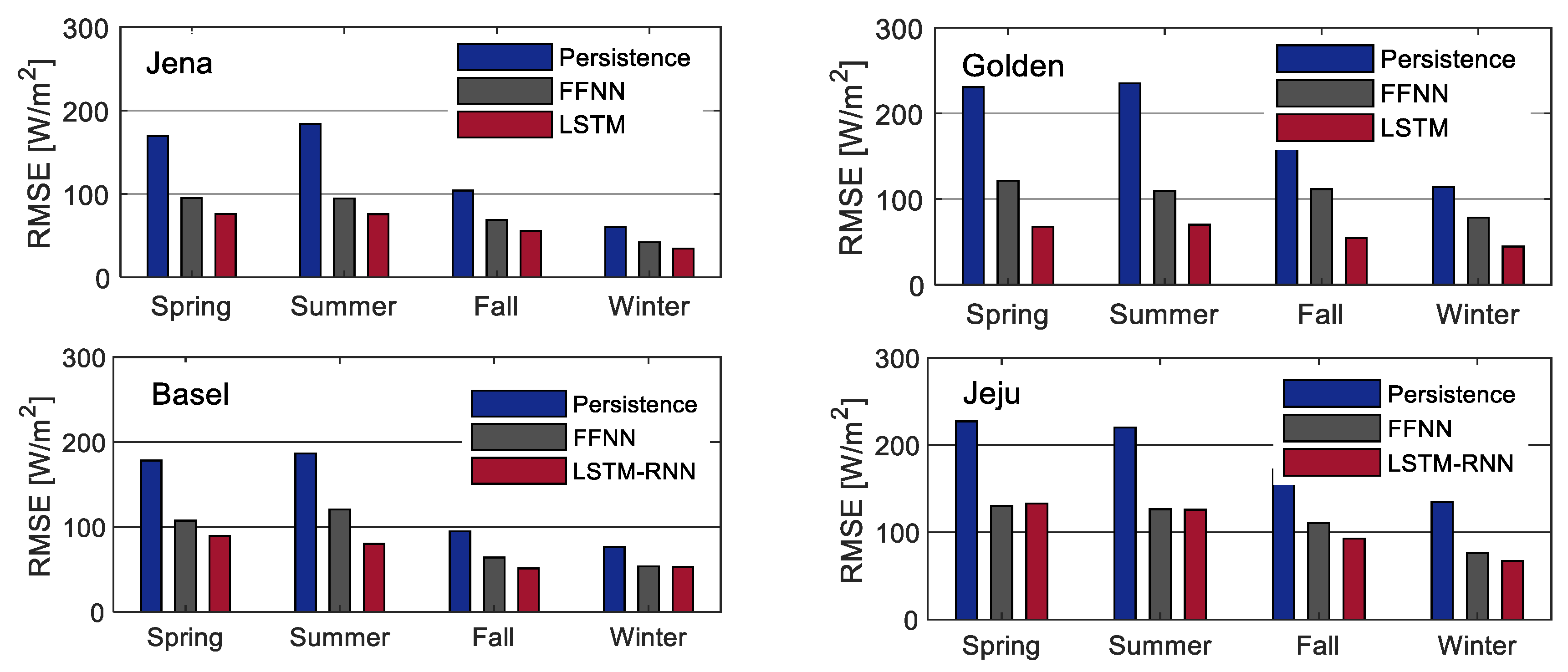
In order to evaluate the model’s performance, we need to choose a metric to measure the prediction accuracy. There are many issues that arise when choosing a metric as noted in [72,73]. Those authors observed that many metrics are not generally applicable, can be infinite or undefined in some cases, and can produce misleading results. Nevertheless, root mean square error (RMSE) and mean absolute error (MAE) are widely used in the literature. The equations for calculating RMSE and MAE are given respectively in Equations (16) and (17).

$$RMSE=\sqrt{\frac{1}{T\cdot M}{\displaystyle \sum _{i=1}^M{\displaystyle \sum _{t=1}^T{(h(x_t^{(i)})-y_t^{(i)})}^2}}}$$

(16)

$$MAE=\frac{1}{T\cdot M}{\displaystyle \sum _{i=1}^M{\displaystyle \sum _{t=1}^T\left|(h(x_t^{(i)})-y_t^{(i)})\right|}}$$

(17)

where M is the number of examples in the dataset, x⁽ⁱ⁾ is a vector of feature values of the ith example in the dataset, y⁽ⁱ⁾ is the desired output value of the ith example, h is the system prediction function. Note that using only RMSE and MAE as a measure of forecast accuracy can be misleading because they do not convey a measure of variability in the time series data. A metric that tries to address this issue is the forecast skill, proposed in [74]. Forecast skill gives the relative measure of improvement in prediction over the persistence model, which is also known as the naive model. It is given by Equation (18).

$$s=\left(1-\frac{U}{V}\right)\cdot 100$$

(18)

A typical forecast model should have a value of s between 0–100, with a value of 100 indicating perfect forecast, and a value of 0 indicating the model has an equal skill to persistence model. U and V are calculated over the same dataset, where $U\in \{MAPE,RMSE\}$ and $V\in \{MAP{E}_{persistence},RMS{E}_{persistence}\}$. Even though we used RMSE to evaluate the models in this paper, our motivation for also computing the MAE metric is for comparison with previous works, and to allow comparison with future works. For a comprehensive treatment of various performance metrics used in solar irradiance forecasting, interested readers can refer to [72,73].

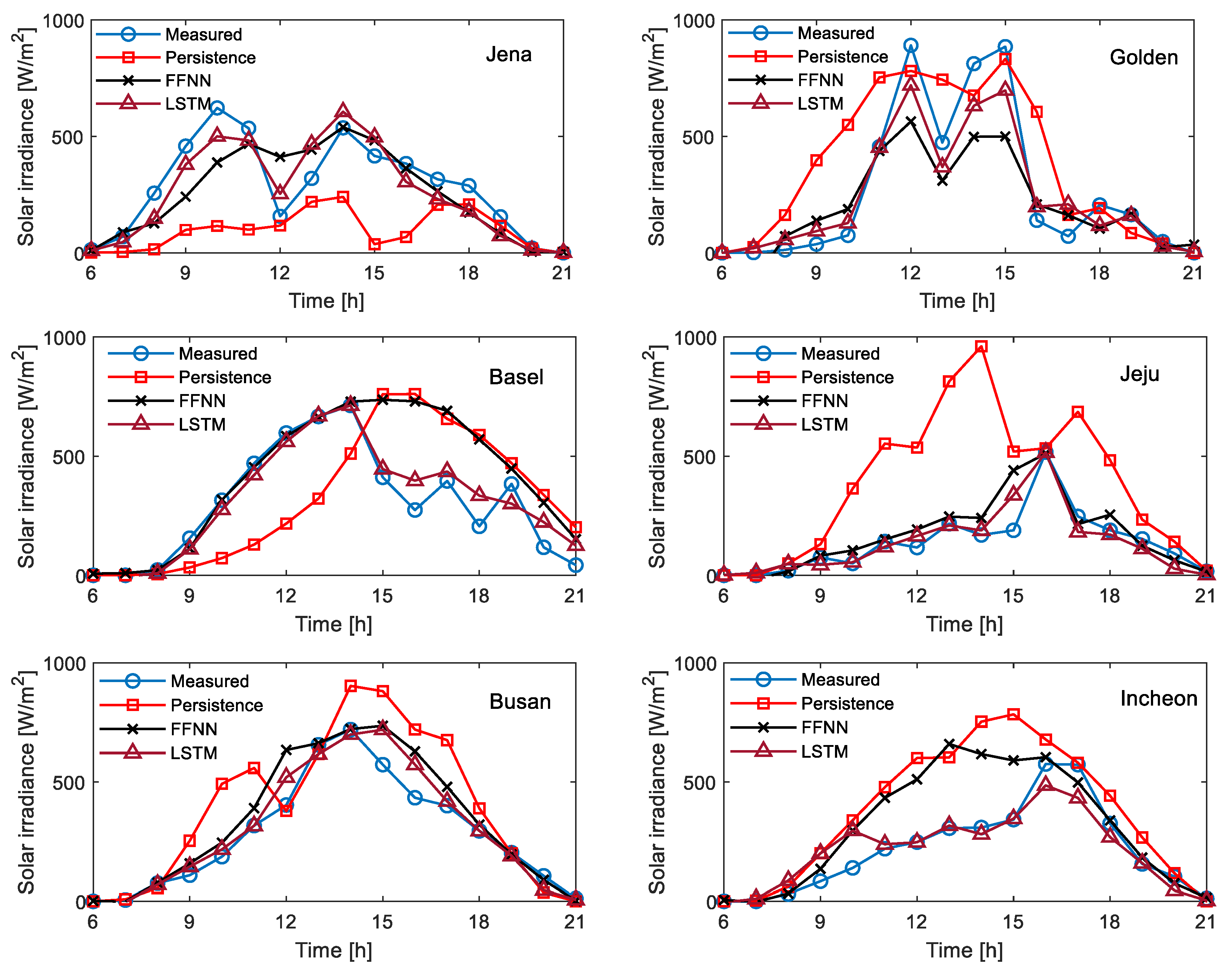
We use a day-ahead persistence model as a reference, which is a standard approach in the irradiance forecasting literature. This model assumes that the current conditions will repeat for the specified time horizon. In particular, the persistence model sets the irradiance value of the previous day to be the day-ahead predicted values.

3.2. Data Engineering

3.2.1. Data Description

A comprehensive evaluation of solar irradiance forecasting method should include multi-location based experiments, as this will increase confidence in the results. With this in mind, in this work, six datasets from four different countries were used. The countries selected have diverse climatic conditions and topographical features. These datasets are from Saaleaue Weather Station at the Max Planck Institute of Biochemistry in Jena, Germany [75]; Solar Radiation Research Laboratory (SRRL) in Golden, Colorado, USA [76]; Weather Station in Basel, Switzerland [77]; Korea Meteorological Administration (KMA) Weather Stations in Jeju, Busan, and Incheon [78].

Table 2. Datasets locations and climate types.

Location	Latitude (°)	Longitude (°)	Elevation (m)	Climate Type (Koppen Classification)	Size (Years)
Jena, Germany	50.9288	11.5899	149	Oceanic	7
Golden, U.S.A.	39.7329	−105.2389	1733	Semiarid	12
Basel, Switzerland	47.5584	7.5733	279	Temperate Atlantic	12
Jeju, South Korea	33.4890	126.4983	19	Humid subtropical	9
Busan, South Korea	35.1796	127.7669	20	Humid subtropical	9
Incheon, South Korea	37.4563	126.7052	45	Humid subtropical	9

summarizes information about latitude, longitude, elevation above sea level, climate type according to the Koppen classification system, and the sizes of the datasets for all the six locations.

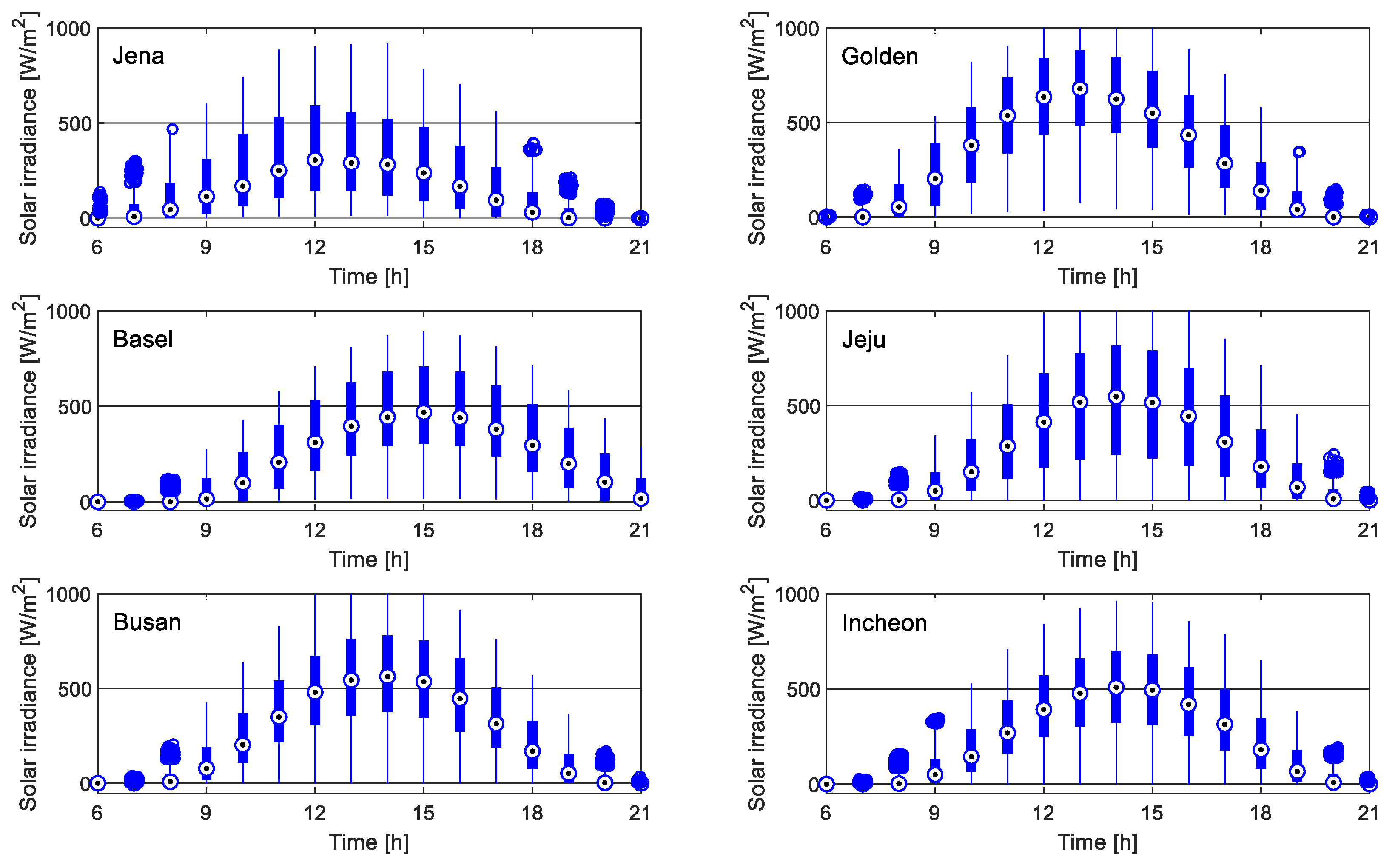
The weather variables collected in each location and their Pearson correlation coefficient (PCC) with solar irradiance is shown in

Table 3. Meteorological parameters and their Pearson Correlation Coefficient (PCC) with solar irradiance.

Variable	PCC
	Jena	Golden	Basel	Jeju	Busan	Incheon
Solar irradiance	1	1	1	1	1	1
Dry bulb temperature	0.5411	0.4084	0.4857	0.3087	0.2938	0.2595
Dew point temperature	0.2483	0.1188	0.1211	0.1305	0.0671	0.0634
Relative humidity	−0.6671	−0.3176	−0.5788	−0.3030	−0.2915	−0.3801
Wind speed	x	0.0342	0.0632	0.1651	0.1842	0.1463
Wind direction	x	x	0.0354	−0.0036	0.0376	0.1871
Precipitation	x	−0.016	−0.1000	−0.0662	−0.0687	−0.0625
Total cloud cover	x	0.2255	−0.2569	0.0991	−0.0229	−0.0251

. PCC is a measure of the correlation between two variables. It has a value between +1 and −1, where 1 is total positive linear correlation and −1 is total negative linear correlation. Given two variables (X, G), the formula for computing PCC is given below:

$$\mathrm{PCC}(X,G)=\frac{1}{N-1}{\displaystyle \sum _{i=1}^N\left(\frac{\overline{X_i-{\mu }_X}}{{\sigma }_X}\right)}\left(\frac{G_i-{\mu }_G}{{\sigma }_G}\right)$$

(19)

where $\mu$ and $\sigma$ are the mean and standard deviation of the variables (X, G), and N is the number of observations in each variable. The boxplots of solar irradiance for the six datasets are shown in Figure 4.

3.2.2. Data Division

We divided the data into three subsets: A training set, a validation set, and a test set. We used the training set to train the models and the validation set for hyperparameter optimization, feature selection, and regularization. The test set, which is the out-of-sample data, was used for final evaluation to select the best model.

Table 4. Training, validation and test sets.

Datasets	Periods	Number of Examples
Jena
Training set	1 January 2003–31 December 2008	2190
Validation set	1 January 2009–31 December 2009	365
Test set	1 January 2010–31 December 2010	365
Golden
Training set	1 January 2006–31 December 2015	3650
Validation set	1 January 2016–31 December 2016	366
Test set	1 January 2017–31 December 2017	365
Basel
Training set	1 January 2007–31 December 2016	3651
Validation set	1 January 2017–31 December 2017	365
Test set	1 January 2018–31 December 2018	365
South Korea
Training set	1 January 2009–31 December 2015	2554
Validation set	1 January 2016–31 December 2016	366
Test set	1 January 2017–31 December 2017	365

shows the data division and the number of examples in each subset. Note that in South Korea there are three datasets from Jeju, Busan, and Incheon, which are all divided in the same way.

3.2.3. Feature Selection

One of the central problems of time series supervised learning is identifying and selecting the relevant features for accurate forecasting. Feature selection improves the performance of a prediction by eliminating irrelevant features, reducing the dimension of the data, and increasing training efficiency. For solar irradiance forecasting, previous studies have discussed feature selection extensively [79,80,81,82]. In this study, the goal is to select the subset of features that are both easily obtainable for any location and that correlate with the solar irradiance. We did not rank the importance of features based on their PCC values because a feature can be irrelevant by itself but can provide a significant performance improvement when taken with other features [83]. There are two widely used approaches to the feature selection problem [84]: The wrapper and the filter approach. The wrapper approach consists of using an evaluation metric (in this paper, RMSE) of the machine learning algorithm to assess the space of all possible variable subsets. In the filter approach, heuristic measures are used to compute the relevance of a feature in a preprocessing stage without actually using the machine learning algorithm. In this paper, we used the former approach [85] since we have a small number of features to select from. We found that the subset of dry-bulb temperature, dew point temperature, and relative humidity comprise the most relevant set of features. This implies that to forecast day-ahead solar irradiance, we do not need previous days solar irradiance as an input feature to our forecasting model. Finally, we added two categorical features, the hour of the day (1–24) and the month of the year (1–12), which improved the prediction accuracy of the models.

3.2.4. Data Preparation

Before applying data to a machine learning algorithm, it is necessary to clean the data to fix or remove outliers and fill in any missing values. There are no missing values in the Golden and Basel datasets. In the Jena, Jeju, Busan, and Incheon datasets, there are a few missing values representing less than 1% of the entire dataset. We replaced the missing values using linear regression fit. We note that more sophisticated techniques such as Kalman filters could be used to replace the missing values [86]; however, considering there are just a few values to replace, this simple method will suffice.

Other data preparation steps in machine learning are feature scaling and encoding. Machine learning algorithms often perform poorly when the input numerical features have very different scales, so we rescaled the data to have a zero mean and unit variance. We encoded categorical features (the hour of the day and the month of the year) with 1-hot encoding. The one-hot encoder maps the original element from the categorical feature vector with M cardinality into a new vector with M elements, where only the corresponding new element is one while the rest of new elements are zeros.

3.3. Implementation Details: Training the LSTM Model

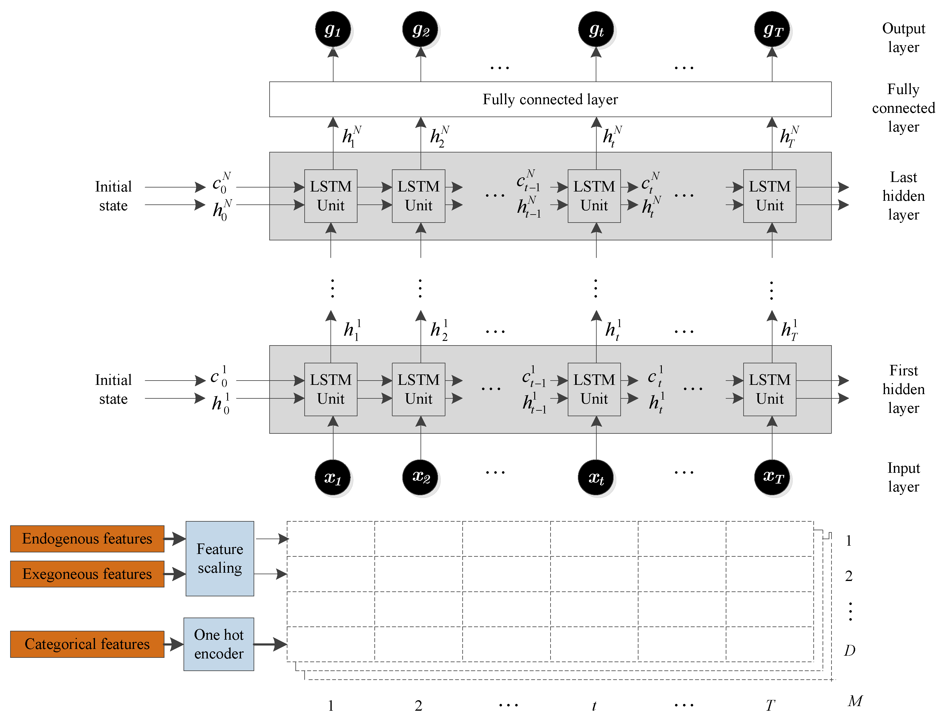
We used the Matlab Deep Learning Toolbox [87] to develop a forecasting framework used in this paper. The framework, shown in Figure 5, consists of an input layer, LSTM hidden layers, a fully connected layer, and an output layer. The input layer inputs the time series data into the network. The hidden layers learn long-term dependencies between time steps in the time series data. To make a prediction, the network ends with a fully connected layer and an output layer.

Each dashed-box in Figure 5 represents a training example that will be fed to the LSTM network. Note that $d\in D$ is the number of features (number of rows in the dashed-boxes), $t\in T$ is the number of time steps in the prediction horizon (number of columns in the dashed-boxes), and $m\in M$ is the number of training examples (total number of dashed-boxes). In summary, the input to the LSTM has three dimensions: D, T, and M.

For our proposed model, there are three exogenous features (dry bulb temperature, dew point temperature, and relative humidity), and two additional categorical features (the hour of the day and the month of the year), bringing the total number of features, D, to five. For the NARX model, there are two additional endogenous features (the solar irradiance for the previous two days), bringing the number of features, D, to seven. The number of columns, T, is the length of the prediction horizon, which is 24 for day-ahead forecasting. Finally, the third dimension, M, is the total number of the training examples in the dataset. The total dimension of the entire training set is $(D\times T\times M)$.

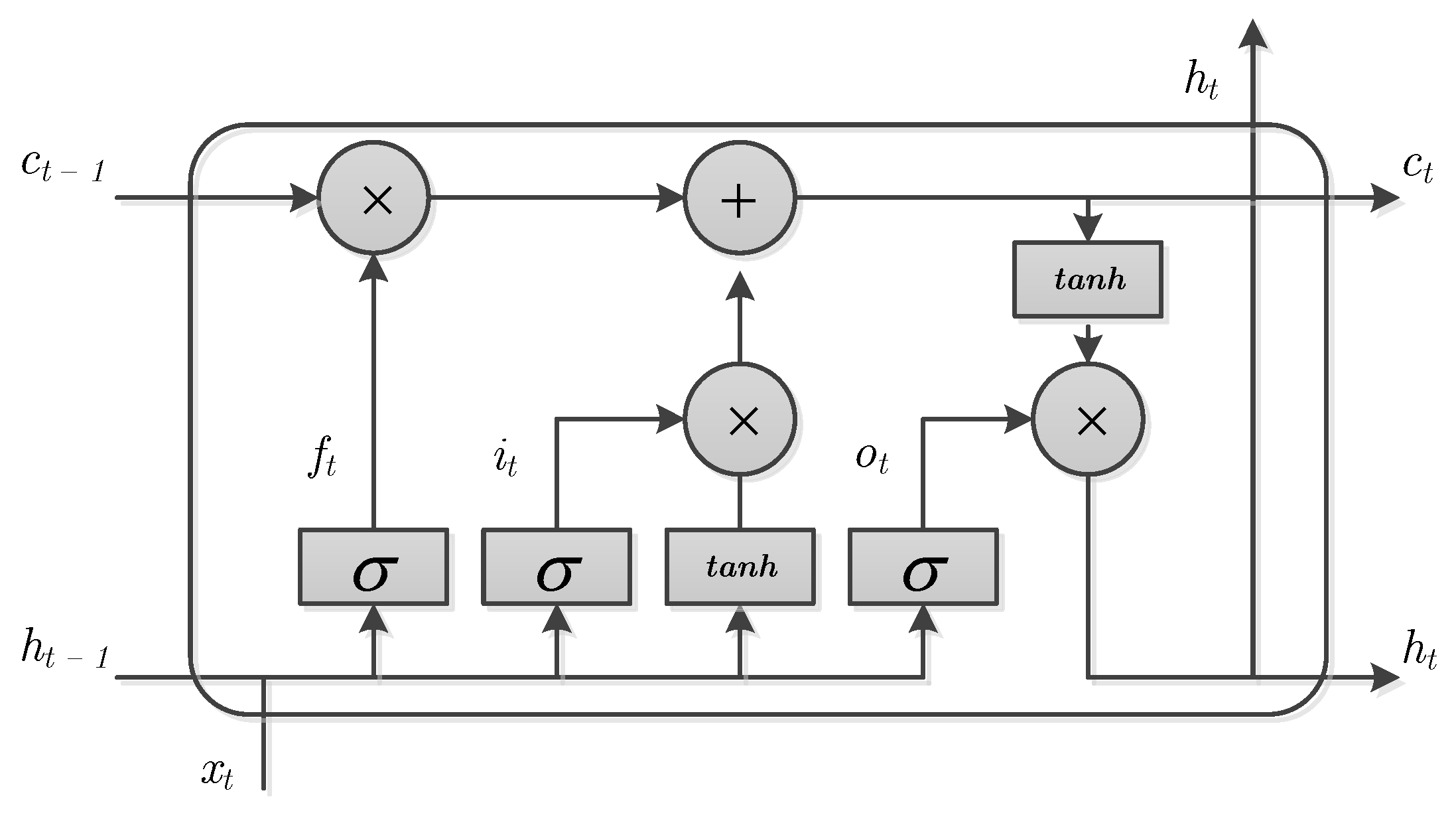
The first LSTM unit takes the initial state of the network and the first time step of the training example x₁, and computes the first output h₁ and the updated cell state c₁. At time step t, the unit takes the current state of the network (c_t−1, h_t−1) and the next time step of the training example x_t, and computes the output h_t and the updated cell state c_t. The final outputs are the day-ahead solar irradiance predictions, g₁, … g_T.

3.4. Hyperparameter Optimization

Achieving good performance with LSTM networks requires the optimization of many hyperparameters. These parameters affect the performance and time/memory cost of running the algorithm. The selection of hyperparameters often makes the difference between a mediocre and state-of-the-art performance for machine learning algorithms [88]. Even though there are some rules of thumb in the research community about the suitable values of these hyperparameters [89], optimization is necessary because the optimal values will depend on the type of data used in the comparisons, the particular data sets used, the performance criteria and various other factors. The hyperparameters that we optimized are tabulated in

Table 5. Hyperparameter optimization for LSTM model.

Hyperparameter	Value	Search Range
Learning rate	0.005	0.1, 0.01, 0.005, 0.001, 0.0005
Optimization solver	Adam	adam, sgdm, rmsprop
Feature scaling	Standard	Min-Max and Standard scaler
Number of layers	3	1, 3, 5, 7
Hidden units/layer	24	12, 24, 48, 96, 192
Number of epochs	1250	500–2000
Dropout rate	0.5	0.3, 0.4, 0.5, 0.6, 0.7, 0.8

. The learning rate is perhaps the most important hyperparameter [60]. The number of hidden layers in the network is what gives the network its depth. To avoid over tuning the model, we optimized the hyperparameters using only Golden dataset and applied these same parameters to other datasets. We found the optimal number of hidden layers to be three. We tried adam [90], rmsprop [91], and sgdm [92] as optimization solvers, and found that adam performed better than the other two. We found a standard scaler to be best in all the locations and used a full batch gradient descent. A deep neural network having a large number of parameters is prone to overfitting, so we applied dropout for regularization. Dropout [93] works by randomly dropping units (with their connection) from the neural network during training.

The hyperparameters used for FFNN are 0.001 learning rate, 10 hidden units, 2 hidden layers, full-batch gradient descent, L2 regularization, standard scaler, and 1000 epochs. These are found to be good parameters in previous studies, and the results we obtained are comparable in accuracy with these previous studies. For this reason, we did not optimize the parameters of FFNN in this paper.

4. Results and Discussion

4.1. Forecasting Results

Table 6. Performance evaluation of the proposed model.

Location	RMSE (W/m2)			MAE (W/m2)			Forecast Skill (%)
	LSTM	FFNN	Persis.	LSTM	FFNN	Persis.	LSTM	FFNN
Jena	65.76	84.54	142.75	38.65	54.23	80.61	53.93	40.77
Golden	60.31	108.08	193.92	36.90	72.45	108.11	68.89	44.26
Basel	71.17	91.88	144.25	42.52	49.79	75.81	50.66	36.30
Jeju	108.52	113.83	194.66	64.36	70.54	111.86	44.24	41.51
Busan	82.52	86.76	171.96	47.87	51.74	93.33	52.01	49.54
Incheon	92.15	107.91	143.25	54.54	64.13	76.73	35.67	24.67

summarizes the forecasting results for our proposed model, which uses only exogenous variables as inputs. On average, the RMSE of LSTM and FFNN is 80.07 and 98.83, respectively. The results in all locations indicate the superiority of LSTM in forecasting day-ahead solar irradiance. In Golden, Colorado, the LSTM model achieves the highest accuracy among the datasets, with an RMSE of 60.31 W/m². The result is consistent in terms of MAE, which is 36.90 W/m² for LSTM and 72.45 W/m² for FFNN. The forecast skills displayed in Table 6 show consistently higher scores for the LSTM model over the FFNN model. The persistence model, as expected, performs worse than both LSTM and FFNN, nevertheless, it provides a reference for evaluating other models. It is important to note that RMSE of Golden is more accurate in part because the data from this location is used to find the optimal values of hyperparameters, which are then used to train the models for the remaining datasets. Therefore, we can improve accuracy by performing hyperparameters optimization on each of the datasets. However, we suggest that doing that will offer LSTM-RNN an unfair advantage in empirical comparison with other models.

Figure 6 shows the measured and predicted solar irradiance values for the proposed approach using LSTM, FFNN, and persistence models for partially cloudy days in all the six locations. Notice from the figure how persistence model consistently performs poorly in all the locations. The implication of this is that previous day’s solar irradiance has a negligible correlation with a day-ahead solar irradiance, and hence is not a good predictor. This helps to explain why our approach of not using the previous day’s solar irradiance produce satisfactory results.

Figure 7 shows the scatter plots of measured and predicted solar irradiance for the proposed model. The solid lines in the plots indicate a perfect forecast and the star marks indicate an instance of prediction. The closer a mark is to the solid blue line, the more accurate its prediction.

Figure 8 shows bar charts of RMSE for LSTM, FFNN, and persistence models in different seasons. The figure reveals that the RMSE for all the models in spring and summer is higher than in fall and winter. This finding is important because grid-connected microgrids derive their value from utility charge savings. These charges are usually higher in the summer months. It is possible, depending on the utility and other factors, that a less accurate forecasting model, which is more accurate in the summer months, might be more suitable than a model that is less accurate in the summer but more accurate during the entire year.

4.2. Comparison with the NARX Approach

We compare our approach with the NARX model, which is the conventional approach in solar irradiance forecasting.

Table 7. Performance evaluation of NARX model.

Location	RMSE (W/m2)			MAE (W/m2)			Forecast Skill (%)
	LSTM	FFNN	Persis.	LSTM	FFNN	Persis.	LSTM	FFNN
Jena	70.06	79.60	142.75	40.57	49.41	80.16	50.92	44.23
Golden	60.18	82.06	193.92	36.55	50.66	108.11	68.96	57.67
Basel	74.39	94.30	144.25	41.66	55.10	75.81	48.43	34.62
Jeju	115.22	117.05	194.66	66.30	72.88	111.86	40.80	39.86
Busan	84.01	86.62	171.96	48.91	51.60	93.33	51.14	49.62
Incheon	90.07	102.66	143.25	52.22	60.16	76.73	37.12	28.33

summarizes the forecasting results for the NARX model. This model uses prior solar irradiance in addition to exogenous features (dry bulb temperature, wet bulb temperature, and relative humidity) as inputs. As with our proposed model, the results in all locations indicate the superiority of LSTM in forecasting day-ahead solar irradiance. The LSTM MAE and skill performance figures of Table 7 are also better than both the FFNN and persistence models as they were for our proposed model.

Comparing the results of LSTM in our approach to the NARX approach, we observe that they have comparable accuracy. Even though the results from our approach suggest that it is more accurate than the NARX approach, NARX performs better in Golden dataset. Indeed, our goal is not to show that our approach will always be more accurate than the NARX in all scenarios, but rather to prove that the LSTM, when trained using the deep learning approach, can achieve an equal or better accuracy than the NARX model, thereby making the use of historical solar irradiance data unnecessary. This will save both time and cost (of measuring equipment) of acquiring the historical data of solar irradiance.

4.3. Simulating Annual Operation of the Microgrid

Forecasting solar irradiance is usually not the end goal. In microgrids, the forecasted solar irradiance is used as an input for calculating PV power output (see Equation (13)), which is then used for planning optimal operation. To investigate the effects of using different forecasting models on microgrid operation optimization, we simulate a one-year optimal operation of a commercial building microgrid using a perfect forecast, persistence model, LSTM model, and FFNN model. We took as a case study an office building microgrid in Golden, Colorado. The microgrid contains a 225 kW PV and a 1200 kWh lithium-ion battery energy storage. The building has 12 floors with a total area of 46,320 m². The electricity load profile of the building was obtained from Open Energy Information [94], a database of the US Department of Energy (DOE). The peak load is 1463 kW, which occurs in August. We simulated the optimal operation of this microgrid for a complete year using solar irradiance from the perfect, persistent, LSTM, and FFNN model.

The aim of operation optimization in a microgrid is to minimize operating cost while satisfying various system constraints. This saving establishes the business case for a grid-connected microgrid. The annual operating and energy savings were computed using each forecasting model as shown in

Table 8. Optimal operation results.

Costs	Perfect Forecast		Persistence Model		LSTM Model		FFNN Model
	Operating Costs ($/yr.)	Energy Savings (%)	Operating Costs ($/yr.)	Energy Savings (%)	Operating Costs ($/yr.)	Energy Savings (%)	Operating Costs ($/yr.)	Energy Savings (%)
TOU energy charges	1,005,562	13.25	1,007,980	11.05	1,007,980	13.04	1,018,255	12.15
TOU demand charges	160,205	19.62	159,742	16.52	159,742	17.85	162,500	16.46
Monthly demand charges	19,743	11.72	19,699	9.84	19,699	11.92	20,056	10.33
Monthly fixed charges	6707	0	6707	0	6707	0	6707	0
Total utility charges	1,192,216	14.07	1,194,129	10.21	1,194,129	12.94	1,207,518	10.97

. The results show that the greatest savings are obtained using the perfect forecast, followed by the LSTM, FFNN, and persistence models. Most of the savings come from monthly demand charges rather than from TOU demand charges. This is expected because it is easier to forecast monthly peak demand than to forecast the exact hour that the peak will occur.

The annual energy savings when the microgrid is operated using LSTM-RNN and FFNN forecasting model is 12.94% and 10.97%, respectively. Therefore, there is a 2% increase in the annual energy savings if LSTM-RNN model is used, as against FFNN model. This difference will results in substantial savings as the microgrid size is increasing. Remarkably, there are no studies in the literature that investigate the effect of using various forecasting models on the operation of the microgrid. We believe more research needs to be done in this area.

4.4. Discussion

When comparing the accuracy of different forecasting algorithms, many researchers report conflicting results. In [32], Long et al. applied FFNN, SVM, and KNN to solar power forecasting. They ran many scenarios and found that no machine learning model is superior in all scenarios. Moreover, some studies found statistical methods to be more accurate than machine learning methods [9]. Nevertheless, there are many studies in the literature, including this paper, that find some models to be superior. We trace this disparity to a number of factors. First, the use of different sets of assumptions such as forecasting horizon, lookback window, size of the dataset, the time step of the dataset, performance metric, and input features all combine to make comparison difficult. For example, in terms of feature selection, many researchers report contradictory results about which feature is the most relevant. In [32], they found that historical irradiance and temperature are the most important, but other studies report different conclusions [31]. The second factor is the variability in the dataset, as some data are more random than others; this will affect the accuracy of the prediction. Finally, the authors in [95] argue that many sophisticated prediction methods may be over-tuned to give them an undeserved advantage over simpler methods in empirical comparison.

This paper attempts to address the above issues. First, we report the details of our assumption and all the hyperparameters used to train the model. Second, we use six datasets from four different countries, all publicly available, so the results can be easily reproduced. In addition, we report the forecast skill value since it takes into account the variability in the data set. Finally, the observation made in [95] motivates our decision to divide the datasets into three subsets: training, validation, and test. The model is trained using the training set, hyperparameter optimization and feature selection are evaluated on the validation set, and finally, the model is trained on the test set. Furthermore, we optimize hyperparameters using a single dataset and applied the same hyperparameters to other locations. This approach helps to reduce overfitting the model to the test set and prevent over tuning the hyperparameters.

Finally, the present work has some limitations as follows:

• In practical application, both the proposed and NARX model will use forecasted meteorological data as inputs. Therefore, the real forecast accuracy might likely be lower due to the added errors from the forecasted meteorological data. This is a limitation of any data-driven forecasting method that uses exogenous variables but is rarely acknowledged in the literature.
• The results presented in this work are based on 24-h day-ahead forecasting. LSTM may not be superior to other models when using a different prediction horizon. Kostylev and Pavlovski [95] have done an analysis of the best performing models with different prediction horizons.

5. Conclusions

With the increasing deployment of solar-powered microgrids, solar irradiance forecasting has become increasingly important in these systems. In this study, we used a deep, long short-term memory recurrent neural network that uses only exogenous features to tackle this problem. The model uses dry bulb temperature, dew point temperature, and relative humidity as input features. This approach obviates the need for historical solar irradiance, which is expensive to measure. To demonstrate the effectiveness of this approach, we used data from six locations. With proper regularization and hyperparameter tuning, we achieved an average root mean square error of 80.07 W/m² across the six datasets. The highest accuracy of 60.31 W/m² was achieved in Golden dataset. We found that LSTM outperforms FFNN for data from all locations. In addition, we simulated a one-year operation of a commercial building microgrid using the actual and forecasted solar irradiance. The results showed that using our forecasting approach increases the annual energy savings by 2% compared to using FFNN. In future work, we will investigate the effects of added errors from forecasted meteorological data.

References

1. IEA. Renewables 2017: Analysis and Forecast to 2022; IEA: Paris, France, 2017. [Google Scholar]
2. DOE. Annual Energy Outlook 2018; U.S Department of Energy: Washington, DC, USA, 2018.
3. Reuters. 2017. Available online: https://www.reuters.com/article/southkorea-energy/s-korea-to-increase-solar-power-generation-by-five-times-by-2030-idUSL4N1OJ2KR (accessed on 21 October 2018).
4. Yang, X.J.; Hu, H.; Tan, T.; Li, J. China’s renewable energy goals by 2050. Environ. Dev. 2016, 20, 83–90. [Google Scholar] [CrossRef]
5. Chow, C.W.; Urquhart, B.; Lave, M.; Dominguez, A.; Kleissl, J.; Shields, J.; Washom, B. Intra-hour forecasting with a total sky imager at the UC San Diego solar energy testbed. Sol. Energy 2011, 85, 2881–2893. [Google Scholar] [CrossRef]
6. Mathiesen, P.; Kleissl, J. Evaluation of numerical weather prediction for intra-day solar forecasting in the continental United States. Sol. Energy 2011, 85, 967–977. [Google Scholar] [CrossRef]
7. Wu, W.; Liu, H.-B. Assessment of monthly solar radiation estimates using support vector machines and air temperatures. Int. J. Climatol. 2010, 32, 274–285. [Google Scholar] [CrossRef]
8. Chen, J.-L.; Liu, H.-B.; Wu, W.; Xie, D.-T. Estimation of monthly solar radiation from measured temperatures using support vector machines—A case study. Renew. Energy 2011, 36, 413–420. [Google Scholar] [CrossRef]
9. Reikard, G. Predicting solar radiation at high resolutions: A comparison of time series forecasts. Sol. Energy 2009, 83, 342–349. [Google Scholar] [CrossRef]
10. Mora-Lopez, L.I.; Sidrach-De-Cardona, M. Multiplicative ARMA models to generate hourly series of global irradiation. Sol. Energy 1998, 63, 283–291. [Google Scholar] [CrossRef]
11. Huang, J.; Korolkiewicz, M.; Agrawal, M.; Boland, J. Forecasting solar radiation on an hourly time scale using a Coupled AutoRegressive and Dynamical System (CARDS) model. Sol. Energy 2013, 87, 136–149. [Google Scholar] [CrossRef]
12. Yang, D.; Ye, Z.; Lim, L.H.I.; Dong, Z. Very short term irradiance forecasting using the lasso. Sol. Energy 2015, 114, 314–326. [Google Scholar] [CrossRef]
13. Maafi, A.; Adane, A. A two-state Markovian model of global irradiation suitable for photovoltaic conversion. Sol. Wind Technol. 1989, 6, 247–252. [Google Scholar] [CrossRef]
14. Shakya, A.; Michael, S.; Saunders, C.; Armstrong, D.; Pandey, P.; Chalise, S.; Tonkoski, R. Solar Irradiance Forecasting in Remote Microgrids Using Markov Switching Model. IEEE Trans. Sustain. Energy 2017, 8, 895–905. [Google Scholar] [CrossRef]
15. Jiang, Y.; Long, H.; Zhang, Z.; Song, Z. Day-Ahead Prediction of Bihourly Solar Radiance With a Markov Switch Approach. IEEE Trans. Sustain. Energy 2017, 8, 1536–1547. [Google Scholar] [CrossRef]
16. Voyant, C.; Notton, G.; Kalogirou, S.; Nivet, M.L.; Paoli, C.; Motte, F.; Alexis, F. Machine learning methods for solar radiation forecasting: A review. Renew. Energy 2017, 105, 569–582. [Google Scholar] [CrossRef]
17. Ekici, B.B. A least squares support vector machine model for prediction of the next day solar insolation for effective use of PV systems. Measurement 2014, 50, 255–262. [Google Scholar] [CrossRef]
18. Bae, K.Y.; Jang, H.S.; Sung, D.K. Hourly Solar Irradiance Prediction Based on Support Vector Machine and Its Error Analysis. IEEE Trans. Power Syst. 2017, 32, 935–945. [Google Scholar] [CrossRef]
19. Yadab, A.K.; Chandel, S.S. Solar radiation prediction using Artificial Neural Network techniques: A review. Renew. Sustain. Energy Rev. 2014, 33, 772–781. [Google Scholar]
20. Srivastava, S.; Lessmann, S. A comparative study of LSTM neural networks in forecasting day-ahead global horizontal irradiance with satellite data. Sol. Energy 2018, 162, 232–247. [Google Scholar] [CrossRef]
21. Diagne, M.; David, M.; Lauret, P.; Schmutz, N. Review of solar irradiance forecasting methods and a proposition for small-scale insular grids. Renew. Sustain. Energy Rev. 2013, 27, 65–76. [Google Scholar] [CrossRef]
22. Verbois, H.; Huva, R.; Rusydi, A.; Walsh, W. Solar irradiance forecasting in the tropics using numerical weather prediction and statistical learning. Sol. Energy 2018, 162, 265–277. [Google Scholar] [CrossRef]
23. Voyant, C.; Muselli, M.; Paoli, C.; Nivet, M.-L. Numerical weather prediction (NWP) and hybrid ARMA/ANN model to predict global radiation. Energy 2012, 39, 341–355. [Google Scholar] [CrossRef]
24. Bontempi, G.; Taieb, S.B.; Borgne, Y.-A.L. Machine Learning Strategies for Time Series Forecasting. In Business Intelligence; Springer: Berlin, Germany, 2013; pp. 62–77. [Google Scholar]
25. Kemmoku, Y.; Orita, S.; Nakagawa, S.; Sakakibara, T. Daily insolation forecasting using a multi-stage neural network. Sol. Energy 1999, 66, 193–199. [Google Scholar] [CrossRef]
26. Yona, A.; Senjyu, T.; Saber, A.Y.; Funabashi, T.; Sekine, H.; Kim, C.-H. Application of Neural Network to One-Day-Ahead 24 hours Generating Power Forecasting for Photovoltaic System. In Proceedings of the International Conference on Intelligent Systems Applications to Power Systems, Niigata, Japan, 5–8 November 2007. [Google Scholar]
27. Mellit, A.; Pavan, A.M. A 24-h forecast of solar irradiance using artificial neural network: Application for performance prediction of a grid-connected PV plant at Trieste, Italy. Sol. Energy 2010, 84, 807–821. [Google Scholar] [CrossRef]
28. Paoli, C.; Voyant, C.; Musselli, M.; Nivet, M.L. Forecasting of preprocessed daily solar radiation time series using neural networks. Sol. Energy 2010, 84, 2146–2160. [Google Scholar] [CrossRef]
29. Linares-Rodriguez, A.; Ruiz-Arias, J.A.; Pozo-Vazquez, D.; Tovar-Pescador, J. Generation of synthetic daily global solar radiation data based on ERA-Interim reanalysis and artificial neural networks. Energy 2011, 36, 5356–5365. [Google Scholar] [CrossRef]
30. Moreno, A.; Gilabert, M.A.; Martinez, B. Mapping daily global solar irradiation over Spain: A comparative study of selected approaches. Sol. Energy 2011, 85, 2072–2084. [Google Scholar] [CrossRef]
31. Marquez, R.; Coimbra, C.F.M. Forecasting of global and direct solar irradiance using stochastic learning methods, ground experiments and the NWS database. Sol. Energy 2011, 85, 746–756. [Google Scholar] [CrossRef]
32. Long, H.; Zhang, Z.; Su, Y. Analysis of daily solar power prediction with data-driven approaches. Appl. Energy 2014, 126, 29–37. [Google Scholar] [CrossRef]
33. Voyant, C.; Randimbivololona, P.; Nivet, M.L.; Paoli, C.; Muselli, M. Twenty four hours ahead global irradiation forecasting using multi-layer perceptron. Meteorol. Appl. 2014, 21, 644–655. [Google Scholar] [CrossRef]
34. Amrouche, B.; Pivert, X.L. Artificial neural network based daily local forecasting for global solar radiation. Appl. Energy 2014, 130, 333–341. [Google Scholar] [CrossRef]
35. Cornaro, C.; Pierro, M.; Bucci, F. Master optimization process based on neural networks ensemble for 24-h solar irradiance forecast. Sol. Energy 2015, 111, 297–312. [Google Scholar] [CrossRef]
36. Leva, S.; Dolara, A.; Grimaccia, F.; Mussetta, M.; Ogliari, E. Analysis and validation of 24 hours ahead neural network forecasting of photovoltaic output power. Math. Comput. Simul. 2017, 131, 88–100. [Google Scholar] [CrossRef]
37. Salcedo-Sanz, S.; Casanova-Mateo, C.; Pastor-Sanchez, A.; Sanchez-Giron, M. Daily global solar radiation prediction based on a hybrid Coral Reefs Optimization—Extreme Learning Machine approach. Sol. Energy 2014, 105, 91–98. [Google Scholar] [CrossRef]
38. Wang, G.; Su, Y.; Shu, L. One-day-ahead daily power forecasting of photovoltaic systems based on partial functional linear regression models. Renew. Energy 2016, 96, 469–478. [Google Scholar] [CrossRef]
39. Chen, C.; Duan, S.; Cai, T.; Liu, B. Online 24-h solar power forecasting based on weather type classification using artificial neural network. Sol. Energy 2011, 85, 2856–2870. [Google Scholar] [CrossRef]
40. Ahmad, A.; Anderson, T.N.; Lie, T.T. Hourly global solar irradiation forecasting for New Zealand. Sol. Energy 2015, 122, 1398–1408. [Google Scholar] [CrossRef]
41. Cao, J.; Lin, X. Study of hourly and daily solar irradiation forecast using diagonal recurrent wavelet neural networks. Energy Convers. Manag. 2008, 49, 1396–1406. [Google Scholar] [CrossRef]
42. Fan, C.; Xiao, F.; Zhao, Y. A short-term building cooling load prediction method using deep learning algorithms. Appl. Energy 2017, 195, 222–233. [Google Scholar] [CrossRef]
43. Wang, H.Z.; Wang, G.B.; Li, G.Q.; Peng, J.C.; Liu, Y.T. Deep belief network based deterministic and probabilistic wind speed forecasting approach. Appl. Energy 2016, 182, 80–93. [Google Scholar] [CrossRef]
44. Wang, H.Z.; Li, G.Q.; Wang, G.B.; Peng, J.C.; Jiang, H.; Liu, Y.T. Deep learning based ensemble approach for probabilistic wind power forecasting. Appl. Energy 2017, 188, 56–70. [Google Scholar] [CrossRef]
45. Lago, J.; Ridder, F.D.; Schutter, B.D. Forecasting spot electricity prices: Deep learning approaches and empirical comparison of traditional algorithms. Appl. Energy 2018, 221, 386–405. [Google Scholar] [CrossRef]
46. Husein, M.; Chung, I.-Y. Optimal design and financial feasibility of a university campus microgrid considering renewable energy incentives. Appl. Energy 2018, 225, 273–289. [Google Scholar] [CrossRef]
47. Bengio, Y. Learning Deep Architecture for AI. Found. Trends Mach. Learn. 2009, 2, 1–127. [Google Scholar] [CrossRef]
48. LeCun, Y.; Bengio, Y.; Hinton, G. Deep learning. Nature 2015, 521, 436–444. [Google Scholar] [CrossRef]
49. Krizhevsky, A.; Sutskever, I.; Hinton, G. ImageNet classification with deep convolutional neural networks. Commun. ACM 2017, 60, 84–90. [Google Scholar] [CrossRef]
50. Farabet, C.; Couprie, C.; Najman, L.; LeCun, Y. Learning Hierarchical Features for Scene Labeling. IEEE Trans. Pattern Anal. Mach. Intell. 2013, 35, 1915–1929. [Google Scholar] [CrossRef]
51. Hinton, G.; Deng, L.; Yu, D.; Dahl, G.E.; Mohamed, A.-R.; Jaitly, N.; Senior, A.; Vanhoucke, V.; Nguyen, P.; Sainath, T.N.; et al. Deep neural networks for acoustic modeling in speech recognition: The shared views of four research groups. IEEE Signal Process. Mag. 2012, 29, 82–97. [Google Scholar] [CrossRef]
52. Sainath, T.N.; Mohamed, A.-R.; Kingsbury, B.; Ramabhadran, B. Deep convolutional neural networks for LVCSR. In Proceedings of the IEEE International Conference on Acoustics, Speech and Signal Processing, Vancouver, BC, Canada, 26–31 May 2013. [Google Scholar]
53. Collobert, R.; Weston, J.; Bottou, L.; Karlen, M.; Kavukcuoglu, K.; Kuksa, P. Natural language processing (almost) from scratch. J. Mach. Learn. Res. 2011, 12, 2493–2537. [Google Scholar]
54. Sutskever, I.; Vinyals, O.; Le, Q.V. Sequence to Sequence Learning with Neural Networks. In Proceedings of the Advances in Neural Information Processing Systems 27 (NIPS 2014), Montreal, QC, Canada, 8–13 December 2014. [Google Scholar]
55. Jean, S.; Cho, K.; Memisevic, R.; Bengio, Y. On Using Very Large Target Vocabulary for Neural Machine Translation. In Proceedings of the 53rd Annual Meeting of the Association for Computational Linguistics and the 7th International Joint Conference on Natural Language Processing, Beijing, China, 26–31 July 2015. [Google Scholar]
56. Ciodaro, T.; Deva, D.; Seixas, J.D.; Damazio, D. Online particle detection with Neural Networks based on topological calorimetry information. J. Phys. Conf. Ser. 2012, 368, 012030. [Google Scholar] [CrossRef]
57. Ma, J.; Sheridan, R.P.; Liaw, A.; Dahl, G.E.; Svetnik, V. Deep neural nets as a method for quantitative structure-activity relationships. J. Chem. Inf. Model. 2015, 55, 263–274. [Google Scholar] [CrossRef] [PubMed]
58. Helmstaedter, M.; Briggman, K.L.; Turaga, S.C.; Jain, V.; Seung, H.S.; Denk, W. Connectomic reconstruction of the inner plexiform layer in the mouse retina. Nature 2013, 500, 168–174. [Google Scholar] [CrossRef] [PubMed]
59. Lago, J.; Brabandere, K.D.; Ridder, F.D.; Schutter, B.D. Short-term forecasting of solar irradiance without local telemerty: A generalised model using satellite data. Sol. Energy 2018, 173, 566–577. [Google Scholar] [CrossRef]
60. Goodfellow, I.; Bengio, Y.; Courville, A. Deep Learning; MIT Press: Cambridge, MA, USA, 2017. [Google Scholar]
61. Bishop, C.M. Pattern Recognition and Machine Learning; Springer: Singapore, 2006. [Google Scholar]
62. Bengio, Y.; Simard, P.; Frasconi, P. Learning long-term dependencies with gradient descent is difficult. IEEE Trans. Neural Netw. 1994, 5, 157–166. [Google Scholar] [CrossRef] [PubMed]
63. Hochreiter, S.; Schmidhuber, J. Long short-term memory. Neural Comput. 1997, 9, 1735–1780. [Google Scholar] [CrossRef]
64. Gers, F.A.; Schmidhuber, J.; Cummins, F. Learning to forget: Continual prediction with LSTM. Neural Comput. 2000, 12, 2451–2471. [Google Scholar] [CrossRef]
65. Graves, A.; Mohamed, A.; Geoffrey, H. Speech recognition with deep recurrent neural networks. In Proceedings of the IEEE International Conference on Acoustics, Speech and Signal Processing, Vancouver, BC, Canada, 26–30 May 2013. [Google Scholar]
66. Duffie, J.A.; Beckman, W.A. Solar Engineering of Thermal Process; John Wiley & Sons: Hoboken, NJ, USA, 2013. [Google Scholar]
67. Soto, W.D.; Klein, S.A.; Beckman, W.A. Improvement and validation of a model for photovoltaic array performance. Sol. Energy 2006, 80, 78–88. [Google Scholar] [CrossRef]
68. Lorenzo, E. Energy collected and delivered by PV modules. In Handbook of Photovoltaic Science and Engineering; John Wiley & Sons: Hoboken, NJ, USA, 2011; pp. 984–1042. [Google Scholar]
69. Anderson, T.W. The Statistical Analysis of Time Series; John Wiley and Sons: Hoboken, NJ, USA, 1971. [Google Scholar]
70. Farmer, J.D.; Sidorowich, J.J. Predicting chaotic time series. Phys. Rev. Lett. 1987, 8, 845–848. [Google Scholar] [CrossRef]
71. Russell, S.J.; Norvig, P. Artificial Intelligence: A Modern Approach; Prentice Hall: Englewood Cliffs, NJ, USA, 2010. [Google Scholar]
72. Hyndman, R.J.; Koehler, A.B. Another look at measures of forecast accuracy. Int. J. Forecast. 2006, 22, 679–688. [Google Scholar] [CrossRef]
73. Armstrong, J.S.; Collopy, F. Error measures for generalizing about forecasting methods: Empirical comparisons. Int. J. Forecast. 1992, 8, 69–80. [Google Scholar] [CrossRef]
74. Marquez, R.; Coimbra, C.F.M. Proposed Metric for Evaluation of Solar Forecasting Models. J. Sol. Energy Eng. 2012, 135, 1–9. [Google Scholar] [CrossRef]
75. MPIB. Weather Data. Available online: https://www.bgc-jena.mpg.de/wetter/ (accessed on 12 August 2018).
76. NREL. Daily Plots and Raw Data Files. Available online: https://midcdmz.nrel.gov/apps/go2url.pl?site=BMS&page=day.pl?BMS (accessed on 10 May 2018).
77. Climate Basel. Available online: http://www.meteoblue.com/en/weather/forecast/modelclimate/basel_switzerland_2661604 (accessed on 10 March 2019).
78. Korea Meteorological Administration. Weather Information. Available online: http://web.kma.go.kr/eng/index.jsp (accessed on 11 March 2019).
79. Raschke, E.; Gratzki, A.; Rieland, M. Estimates of global radiation at the ground from the reduced data sets of the international satellite cloud climatology project. Int. J. Climatol. 1987, 7, 205–213. [Google Scholar] [CrossRef]
80. Badescu, V. Modeling Solar Radiation at the Earth’s Surface; Springer: Berlin, Germany, 2008. [Google Scholar]
81. Voyant, C.; Musselli, M.; Paoli, C.; Nivet, M.L. Optimization of an artificial neural network dedicated to the multivariate forecasting of daily global radiation. Energy 2011, 36, 348–359. [Google Scholar] [CrossRef]
82. Bouzgou, H.; Gueymard, C.A. Minimum redundancy—Maximum relevance with extreme learning machines for global solar radiation forecasting: Toward an optimized dimensionality reduction for solar time series. Sol. Energy 2017, 158, 595–609. [Google Scholar] [CrossRef]
83. Guyon, I.; Elisseeff, A. An Introduction to Variable and Feature Selection. J. Mach. Learn. Res. 2003, 3, 1157–1182. [Google Scholar]
84. Crone, S.F.; Kourentzes, N. Feature selection for time series prediction—A combined filter and wrapper approach for neural networks. Neurocomputing 2010, 73, 1923–1936. [Google Scholar] [CrossRef]
85. Kohavi, R.; John, G.H. Wrappers for feature subset selectiion. Artif. Intell. 1997, 97, 237–324. [Google Scholar] [CrossRef]
86. Soubdhan, T.; Ndong, J.; Ould-Baba, H.; Do, M.T. A robust forecasting framework based on Kalman filtering approach with a twofold parameter tuning procedure. Sol. Energy 2016, 131, 246–259. [Google Scholar] [CrossRef]
87. Deep Learning Toolbox. Available online: https://mathworks.com/products/deep-learning.html (accessed on 15 September 2018).
88. Hutter, F.; Lucke, J.; Schmidt-Thieme, L. Beyond Manual Tuning of Hyperparameters. Ki Kunstl. Intell. 2015, 29, 329–337. [Google Scholar] [CrossRef]
89. Ng, A. Machine Learning Yearning: Technical Strategy for AI Engineers in the Era of Deep Learning. Available online: https://deeplearning.ai/machine-learning-yearning (accessed on 20 February 2019).
90. Kingma, D.P.; Ba, J.L. Adam: A method for stochastic optimization. arXiv 2014, arXiv:1412.6980. [Google Scholar]
91. Hinton, G. Neural Networks for Machine Learning. Available online: https://www.coursera.org/learn/neural-networks/home/welcome (accessed on 11 April 2018).
92. Qiang, N. On the momentum term in gradient descent learning algorithms. Neural Netw. 1999, 12, 145–151. [Google Scholar] [CrossRef]
93. Srivastava, N.; Hinton, G.; Krizhevsky, A.; Sutskever, I.; Salakhutdinov, R. Dropout: A simple way to prevent neural networks from overfitting. J. Mach. Learn. Res. 2014, 15, 1929–1958. [Google Scholar]
94. Commercial Load Datasets. Available online: https://openei.org/doe-opendata/dataset/commercial-and-residential-hourly-load-profiles-for-all-tmy3-locations-in-the-united-states (accessed on 8 January 2019).
95. Hand, D.J. Classifier technology and the illusion of progress. Stat. Sci. 2006, 21, 1–15. [Google Scholar] [CrossRef]
Figure 1. Feedforward neural network (FFNN). The circles represent network layers and the solid lines represent weighted connections. Note that bias weights are not shown in the figure for clarification. The arrows show the direction of forward propagation.
Energies 12 01856 g001
Figure 2. Recurrent neural network (RNN). The circles represent network layers and the solid lines represent weighted connections. The arrows show the direction of forward propagation.
Energies 12 01856 g002
Figure 3. Long short-term memory (LSTM) cell.
Energies 12 01856 g003
Figure 4. Distribution of hourly solar irradiance of all the six datasets.
Energies 12 01856 g004
Figure 5. The proposed deep learning framework. In this figure, h denotes the output, c denotes the cell state, and N denotes the number of layers.
Energies 12 01856 g005
Figure 6. Measured and predicted solar irradiance for the proposed approach using LSTM, FFNN, and persistence model.
Energies 12 01856 g006
Figure 7. Scatter plots of the measured and predicted solar irradiance for the proposed approach.
Energies 12 01856 g007
Figure 8. Comparison of seasonal RMSE of Persistence, FFNN, and LSTM models for the proposed approach.
Energies 12 01856 g008aEnergies 12 01856 g008b