Sliding Mode Observer-Based Parameter Identification and Disturbance Compensation for Optimizing the Mode Predictive Control of PMSM

Abstract

This paper reports on the optimal speed control problem in permanent magnet synchronous motor (PMSM) systems. To improve the speed control performance of a PMSM system, a model predictive control (MPC) method is incorporated into the control design of the speed loop. The control performance of the conventional MPC for PMSM systems is destroyed because of system disturbances such as parameter mismatches and external disturbances. To implement the MPC method in practical applications and to improve its robustness, a compensated scheme with an extended sliding mode observer (ESMO) is proposed in this paper. Firstly, for observing if and when the system model is mismatched, the ESMO is regarded as an extended sliding mode parameter observer (ESMPO) to identify the main mechanical parameters. The accurately obtained mechanical parameters are then updated into the MPC model. In addition, to overcome the influence of external load disturbances on the system, the observer is regarded as an extended sliding mode disturbance observer (ESMDO) to observe the unknown disturbances and provide a feed-forward compensation item based on the estimated disturbances to the model predictive speed controller. The simulation and experimental results show that the proposed ESMO can accurately observe the mechanical parameters of the system. Moreover, the optimized MPC improves the dynamic response behavior and exhibits a satisfactory disturbance rejection performance.

1. Introduction

Permanent magnet synchronous motors (PMSMs) are widely used in many applications, including robots, electric vehicles, high-precision numerical control machine tools, and aircrafts, owing to their high precision, high moment of inertia ratio, high power density, high reliability, wide speed range, and excellent control performance [1,2].

However, the performance of the speed control system of PMSMs is poor under some operating conditions because of the inevitable uncertainties and external disturbances observed in practical applications [3]. To enhance the performance of the speed control system, many advanced control strategies have been proposed: Model predictive control (MPC), robust control [3,4], sliding mode control [3,5], adaptive control [6,7] observer-based control [8,9,10], fuzzy control, and neural network control [7,11].

The MPC is an advanced control method widely used in industrial applications, owing to its simplicity of modeling, fast dynamic response, and satisfactory control performance [3]. It is an optimal control method, wherein a model of the controlled system is developed to forecast the future behavior of the system states and to determine a future control action sequence that minimizes the cost function [12]. Only the first value of the sequence is applied, and the method is implemented again for every sampling period [13]. The MPC can be categorized into transfer-function based, such as generalized predictive control, step response model based, such as dynamic matrix control, and state-space model based [14]. Moreover, the required optimization can be completed by solving a quadratic programming (QP) problem. With the development of microprocessors, such as digital signal processors (DSPs) and field programmable gate arrays (FPGAs), the MPC method has been applied to PMSM control systems with a very short sampling period [15]. Given these advantages, some scholars have successfully employed the MPC method in PMSM control systems [16,17,18,19,20].

In PMSM control systems, the cascade-structure control strategy remains the most popular [12]. In the rotor flux orientation control method, the control structure comprises a speed loop and two current loops [15]. In this paper, a discrete state-space model is employed based on the mechanical motion equation of a PMSM system. A discrete model predictive controller (DMPC) is then incorporated in the speed loop, and an optimal control law is designed by minimizing the cost function. The cost function is composed of an item on the future speed tracking error and a penalization item on the incremental control action sequence.

However, in industrial applications, the control performance of a model predictive speed controller will deteriorate if the control system is disturbed, particularly in the presence of significant parameter mismatches and/or external disturbances. On the one hand, the control performance of the MPC speed controller depends on an explicit model of the controlled system which is used to forecast the behavior of the controlled plant and to compute the optimal value of the control action sequence with the cost function. If the mechanical parameters of the PMSM system, including the viscous friction coefficient and rotational inertia, are unknown or mismatched, the state-space model of the controlled system cannot be accurately established. Consequently, the optimal control action sequence cannot be obtained from the MPC controller, and the system cannot precisely control the speed. On the other hand, external disturbances, which are inevitably in PMSM control systems, significantly degrade the speed control stability if no appropriate compensation method is implemented. This is because the model predictive controller does not consider the disturbance terms in its cost function, making it difficult to directly react to and promptly reject the disturbances [12]. Although the MPC method can asymptotically mitigate the influence of slight parameter mismatches or external disturbances through feedback regulation, this will lead to undesirable results.

To overcome the impact of parameter mismatches and external disturbances on the model predictive controller, parameter estimation and disturbance compensation techniques are required. Some of the parameter identification techniques have been proposed, such as model reference adaptive system (MRAS) [21,22], the recursive least squares (RLS) method [23,24], extended Kalman filter (EKF) method [25], and observer-based method [26,27,28,29].

Among these advanced parameter estimation algorithms, observer-based methods, including disturbance observer (DOB) and sliding mode observer (SMO), have been widely used in practical applications, owing to their simple design and implementation for parameter estimation [26,27]. In addition, for PMSM systems, which inevitably face external disturbances, the observer can be used as a disturbance observer. After parameter estimation, the observer can estimate the external disturbances and immediately provide feedback to the speed controller. Compared with the DOB-based method, the SMO-based method has many advantages such as robustness to disturbances, insensitivity to parameter variations, and flexible gain coefficient adjustment [27,30]. In References [27,28], an extended sliding mode observer (ESMO) was applied to estimate the system parameters, obtaining good observation results. In References [31,32], an ESMO was employed to observe external disturbances, and a feed-forward compensation technique was used to compensate the disturbances. In Reference [29], the low-pass filter (LPF) effect and the chattering phenomenon of the SMO were analyzed. The SMO can be used to accurately observe the error of mismatched parameters with reduced chattering by properly designing the control and feedback gains. This observer compromises between the response speed and chattering suppression. In Reference [32], a soft-switching SMO with a flexible boundary layer was designed using a sinusoidal saturation function to reduce the chattering phenomenon, while maintaining the disturbance rejection property. In References [33,34], an integral terminal sliding mode control method was proposed to achieve faster convergence and to reduce the steady-state tracking errors. In References [31,35], a novel approach law with a variable gain was proposed to improve the dynamic response performance and reduce chattering.

Given the aforementioned problems, this paper proposes an optimal DMPC with an ESMO (DMPC+ESMO) to improve the speed control and disturbance rejection performances of a PMSM system. Firstly, when the model of the controlled system is inaccurate or unknown, an ESMO with an integral sliding surface is established, and the designed ESMO is regarded as an extended sliding mode parameter observer (ESMPO) to identify the mechanical parameters of the PMSM system. After accurately determining the mechanical parameters, a discrete state-space model is employed using the mechanical parameters of the PMSM system, and a DMPC is designed for the speed loop of the system. An optimal control action sequence is then obtained by minimizing the cost function. In addition, speed-tracking errors and speed fluctuations will exist when the PMSM is running due to external load disturbances. Thus, a feed-forward compensation technology including an ESMO was incorporated into the system. The designed ESMO is regarded as an ESMDO to observe the external disturbances and immediately provide feedback to the speed controller and to allow the speed controller to compensate for the observed disturbances. Finally, a DMPC along with an ESMO method was developed for the speed loop of the PMSM system.

The rest of this paper is organized as follows. In Section 2, the mathematical model of the PMSM system and the implementation approach of the DMPC are introduced. In Section 3, the design of the ESMO and the procedure of the parameter observation method are presented. In Section 4, a simulation using MATLAB and the results of an experiment conducted on a digital control system using the DMPC+ESMO method for a PMSM system are presented. The conclusions of this study are given in Section 5.

2. Designof Model Predictive Controller

2.1. Mathematical Model of the PMSM

For a surface-mounted PMSM, the current mathematical model in the dq-synchronous reference frame can be expressed as follows [18]:

$$\{\begin{array}{l}{u}_d=R_s{i}_d+L_d\frac{d{i}_d}{dt}-{\omega }_m{n}_p{L}_q{i}_q\\ u_q=R_s{i}_q+L_q\frac{d{i}_q}{dt}+{\omega }_m{n}_p(L_d{i}_d+{\psi }_f)\end{array}$$

(1)

where i_d and i_q are the stator currents in the dq-axis, u_d and u_q are the stator voltages in the dq-axis, L_d = L_q = L_s is the stator winding inductance, R_s is the stator winding resistance, ${\psi }_f$ is the permanent magnet flux linkage, ${\omega }_m$ is the rotor mechanical angular velocity, and $n_p$ is the number of pole pairs.

For a rotor flux orientation control strategy (i_d = 0), the mechanical motion equation can be written in the dq-synchronous rotating reference frame, and the mathematical model of a PMSM system can be expressed as follows:

$$J\frac{d{\omega }_m}{dt}=T_e-B{\omega }_m-T_L$$

(2)

$$T_e=\frac{3}{2}{n}_p{\psi }_f{i}_q=K_t{i}_q$$

(3)

where J is the moment of inertia, T_e is the electromagnetic torque, T_L is the load torque, B is the viscous damping coefficient, and K_t is the torque coefficient. Figure 1 shows the structure of the optimized DMPC with an ESMO.

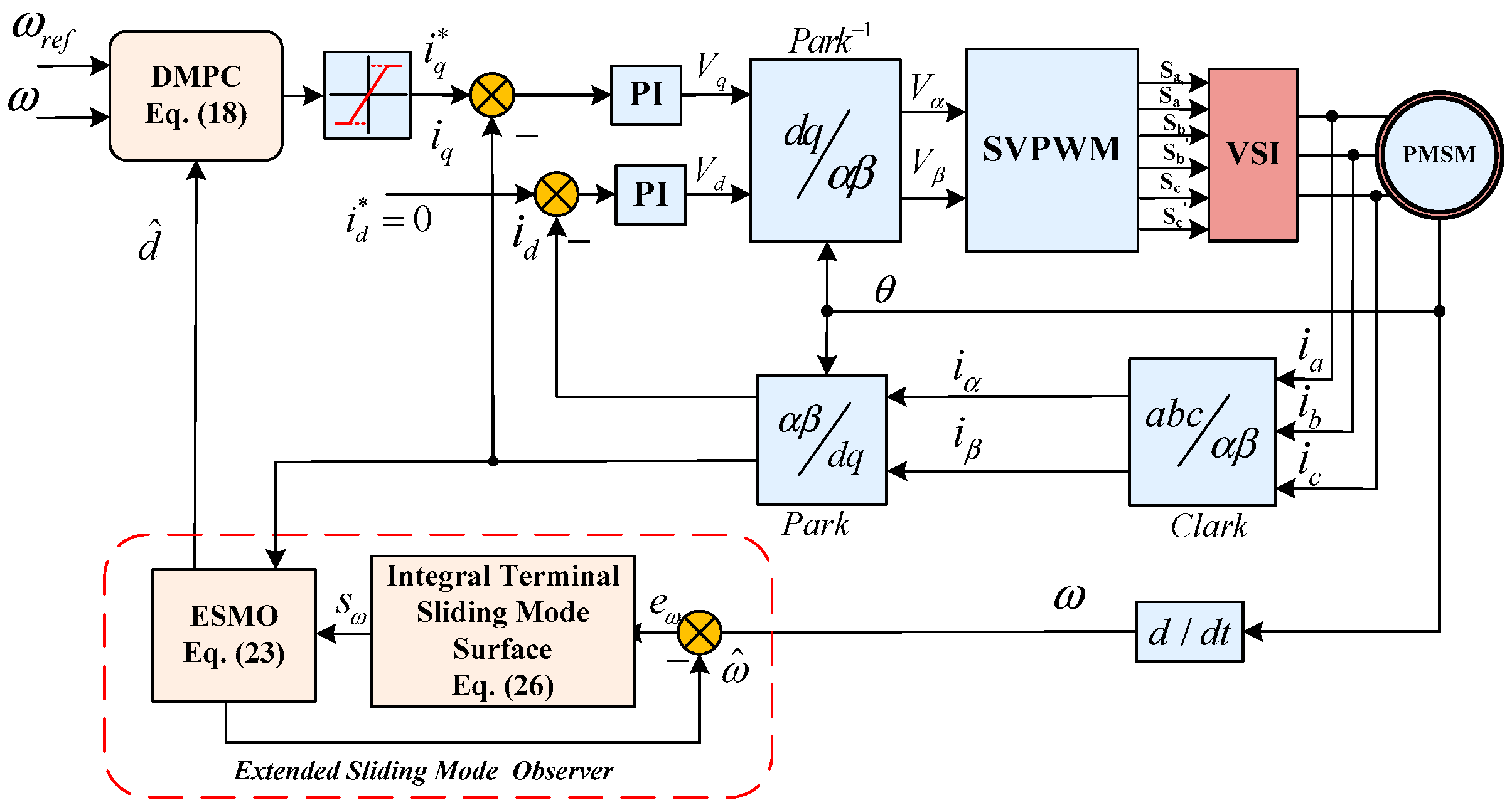
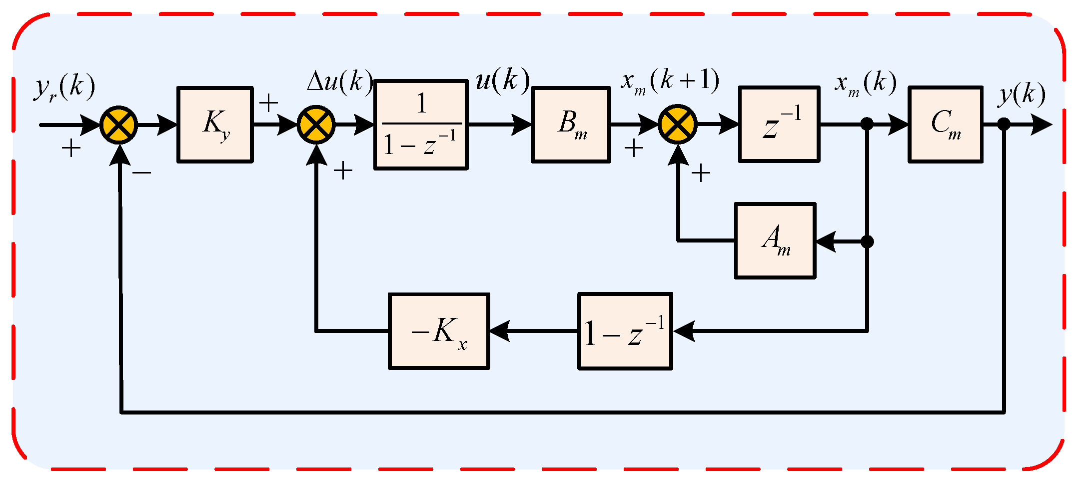
2.2. Design of DMPC for the PMSM

In this paper, a DMPC is designed for the speed loop. To realize computer implementation, an embedded integrator is embedded in the MPC design. The integrator helps reduce the uncertainty of the system in applications and remove the load disturbance torque [14]. In the absence of external disturbances, Equation (2) can be rewritten as follows:

$$\frac{d{\omega }_m}{dt}=\frac{K_t}{J}{i}_q-\frac{B}{J}{\omega }_m$$

(4)

A forward Euler algorithm is applied to Equation (4), such that the discrete-time expression of the predicted rotor mechanical angular velocity at the next sampling instant can be written as follows:

$${\omega }_m(k+1)=(1-\frac{B{T}_s}{J}){\omega }_m(k)+\frac{K_t{T}_s}{J}{i}_q(k)$$

(5)

where T_s is the sampling period.

Thereafter, a discrete state-space model of the PMSM system is used to predict the future outputs online over a defined predicted horizon. In this instance, the predicted output of the system can be expressed as follows:

$$\{\begin{array}{l}{x}_m(k+1)=A_m{x}_m(k)+B_{m}u(k)\\ y_m(k)=C_m{x}_m(k)\end{array}$$

(6)

where, $A_m=(1-\frac{B{T}_s}{J})\begin{array}{cc}& B_m=\frac{K_t{T}_s}{J}\end{array}\begin{array}{cc}& C_m=\end{array}1$, $x_m$ is the state vector of the state-space model, A_m, B_m, and C_m are the coefficients of the state equation, and $y_m$ is the output of the prediction model. In this PMSM speed control system, the state variable $x_m$ is the rotor mechanical angular velocity ${\omega }_m$, and $y_m=x_m$.

Moreover, to realize incremental control in the embedded system, the above state-space equation, i.e., Equation (6), is rewritten as follows:

$$\begin{array}{l}\stackrel{x(k+1)}{\overbrace{\left[\begin{array}{l}\Delta x_m(k+1)\\ y(k+1)\end{array}\right]}}=\stackrel{A}{\overbrace{\left[\begin{array}{ll}{A}_m& 0\\ C_m{A}_m& 1\end{array}\right]}}\stackrel{x(k)}{\overbrace{\left[\begin{array}{l}\Delta x_m(k)\\ y(k)\end{array}\right]}}+\stackrel{B}{\overbrace{\left[\begin{array}{c}{B}_m\\ C_m{B}_m\end{array}\right]}}\Delta u(k)\hfill \\ y(k)=\stackrel{C}{\overbrace{\left[0 1\right]}}\left[\begin{array}{c}\Delta x_m(k)\\ y(k)\end{array}\right]\hfill \end{array}$$

(7)

where

$$\{\begin{array}{l}\Delta x_m(k+1)=x_m(k+1)-x_m(k)\\ \Delta x_m(k)=x_m(k)-x_m(k-1)\\ \Delta u(k)=u(k)-u(k-1)\end{array}$$

$$\begin{array}{l}{x}_m(k+1)-x_m(k)\\ =A_m(x_m(k)-x_m(k-1))+B_m(u(k)-u(k-1))\\ =A_m\Delta x_m(k)+B_m\Delta u(k)\end{array}$$

$$\begin{array}{l}y(k+1)-y(k)\hfill \\ =C_m(x_m(k+1)-x_m(k))=C_m\Delta x_m(k+1)\\ =C_m{A}_m\Delta x_m(k)+C_m{B}_m\Delta u(k)\hfill \end{array}.$$

The new state variables are defined by the differences between the states for any two successive sample instants, and the new state space model equations are obtained.

$$\{\begin{array}{l}x(k+1)=Ax(k)+B\Delta u(k)\hfill \\ y(k)=Cx(k)\hfill \end{array}$$

(8)

where $x(k)={[\Delta x_m{(k)}^{T}y(k)]}^T$, $A=\left[\begin{array}{cc}{A}_m& 0\\ C_m{A}_m& 1\end{array}\right]\begin{array}{cc}& B=\end{array}\left[\begin{array}{l}{B}_m\\ C_m{B}_m\end{array}\right]\begin{array}{cc}& C=\left[\begin{array}{cc}0& 1\end{array}\right]\end{array}$.

It is assumed that at the current sampling instant k (k > 0), the state variable vector x(k) is the current information of the controlled plant, made available through measurement. With the current information of the state variable x(k), the future state variables can be predicted for N_p sampling instants, where N_p is the prediction horizon. According to the state-space model (8), the future state variables can be predicted sequentially using the future control action sequence Δu.

$$\begin{array}{ll}x(k+1|k)& =Ax(k)+B\Delta u(k)\\ x(k+2|k)& =Ax(k+1|k)+B\Delta u(k+1)\\ & =A^{2}x(k)+AB\Delta u(k)+B\Delta u(k+1)\\ & ⋮\\ x(k+N_P|k)& =A^{N_p}x(k)+A^{N_p-1}B\Delta u(k)+A^{N_p-2}B\Delta u(k+1)\\ & +\dots +A^{N_p-N_c}B\Delta u(k+N_c-1)\end{array}$$

(9)

where x(k+m|k) is the predicted state variable at the sampling instant k+m, which is calculated with the current state variable x(k), and N_c (N_c ≤ N_p) is the control horizon.

According to the state-space model (8) and (9), with the state variable information x(k) and the future control action Δu, the predicted output for the next N_p instantscan be predicted.

$$\begin{array}{ll}y(k+1|k)& =CAx(k)+CB\Delta u(k)\\ y(k+2|k)& =C{A}^{2}x(k)+CAB\Delta u(k)+CB\Delta u(k+1)\\ & ⋮\\ y(k+N_P|k)& =C{A}^{N_p}x(k)+C{A}^{N_p-1}B\Delta u(k)+C{A}^{N_p-2}B\Delta u(k+1)\\ & +\dots +C{A}^{N_p-N_c}B\Delta u(k+N_c-1)\end{array}$$

(10)

where y(k+m|k) is the predicted output of the system at the sampling instant k.

The predicted output vectors for the next N_p steps of the samples can then be obtained.

$$Y=Fx(k)+G\Delta U$$

(11)

where

$$\{\begin{array}{l}Y={\left[\begin{array}{cccc}y(k+1|k)& y(k+2|k)& \dots & y(k+N_p)\end{array}\right]}^T\\ \Delta U={\left[\begin{array}{cccc}\Delta u(k)& \Delta u(k+1)& \dots & \Delta u(k+N_c-1)\end{array}\right]}^T\end{array},$$

$$F=\left[\begin{array}{c}CA\\ C{A}^2\\ C{A}^3\\ ⋮\\ C{A}^{N_p}\end{array}\right]G=\left[\begin{array}{ccccc}CB& 0& 0& \dots & 0\\ CAB& CB& 0& \dots & 0\\ C{A}^{2}B& CAB& CB& \dots & 0\\ \hspace{1em}⋮& & & \ddots & \\ C{A}^{N_P-1}B& C{A}^{N_P-2}B& C{A}^{N_P-3}B& \dots & C{A}^{N_P-N_c}B\end{array}\right].$$

According to the augmented state-space model (8), F is a N_p × 2 matrix, G is a N_p × N_c matrix.

2.3. Closed Loop Implementation of DMPC

The purpose of the speed loop optimal control is to determine the optimal incremental control action sequence with a cost function and to ensure that the predicted output of the system is as close as possible to the reference value. With the closed-loop feedback structure, the predictive control action sequence can be corrected in real time. Thus, the DMPC can guarantee the system output to track the command.

The reference vector, which is composed of the reference values, can be expressed as follows:

$$\begin{array}{ll}{Y}_r& =\stackrel{N_p}{\overbrace{{\left[11\dots 1\right]}^T}}{y}_r(k)\\ & =R_y{y}_r(k)\end{array}$$

(12)

where Y_r is the reference vector for the next N_p samples, y_r is the set value for the sampling instant k, R_y is a N_p dimensional unit column vector in this controller.

The cost function J_opt that reflects the control objective is then defined as follows:

$$J_{opt}={(Y_r-Y)}^{T}Q(Y_r-Y)+\Delta U^{T}R\Delta U$$

(13)

where Q is a N_p × N_p positive diagonal weight matrix, and R is a N_c × N_c positive diagonal weight matrix. The first item of the cost function is used to ensure minimum error between the output and the reference value, and the second item of the cost function ensures a lower value of ΔU to suppress the oscillation of the system.

Combining the above with Equation (11), Equation (13) can be written as follows:

$$\begin{array}{l}{J}_{opt}={(Y_r-Fx(k))}^{T}Q(Y_r-Fx(k))\\ -2\Delta U^T{G}^{T}Q(Y_r-Fx(k))+\Delta U^T(G^{T}QG+R)\Delta U\end{array}$$

(14)

Here, the necessary condition for finding the optimal control action sequence ΔU that minimizing J_opt is $\frac{\partial J_{opt}}{\partial \Delta U}=0$. In the absence of constraints, the global optimal control sequence can be obtained by solving this equation as follows:

$$\Delta U={(G^{T}QG+R)}^{-1}{G}^{T}Q(Y_r-Fx(k))$$

(15)

The optimal control action sequence for the next N_c sampling instants can be obtained by minimizing the cost function (13); however, only the first one is applied to the plant as follows:

$$\begin{array}{l}\Delta u(k)=\stackrel{N_c}{\overbrace{[10\dots 0]}}\Delta U\\ =\stackrel{N_c}{\overbrace{[10\dots 0]}}{(G^{T}QG+R)}^{-1}{G}^{T}Q(R_y{y}_r(k)-Fx(k))\\ =K_y{y}_r(k)-K_{xy}x(k)\end{array}$$

(16)

where K_y is the first element of: ${(G^{T}QG+R)}^{-1}{G}^{T}Q{R}_y$ and K_xy is the first element of:${(G^{T}QG+R)}^{-1}{G}^{T}QF$.

The closed-loop system equation can be obtained by substituting Equation (16) into Equation (8).

$$\begin{array}{ll}x(k+1)& =Ax(k)-B{K}_{xy}x(k)+B{K}_y{y}_r(k)\hfill \\ & =(A-B{K}_{xy})x(k)+B{K}_y{y}_r(k)\hfill \end{array}$$

(17)

Because of the special structures of the augmented state-space model parameter matrices A and C, the last column of the matrix F is identical to the unit column vector R_y = [1,1…1]^T. Therefore, K_y is identical to the last element of K_xy, and K_xy can be written as K_xy = [K_x K_y]. To further reflect the closed-loop structure and facilitate computer implementation, control action (16) can be rewritten as follows:

$$\begin{array}{ll}\Delta u(k)& =K_y{y}_r(k)-K_{xy}x(k)\\ & =K_y{y}_r(k)-[K_x{K}_y]{[\Delta x(k)y(k)]}^T\\ & =K_y(y_r(k)-y(k))-K_x\Delta x(k)\end{array}$$

(18)

The matrices K_x and K_y can be computed off-line, and the control action u(k) can be computed on-line using Equation (18). Figure 2 shows the block diagram of the discrete-time MPC system.

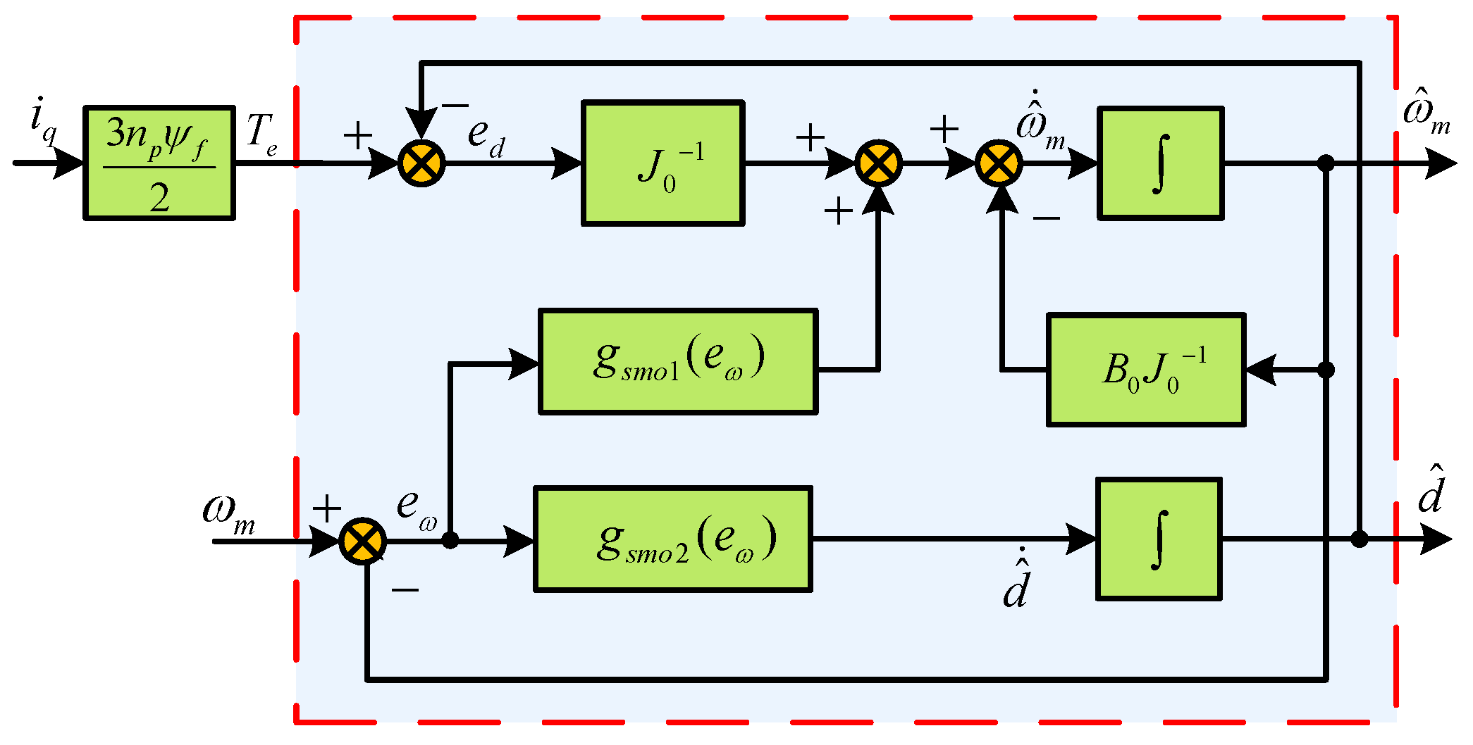
3. Design of Extended Sliding Mode Observer

3.1. DesignofExtended Sliding Mode Observer

Given that the PMSM system will be affected by parameter mismatches and external disturbances during operation, the mathematical model of a PMSM system for practical applications can be expressed as follows:

$$(J_0+\Delta J)\frac{d{\omega }_m}{dt}=T_e-(B_0+\Delta B){\omega }_m-T_L$$

(19)

where J = J₀ + ΔJ, and B = B₀ + ΔB. The parameters B₀ and J₀ are the initial values of the viscous damping coefficient and moment of inertia respectively. They can be determined based on experience and prior knowledge. ΔJ and ΔB are parameter mismatch errors.

Combining Equation (2) with Equation (19), the initial motion equation can be obtained:

$$\{\begin{array}{l}{J}_0\frac{d{\omega }_m}{dt}=T_e-B_0{\omega }_m-d\\ d=\Delta J\dot{\omega }+\Delta B\omega +T_L\end{array}$$

(20)

where d represents the system disturbances including parameter mismatch errors and external load disturbances.

In a PMSM drive system, the electrical time constant is significantly smaller than the mechanical time constant, and the sampling period is very short. The system disturbances change slowly compared to other system status signals in every sampling period of the speed loop. Thus, its first derivative is zero.

$$\dot{d}(t)=0$$

(21)

According to Equation (20), the mechanical angular velocity and the system disturbances $d$ are defined as state variables. The extended state space equation can be expressed as follows:

$$\{\begin{array}{l}\left[\begin{array}{l}{\dot{\omega }}_m^{}\\ \dot{d}\end{array}\right]=\left[\begin{array}{cc}-B_0/J_0& -1/J_0\\ 0& 0\end{array}\right]\left[\begin{array}{l}{\omega }_m\\ d\end{array}\right]+\left[\begin{array}{c}1/J_0\\ 0\end{array}\right]T_e\\ {\omega }_m=\left[10\right]\left[\begin{array}{l}{\omega }_m\\ d\end{array}\right]\end{array}$$

(22)

In the extended state space Equation (22), the mechanical angular velocity ${\omega }_m$ and the disturbance d are regarded as observation targets. Thus, the ESMO can be constructed as follows:

$$\left[\begin{array}{l}{\dot{\widehat{\omega }}}_m^{}\\ \dot{\widehat{d}}\end{array}\right]=\left[\begin{array}{cc}\frac{-B_0}{J_0}& \frac{-1}{J_0}\\ 0& 0\end{array}\right]\left[\begin{array}{l}{\widehat{\omega }}_m\\ \widehat{d}\end{array}\right]+\left[\begin{array}{l}\frac{1}{J_0}\\ 0\end{array}\right]T_e+\left[\begin{array}{l}{g}_{smo1}(e_{\omega })\\ g_{smo2}(e_{\omega })\end{array}\right]$$

(23)

$$\widehat{d}=\Delta \widehat{J}\dot{\omega }+\Delta \widehat{B}\omega +{\widehat{T}}_L$$

(24)

where ${\widehat{\omega }}_m$ is the estimated value of the mechanical angular velocity, $\widehat{d}$ is the estimated value of the system disturbances, $g_{smo}\left(e_{\omega }\right)$ is the sliding mode control function with the mechanical angular velocity observation error $e_{\omega }$. The observation error of the mechanicalangular velocity $e_{\omega }$ and the observation error ofthe system disturbances $e_d$ are defined as follows:

$$\{\begin{array}{l}{e}_{\omega }^{}={\omega }_m^{}-{\widehat{\omega }}_m^{}\\ e_d^{}=d-\widehat{d}\end{array}$$

(25)

The design of the sliding mode surface determines the observation quality of the SMO. The integral sliding mode surface can reduce the chattering of the system and the steady-state error and avoid the analysis of the second derivative. The integral terminal sliding surface is set as follows:

$$s_{\omega }=e_{\omega }+c_{\omega }{\displaystyle {\int }_0^t\mathrm{sgn}(e_{\omega })}d\tau$$

(26)

where $c_{\omega }>0$ is a positive integral coefficient.

In applications, because of the difference calculation in the next part, it is necessary to further suppress the chattering problem. Therefore, a smooth switching function $\vartheta \left(x\right)$ is used instead of the traditional switching function $\mathrm{sgn}\left(x\right)$.

$$\mathrm{sgn}(x)=\vartheta (x)=\frac{x}{\left|x\right|+\delta }$$

(27)

where $\delta >0$ is a constant.

Combining the above with Equations (22), (23), and (25), the equation for the observation error can be written as:

$$\{\begin{array}{l}{\dot{e}}_{\omega }^{}=-\frac{B_0}{J_0}{e}_{\omega }^{}-\frac{1}{J_0}{e}_d-g_{smo1}(e_{\omega })\\ {\dot{e}}_d^{}=-g_{smo2}(e_{\omega })\end{array}$$

(28)

By combining the above equation with Equation (23), the control law of the sliding mode disturbance observer is set as follows.

$$\{\begin{array}{l}{g}_{smo1}(e_{\omega })=c_{\omega }\mathrm{sgn}(e_{\omega })-\frac{B_0}{J_0}{e}_{\omega }+k_1\mathrm{sgn}(s_{\omega })\\ g_{smo2}(e_{\omega })=k_2\mathrm{sgn}(s_{\omega })\end{array}$$

(29)

Proof. 

The Lyapunov function candidate is considered.

$$V=\frac{1}{2}{s}_{\omega }^2$$

(30)

Differentiating V with respect to time t yields the following.

$$\begin{array}{ll}\dot{V}& =s_{\omega }{\dot{s}}_{\omega }\\ & =s_{\omega }(c_{\omega }\mathrm{sgn}(e_{\omega })+{\dot{e}}_{\omega })\\ & =s_{\omega }(c_{\omega }\mathrm{sgn}(e_{\omega })-\frac{B_0}{J_0}{e}_{\omega }-\frac{1}{J_0}{e}_d-g_{smo1}(e_{\omega }))\\ & =s_{\omega }(-\frac{1}{J_0}{e}_d-k_1\mathrm{sgn}(s_{\omega }))\end{array}$$

(31)

where B₀ > 0, and J₀ > 0. To satisfy the finite-time Lyapunov stability theory, the derivative of the Lyapunov function $\dot{V}$ ≤ 0 should be determined. This requires that $s_{\omega }\left[-e_d/J_0-k_{1}sgn\left(s_{\omega }\right)\right]\le 0$, which can be simplified as follows:

$$\{\begin{array}{l}-\frac{e_d}{J_0}+k_1>0 s_{\omega }<0\\ -\frac{e_d}{J_0}-k_1\text{<}0 s_{\omega }\ge 0\end{array}$$

(32)

Therefore, the sliding mode control gain k₁ can be obtained as follows:

$$k_1^{}>\frac{1}{J_0}\left|e_d\right|$$

(33)

This can ensure that the designed observer is stable and that any tracking error trajectory will converge to zero in a finite time.

On the other hand, based on the above ESMO, when the observer trajectory arrives at the sliding surface and remains there, the following condition should be satisfied.

$$\{\begin{array}{l}{s}_{\omega }={\dot{s}}_{\omega }=0\\ e_{\omega }={\dot{e}}_{\omega }=0\end{array}$$

(34)

According to Equations (26), (28), and (29), the following equation can be obtained.

$$\{\begin{array}{l}{\dot{e}}_{\omega }^{}=-\frac{B_0}{J_0}{e}_{\omega }^{}-\frac{1}{J_0}{e}_d-(c_{\omega }\mathrm{sgn}(e_{\omega })-\frac{B_0}{J_0}{e}_{\omega })-k_1\mathrm{sgn}(s_{\omega })\\ {\dot{e}}_d^{}=-k_2\mathrm{sgn}(s_{\omega })\end{array}$$

(35)

The following is obtained by substituting Equation (35) into (34).

$$\{\begin{array}{l}0=-\frac{1}{J_0}{e}_d-k_1\mathrm{sgn}(s_{\omega })\\ {\dot{e}}_d^{}=-k_2\mathrm{sgn}(s_{\omega })\end{array}$$

(36)

Equation (36) can be further simplified as follows.

$$\{\begin{array}{l}{\dot{e}}_d^{}=\frac{k_2}{k_1{J}_0}{e}_d\\ e_d^{}=C_0{e}^{\frac{k_2}{k_1{J}_0}t}\end{array}$$

(37)

where C₀ is a constant, and J₀ > 0. To ensure that the observation error converges to zero, the observer feedback gain must be such that k₂ < 0. According to the above analysis, the system parameters will affect the gain of the observer. By properly adjusting the gain coefficient k₁ and k₂, the observer can achieve a good observation performance. Figure 3 shows a block diagram of the ESMO.  □

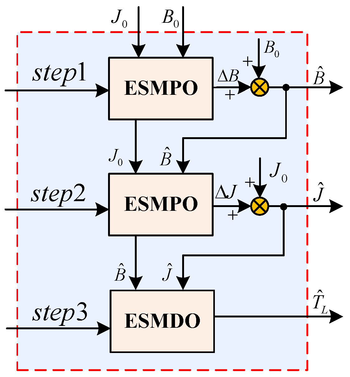
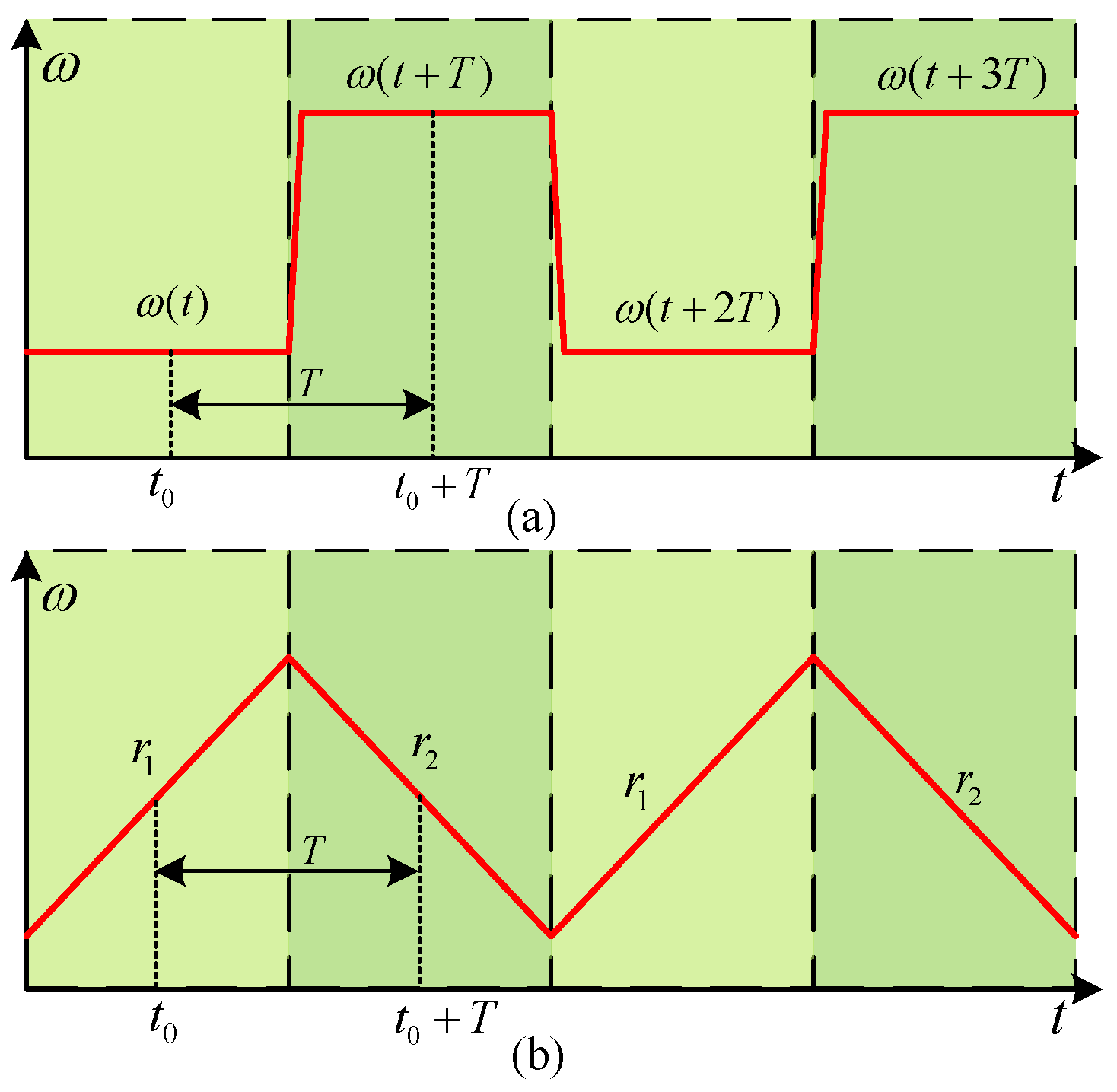
3.2. Parameter Observation Steps

According to Equation (24), the mechanical parameters can be extracted and calculated from the observation disturbances. The mechanical parameters are estimated in three steps [27]. Figure 4 shows the procedure diagram of mechanical parameter estimation. Firstly, the parameter B should be estimated. In the first stage, the PMSM needs to be operated at two different steady-state speeds, and the parameter B can be estimated from the measured velocity information and the observed disturbances. Secondly, the parameter J can be estimated after the parameter B is obtained and updated. In this stage, the PMSM needs to be operated under two different constant accelerations or decelerations, and the parameter J can be estimated from the acceleration or deceleration information and the observed disturbances. Finally, after obtaining and updating the parameters B and J, the ESMO can be regarded as an ESMDO, and the external load torque T_L can be directly estimated from the observation $\widehat{d}$.

An optimal DMPC cannot be established without determining the exact parameters. Therefore, a non-optimal PI speed controller based on a trial-and-error method was used to estimate the mechanical parameters. Although the non-optimal PI controller cannot achieve optimal control performance, only the steady-state information is needed in the parameter estimation process; the non-optimal PI controller has little impact on the parameter estimation process [29]. Figure 5 shows the principle diagram of parameter estimation.

When estimating B, as shown in Figure 5a, the PMSM needs to be operated at two different steady-state speeds, which satisfy the condition ω(t) ≠ ω(t+T) with their accelerations being zero. In Figure 5, T is a predetermined time delay that keeps the system stable for a period of time under the two different speed commands. When the PMSM is operated at the first steady-state speed ω(t) for a period of T, according to Equation (24), the observed disturbance can be obtained as follows:

$$\widehat{d}(t)=\Delta \widehat{J}\dot{\omega }(t)+\Delta \widehat{B}\omega (t)+T_{L0}$$

(38)

The observed disturbance for the second steady-state speed ω(t+T) can be obtained by changing the speed command and keeping it for a period of T as follows:

$$\widehat{d}(t+T)=\Delta \widehat{J}\dot{\omega }(t+T)+\Delta \widehat{B}\omega (t+T)+T_{L0}$$

(39)

The load torque T_L0 of the PMSM system is constant when the PMSM control system is in the steady state. It can be obtained by subtracting Equation (38) from (39).

$$\widehat{d}(t+T)-\widehat{d}(t)=\Delta \widehat{B}\omega (t+T)-\Delta \widehat{B}\omega (t)$$

(40)

Thus, the parameter mismatch error $\Delta \widehat{B}$ can be obtained as follows:

$$\Delta \widehat{B}=\frac{\widehat{d}(t+T)-\widehat{d}(t)}{\omega (t+T)-\omega (t)}$$

(41)

The observed value of the parameter Δ$\widehat{B}$ can be estimated as follows:

$$\widehat{B}=B_0+\Delta \widehat{B}=B_0+\frac{\widehat{d}(t+T)-\widehat{d}(t)}{\omega (t+T)-\omega (t)}$$

(42)

After the parameter B is estimated accurately, the initial value B₀ in Equation (23) can be updated using $\widehat{B}$, and it should satisfy ΔB = B − $\widehat{B}$ = 0.

As shown in Figure 5b, when estimating J, the PMSM needs to be operated at a constant acceleration state r₁ for a period of T. According to Equation (24) and given that ΔB = 0, the observed disturbance can be obtained as follows:

$$\widehat{d}(t)=\Delta \widehat{J}\dot{\omega }(t)+T_{L0}=\Delta \widehat{J}\cdot r_1+T_{L0}$$

(43)

The observed disturbance for the other constant acceleration state r₂ can be obtained by changing the acceleration command and keeping it for a period of T.

$$\widehat{d}(t+T)=\Delta \widehat{J}\dot{\omega }(t+T)+T_{L0}=\Delta \widehat{J}\cdot r_2+T_{L0}$$

(44)

Subtracting Equation (44) from Equation (43) gives the following:

$$\widehat{d}(t+T)-\widehat{d}(t)=\Delta \widehat{J}\cdot r_2-\Delta \widehat{J}\cdot r_1$$

(45)

Thus, the parameter mismatch error $\Delta \widehat{J}$ can be obtained as follows:

$$\Delta \widehat{J}=\frac{\widehat{d}(t+T)-\widehat{d}(t)}{r_2-r_1}$$

(46)

Therefore, the parameter $\widehat{J}$ can be estimated as follows:

$$\widehat{J}=J_0+\Delta \widehat{J}=J_0+\frac{\widehat{d}(t+T)-\widehat{d}(t)}{r_2-r_1}$$

(47)

When the parameters B and J are estimated accurately, the initial B₀ and J₀ in Equation (24) can be replaced by the estimated parameters $\widehat{B}$ and $\widehat{J}$. Now, ΔJ = J − $\widehat{J}$ = 0, and ΔB = B − $\widehat{B}$ = 0. Thus, the disturbance term $\widehat{d}$ can be expressed as follows.

$$\widehat{d}(t)=T_L$$

(48)

The above analysis shows that the proposed ESMO can observe the system disturbances in real-time. In practical applications, the proposed ESMO can be used to optimize the speed controller by estimating the system parameters B and J. Moreover, it can be used to improve the anti-disturbance ability of the system by estimating the external load torque T_L and compensating it online.

4. Simulation and Experimental Results

To demonstrate the effectiveness of the proposed control method, a model of the PMSM system was established using MATLAB/Simulink. Experiments were then conducted on a PMSM drive system. This section reports the results.

Table 1. Parameters of the PMSM.

Parameter	Value
Armature resistance (Rs)	4.3 (Ω)
Armature inductance (Ls)	20.1 (mH)
Torque coefficient (Kt)	0.498 (N∙m/A)
Permanent magnet flux linkage (${\psi }_f$)	0.083 (Wb)
Number of pole pairs (np)	4
Viscous friction coefficient (B)	1.08 × 10−3 (N·m·s/rad)
Rotational inertia (J)	4.7 × 10−4 (Kg∙m2)

lists the actual system parameters of the PMSM.

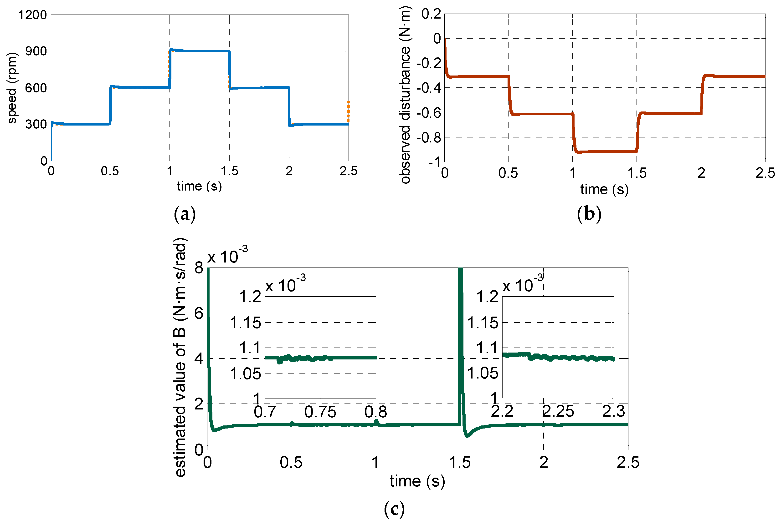
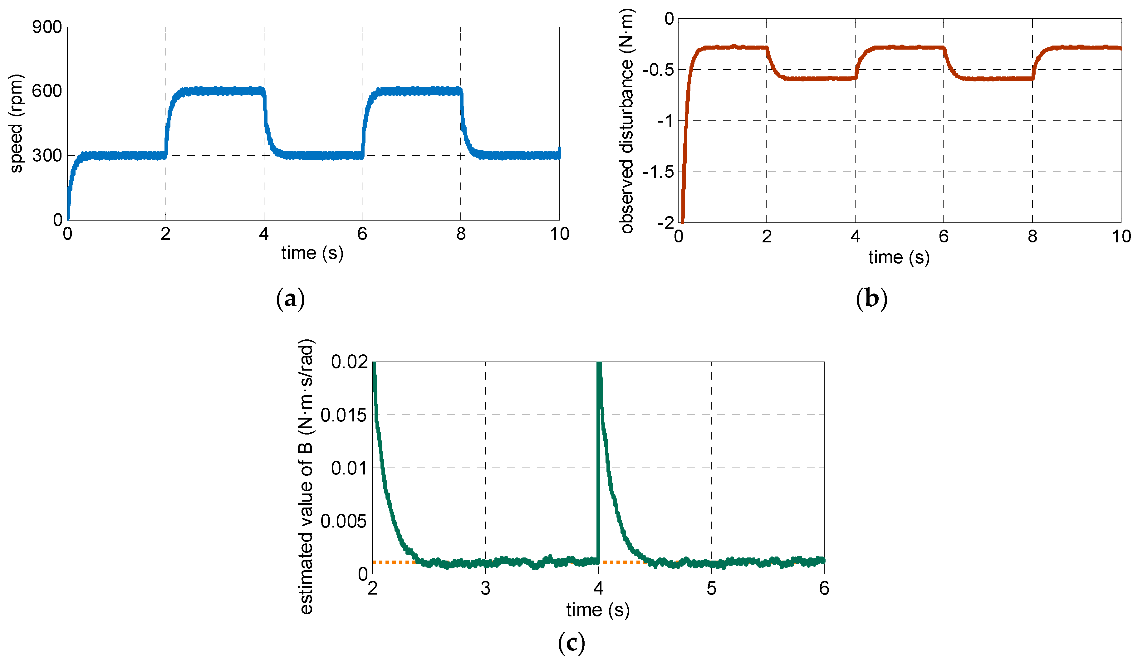
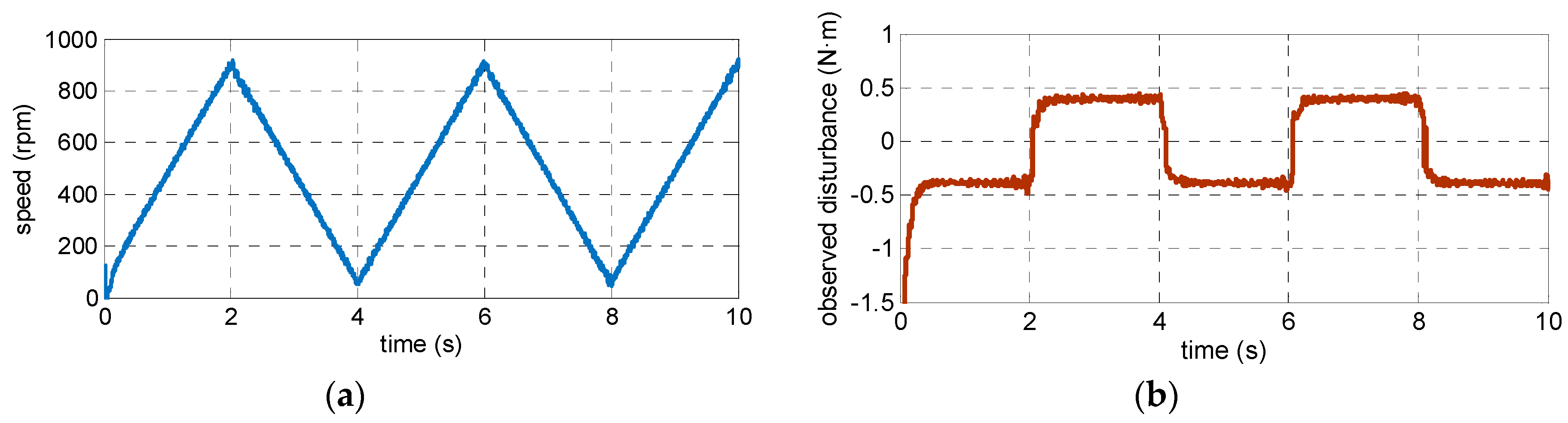
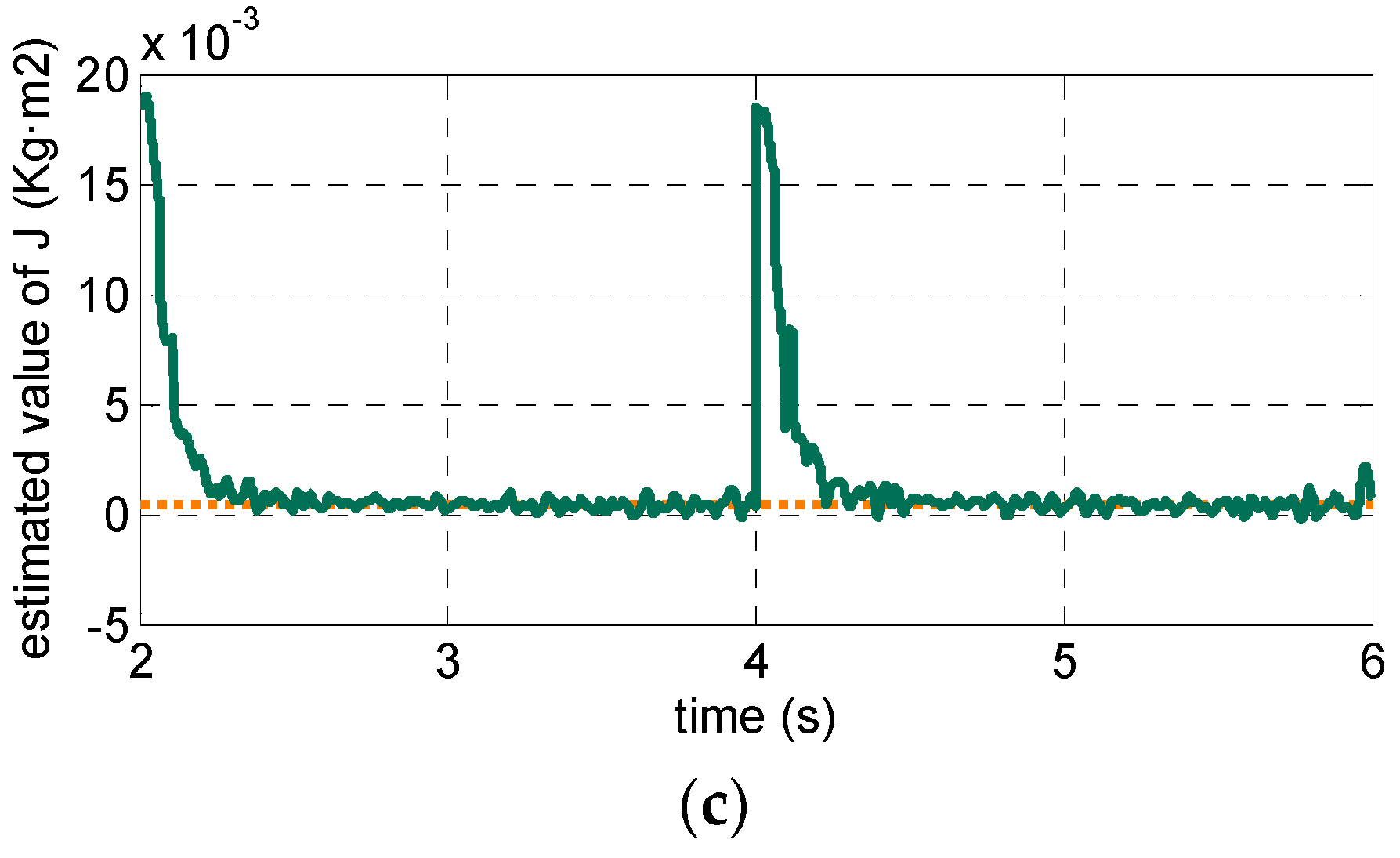
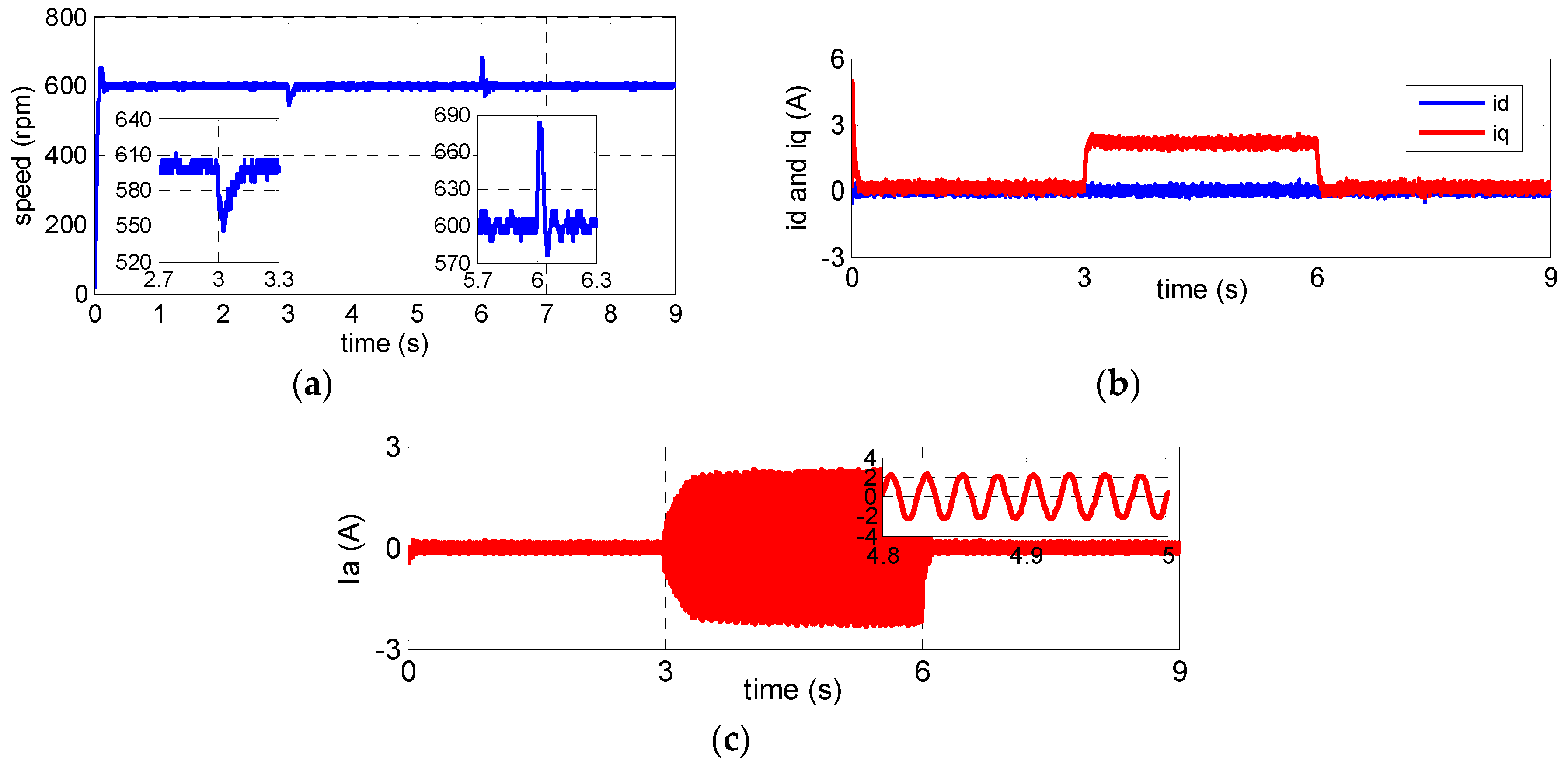
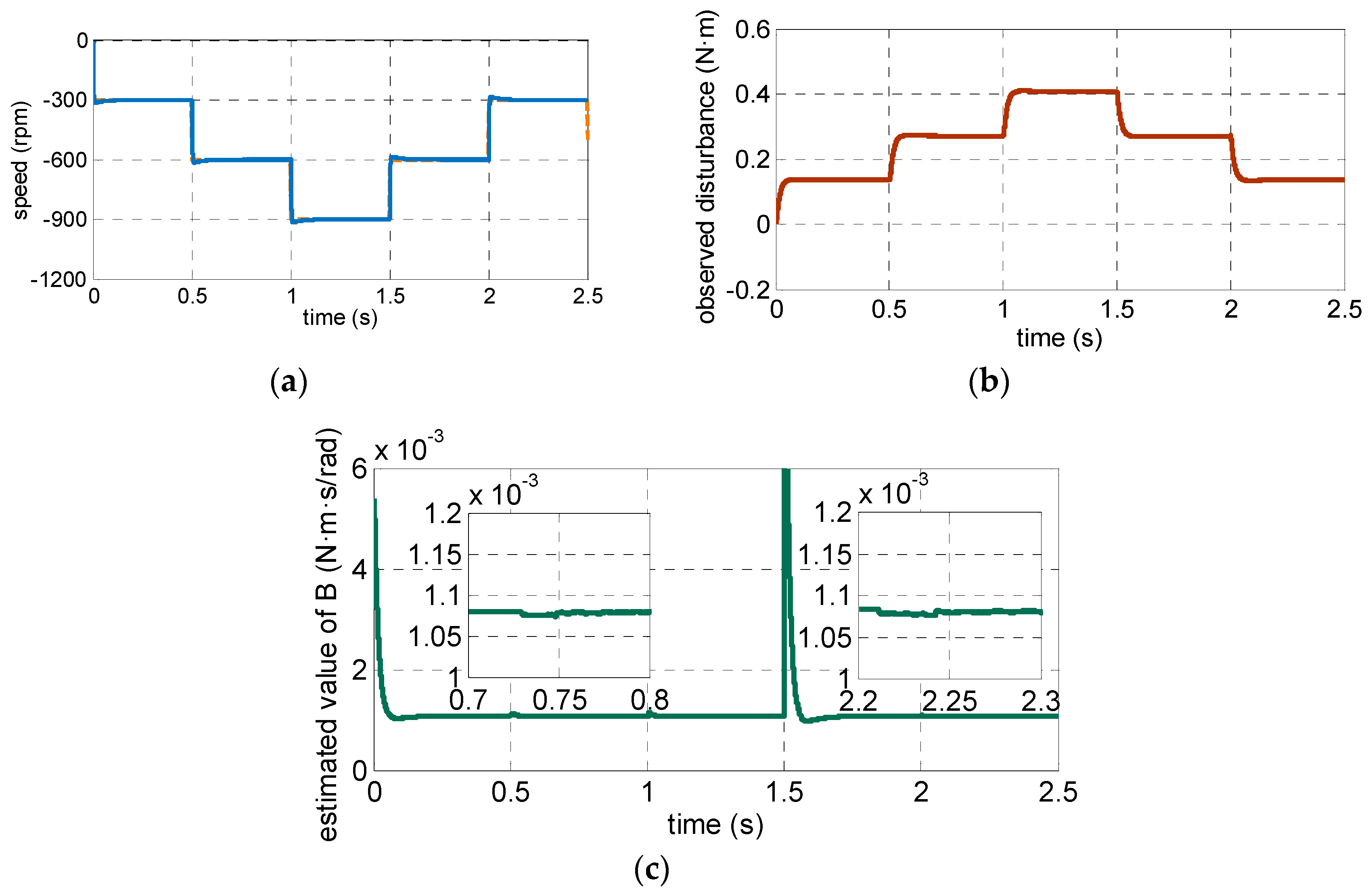
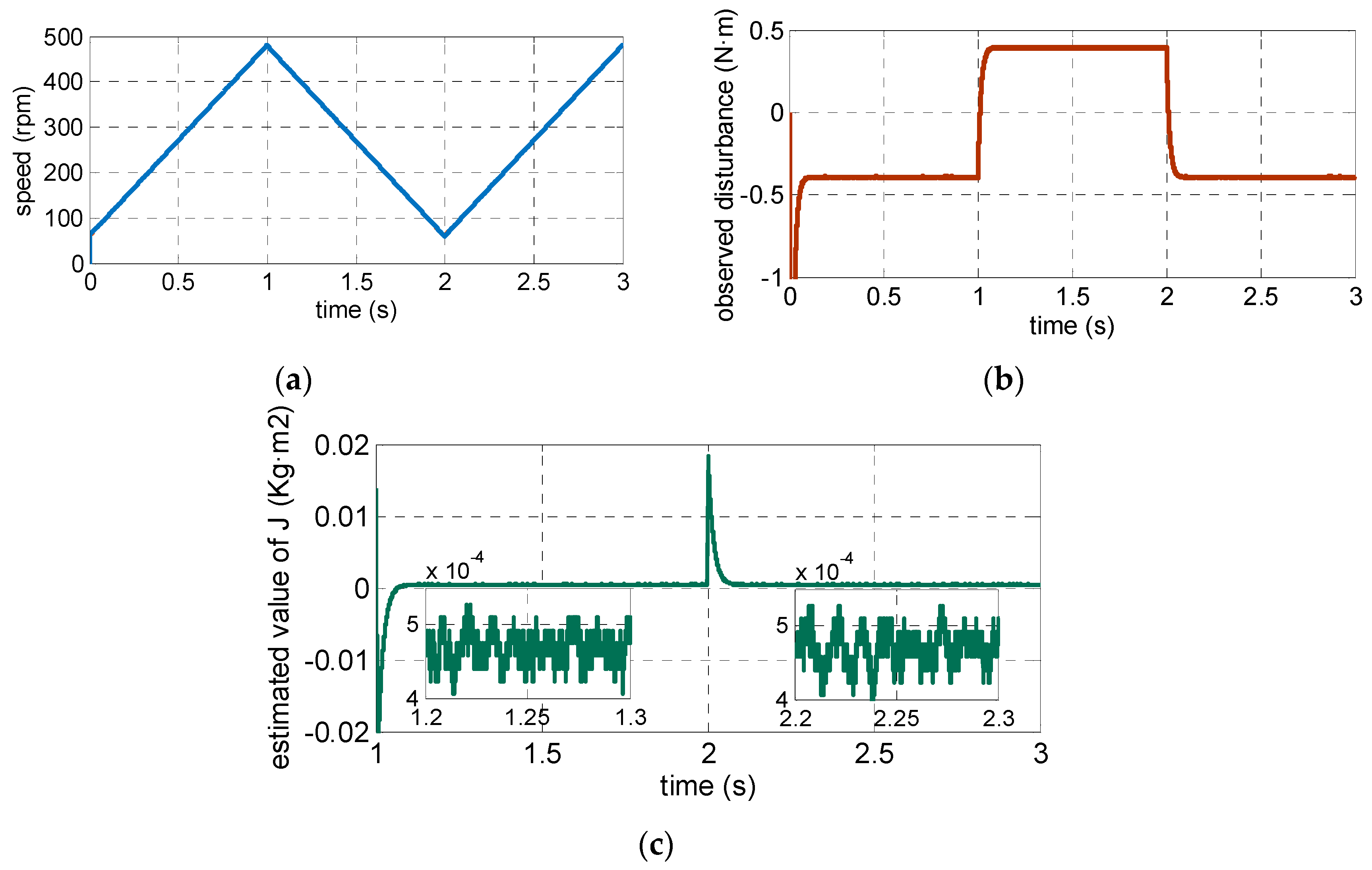
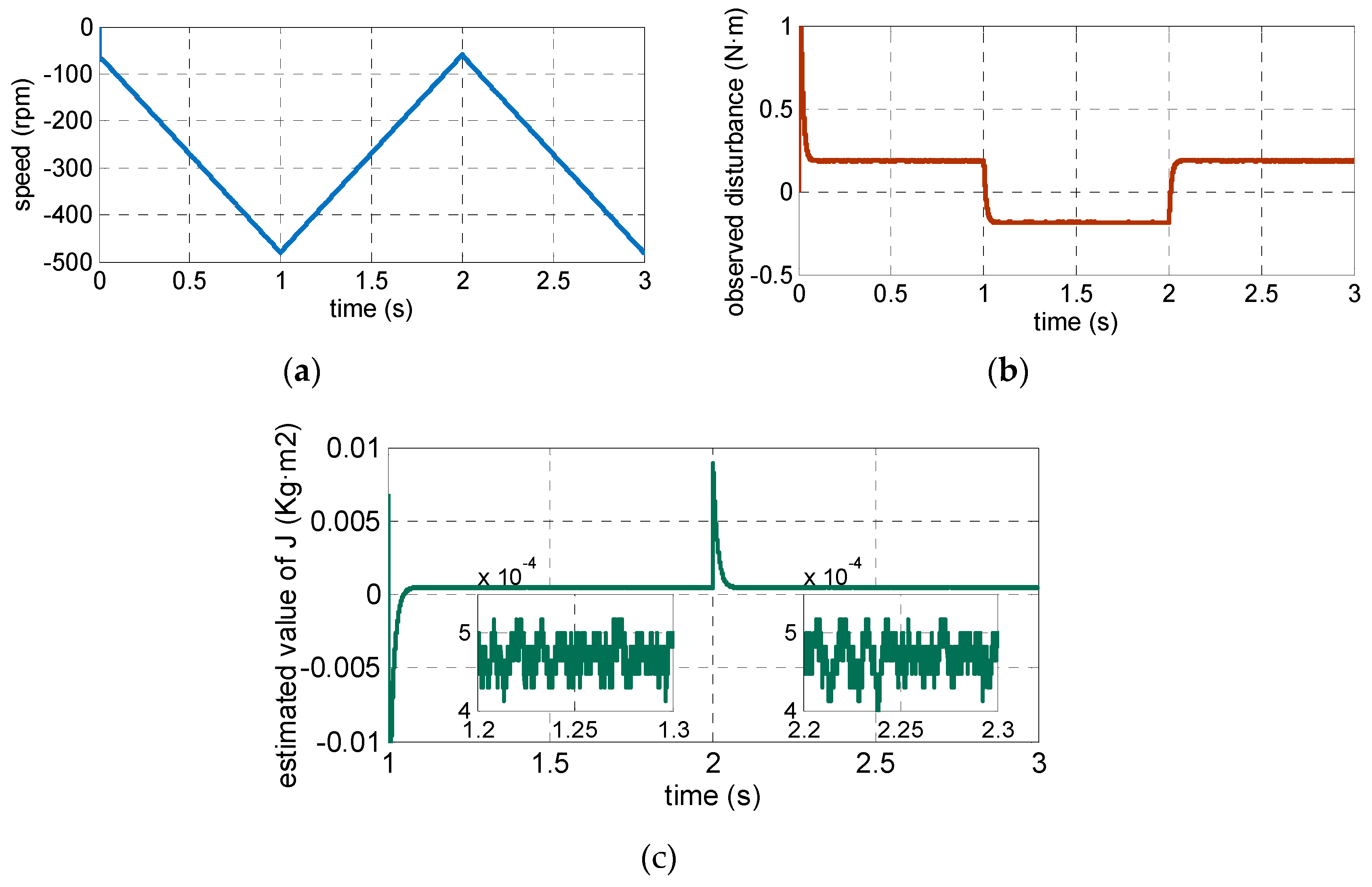
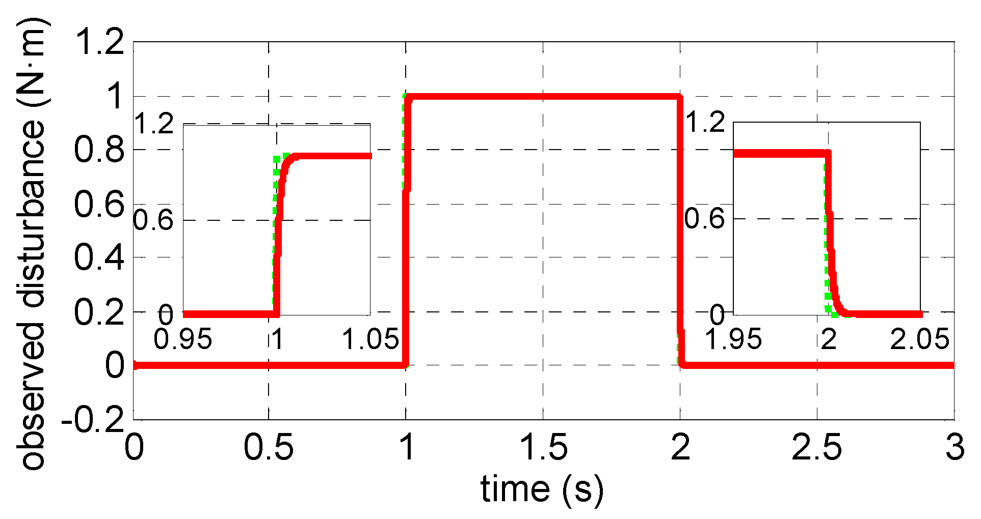
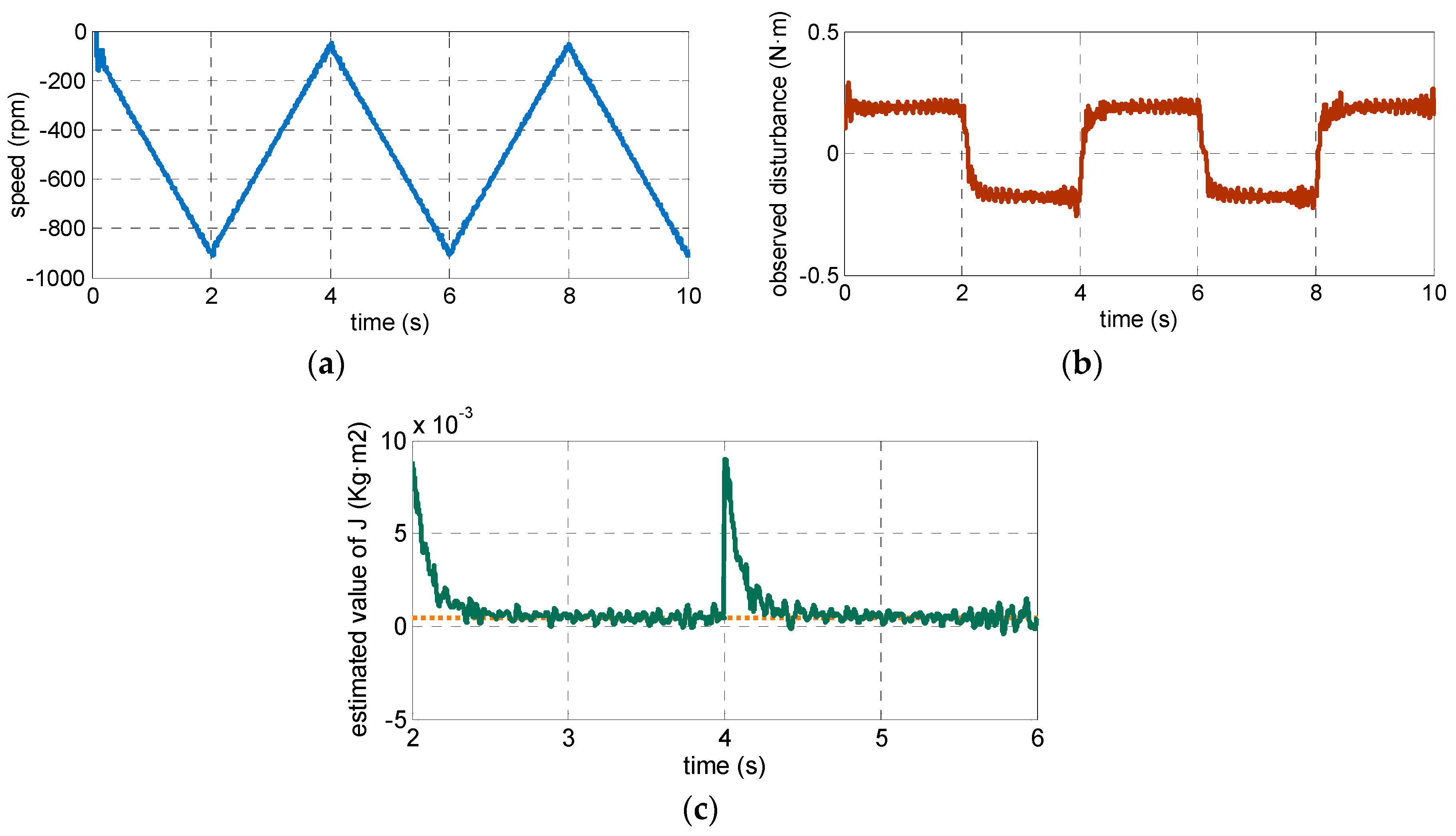
4.1. Simulation Resultsand Analysis

The simulation was conducted under parameter mismatches and a step external load disturbance to test the performance of the proposed ESMO. At the stage of estimating B and J, different initial values B₀ and J₀ are set to the model. Figure 6 and Figure 7 show the observed results of the parameter B. Figure 8 and Figure 9 show the observed results of the parameter J. When estimating T_L, the system applies an external disturbance of 1 N·m at 1 s and then unloads it at 2 s. Figure 10 shows the observed results of the external load disturbance T_L.

As shown in Figure 6 and Figure 7, for different initial values of B₀, the estimated value $\widehat{B}$ can be made to converge to the real value by operating the motor at different stable speeds. As shown in Figure 8 and Figure 9, for different initial values of J₀, the estimated value J can be made to converge to the real value by operating the motor at track different accelerations. After accurately obtaining the mechanical parameters, the proposed observer can be used to observe the external load disturbances. As shown in Figure 10, the proposed ESMO can estimate the external load disturbance precisely and quickly.

The above simulation results show that in the case of parameter mismatches, the proposed observer can estimate and update the observed parameters in real time. Moreover, after updating the parameters, the ESMO can estimate the external disturbance promptly and accurately and provide the observed disturbances as feed-forward compensation for the speed controller.

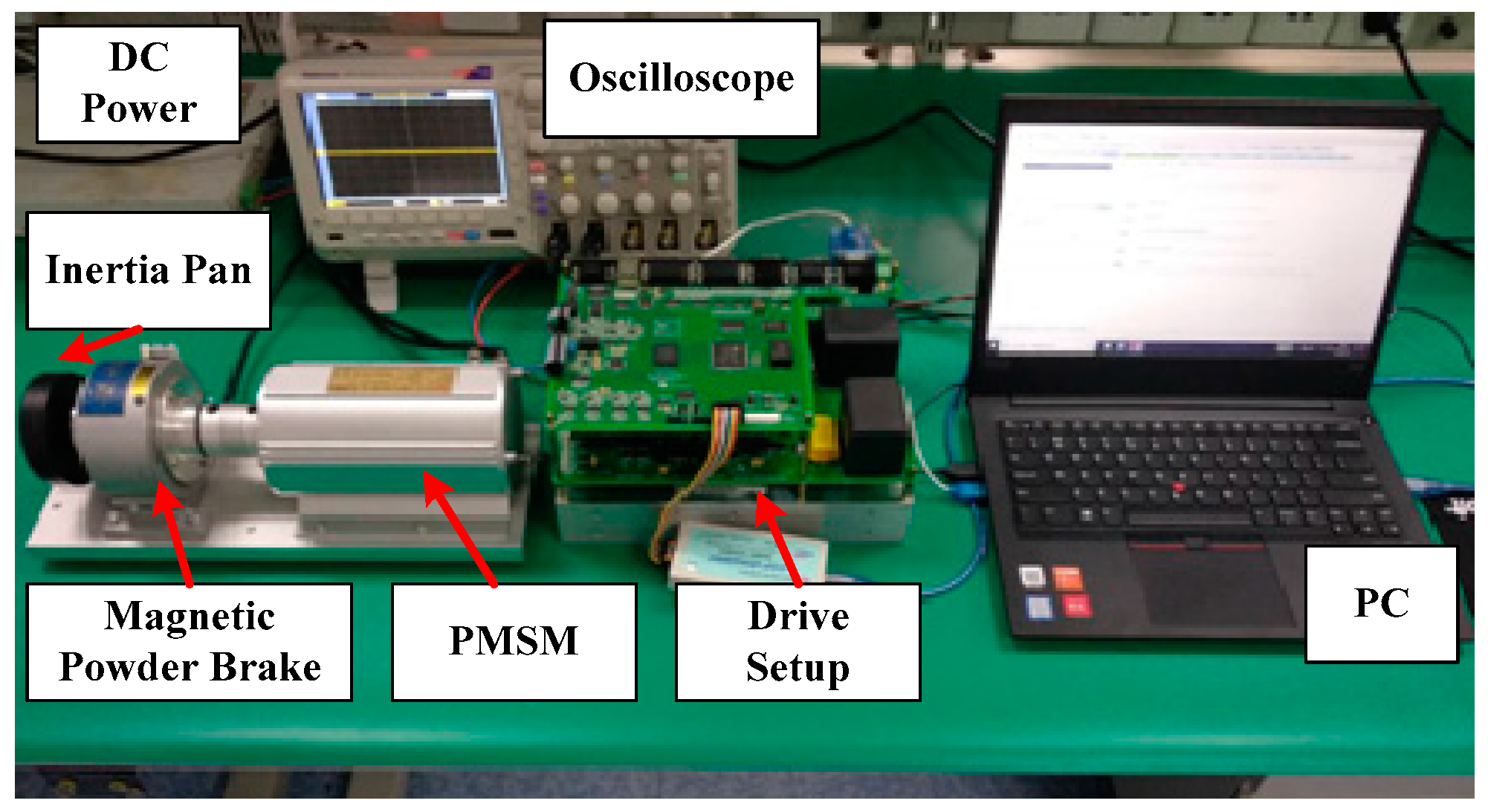
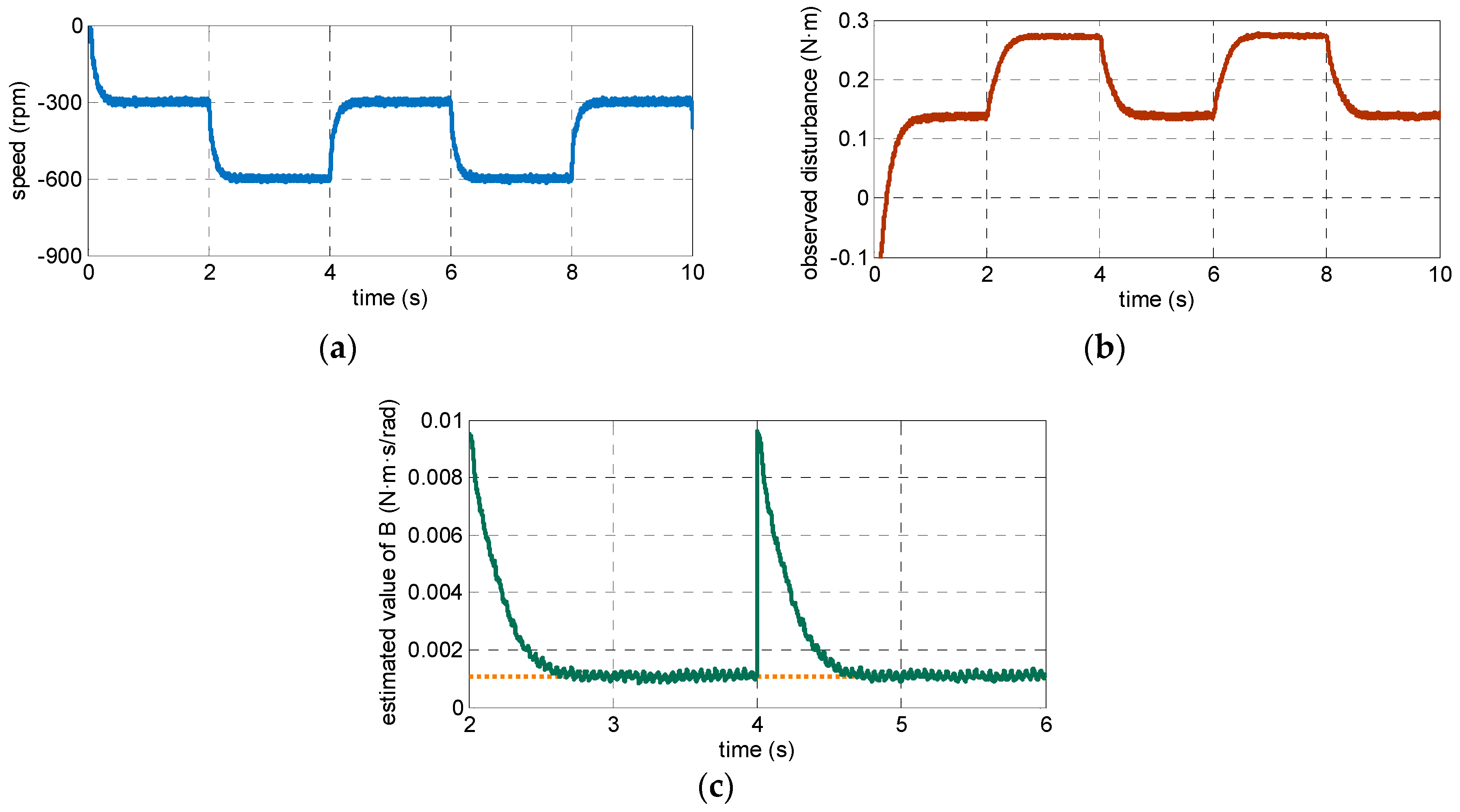
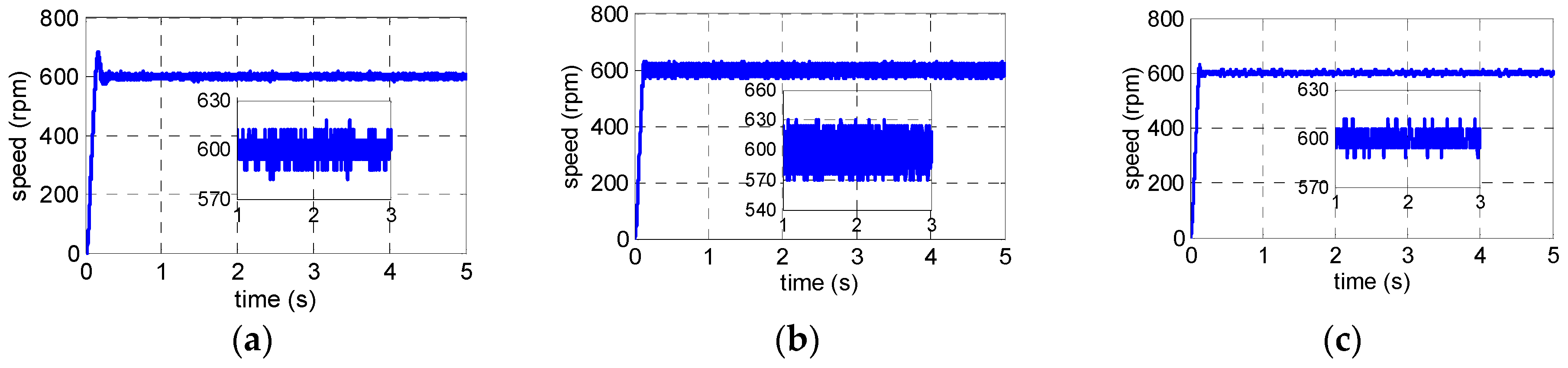
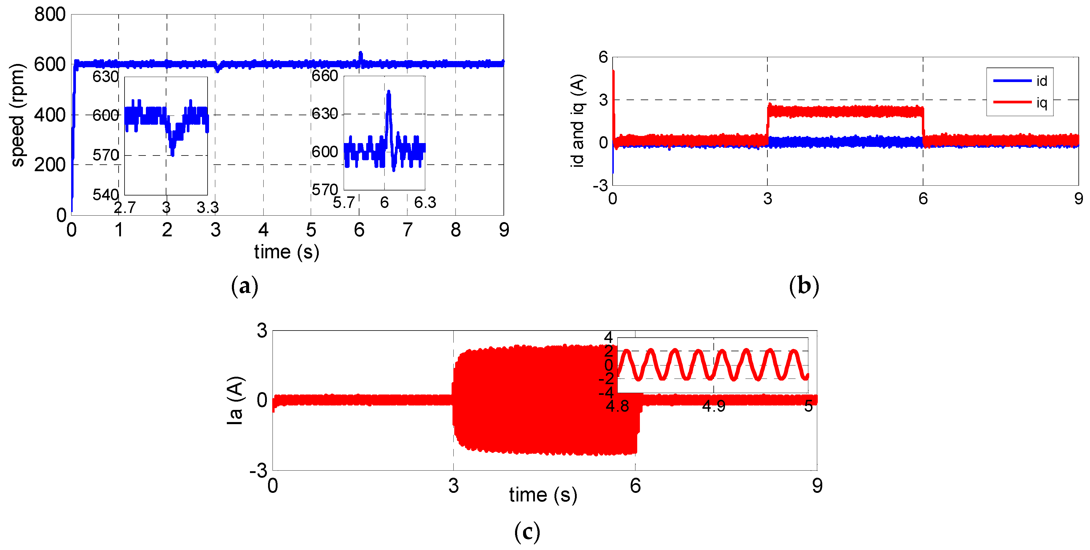
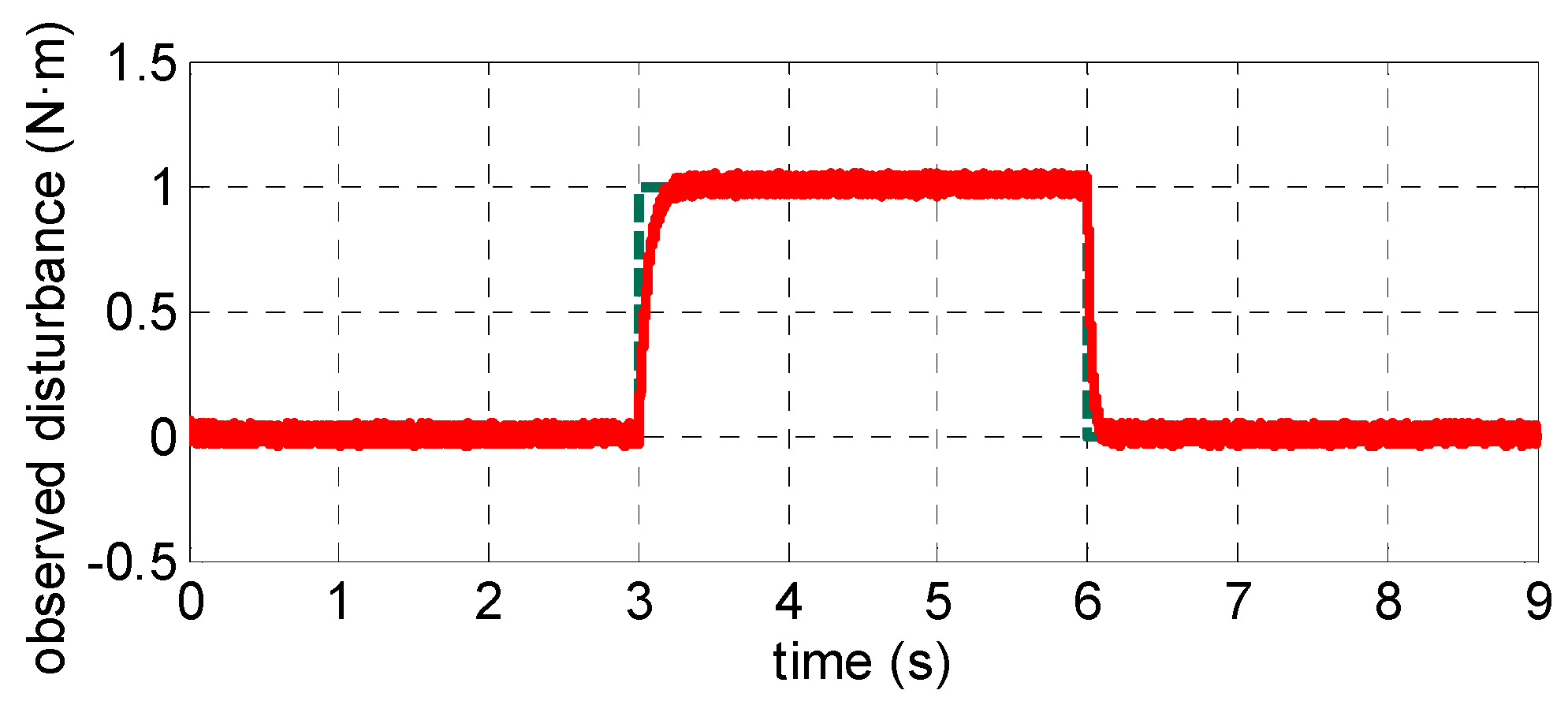
4.2. Experimental Results and Analysis

To further verify the performance of the proposed DMPC with the ESMO method, experiments based on a PMSM drive system are conducted. Figure 11 shows the experimental platform. The proposed control method is realized based on the DSP-TMS320F28335and FPGA-EP3C40F324-based drive setups. The sampling frequency of the speed loop is 1 kHz, and the counterpart frequency of the current loop is 10 kHz.

According to the method described above, the experiment is conducted in three steps. Firstly, the parameter B should be observed and updated. As shown in Figure 12a, the initial value B₀ is set to ten times the true value, i.e., B₀ = 10B, and the PMSM is operated at alternate speeds of 300 and 600 rpm. Figure 12b shows the observed results for the parameter mismatch error ΔB. Figure 12c shows the estimated result of the parameter $\widehat{B}$. As shown in Figure 13a, the initial value B₀ is set to five times the true value, i.e., B₀ = 5B, and the PMSM is operated at alternate speeds of −300 and −600 rpm. Figure 13b shows the observed results for the parameter mismatch error ΔB. Figure 13c shows the estimated results of the parameter $\widehat{B}$.

The parameter J is then observed and updated. As shown in Figure 14a, the initial value J₀ is set to 20 times the true value J, i.e., J₀ = 20J, and the motor is operated to track the acceleration of ±420 rpm/s in the forward direction. Figure 14b shows the observed results for the parameter mismatch error ΔJ. Figure 14c shows the estimated results of the parameter $\widehat{J}$. As shown in Figure 15a, the initial value J₀ is set to ten times the true value J, i.e., J₀ = 10J, and the motor is operated to track the acceleration instruction of ±420 rpm/s in the negative direction. Figure 15b shows the observed results for the parameter mismatch error ΔJ. Figure 15c shows the estimated results of the parameter $\widehat{J}$.

Finally, the observed results of the mechanical parameters can be used to optimize the speed controller and update the observer. When the motor is operated at a given speed of 600 rpm, Figure 16 shows the results under the PI and DMPC method. Then, the system applies an external load disturbance of 1 N at 3 s and then unloads it at 6 s. Figure 17 shows the results obtained using the PI speed controller. Figure 18 shows the results obtained using the DMPC+ESMO method.

As shown in Figure 12, Figure 13, Figure 14 and Figure 15, when the model parameters are mismatched, the estimated value B can be made to converge to the real value by operating the motor at different stable speeds. The estimated value J can be made to converge to the real value by operating the motor to track the different acceleration instructions.

After accurately estimating the mechanical model parameters, the state-space model can be obtained, and the proposed observer can be updated using the estimated parameters. An optimized DMPC with an ESMO can be established for the speed loop.

As shown in Figure 16a, to obtain a faster speed response, the PI method will produce an obvious overshoot in the rising phase. In Figure 16b,c, the DMPC method can achieve a faster speed response with a few overshoots. However, under parameter mismatches, the control performance of the DMPC method will be destroyed. As shown in Figure 16b, the DMPC controller is employed under the condition that the parameter is mismatched with B₀ = 4B and J₀ = 2J. The DMPC method will have a large speed fluctuation near the given speed reference value. The more serious parameter mismatches will lead to greater speed fluctuations and even system instability. As shown in Figure 16c, by using the ESMO to estimate and update parameters, the DMPC+ ESMO method can achieve a better control effect.

As shown in Figure 17, the PI method after updating the parameters can achieve a faster response; however, it results in a significant speed fluctuation when the system is disturbed. To overcome the undesirable speed fluctuation due to the external disturbance, a higher proportional coefficient is required. This will cause a large overshoot in the rise phase. As shown in Figure 18, the DMPC+ESMO method can be employed in the speed loop after updating the parameters. The DMPC controller can achieve an optimal speed control with the optimal control action sequence, and the disturbance compensation technology with the ESMO is applied to improve the anti-disturbance ability and the robustness of the system. A comparison between Figure 17 and Figure 18 shows that when the system loads the external disturbance, the maximum speed fluctuation under the PI method is 54 rpm, whereas the proposed DMPC with the ESMO reduces the maximum speed fluctuation to 24 rpm. The maximum speed fluctuation is reduced by 5%. In Figure 19, the proposed ESMDO accurately and promptly estimates the external load disturbance.

5. Conclusions

In this study, a discrete model predictive controller with an extended sliding mode observer was developed for the speed control system of a PMSM to achieve an optimal speed controlin embedded systems and improve the disturbance rejection performance of the system. The designed controller enabled the system to attain a better dynamic response and reduce speed fluctuations. Moreover, the proposed ESMO could accurately identify the model parameters and the load disturbance of the system. The accurately obtained parameters could be used to update the DMPC, and the observed disturbance is immediately provided as feedback to the DMPC. The simulations and experimental results showed that the DMPC+ESMO method is effective for PMSM speed control systems, enabling better control performance and anti-disturbance ability.

References

1. Su, D.; Zhang, C.; Dong, Y. An Improved Continuous-Time Model Predictive Control of Permanent Magnetic Synchronous Motors for a Wide-Speed Range. Energies 2017, 10, 2051. [Google Scholar] [CrossRef]
2. Liu, J.; Li, H.; Deng, Y. Torque Ripple Minimization of PMSM Based on Robust ILC Via Adaptive Sliding Mode Control. IEEE Trans. Power Electron. 2018, 33, 3655–3671. [Google Scholar] [CrossRef]
3. Liu, X.; Zhang, C.; Li, K.; Zhang, Q. Robust current control-based generalized predictive control with sliding mode disturbance compensation for PMSM drives. ISA Trans. 2017, 71, 542–552. [Google Scholar] [CrossRef] [PubMed]
4. Liu, Y.; Cheng, S.; Ning, B.; Li, Y. Robust model predictive control with simplified repetitive control for electrical machine drives. IEEE Trans. Power Electron. 2019, 34, 4524–4535. [Google Scholar] [CrossRef]
5. Qi, L.; Shi, H. Adaptive position tracking control of permanent magnet synchronous motor based on RBF fast terminal sliding mode control. Neurocomputing 2013, 115, 23–30. [Google Scholar] [CrossRef]
6. Li, S.; Liu, Z. Adaptive Speed Control for Permanent-Magnet Synchronous Motor System with Variations of Load Inertia. IEEE Trans. Ind. Electron. 2009, 56, 3050–3059. [Google Scholar] [CrossRef]
7. Yu, J.; Chen, B.; Yu, H.; Lin, C.; Ji, Z.; Cheng, X. Position tracking control for chaotic permanent magnet synchronous motors via indirect adaptive neural approximation. Neurocomputing 2015, 156, 245–251. [Google Scholar] [CrossRef]
8. Kobayashi, H.; Katsura, S.; Ohnishi, K. An Analysis of Parameter Variations of Disturbance Observer for Motion Control. IEEE Trans. Ind. Electron. 2007, 54, 3413–3421. [Google Scholar] [CrossRef]
9. Wang, T.; Huang, J.; Ye, M.; Chen, J.; Kong, W.; Kang, M.; Yu, M. An EMF Observer for PMSM Sensorless Drives Adaptive to Stator Resistance and Rotor Flux-linkage. IEEE J. Emerg. Sel. Top. Power Electron. 2019, in press. [Google Scholar] [CrossRef]
10. Li, S.; Yang, J.; Chen, W.H.; Chen, X. Generalized Extended State Observer Based Control for Systems with Mismatched Uncertainties. IEEE Trans. Ind. Electron. 2012, 59, 4792–4802. [Google Scholar] [CrossRef]
11. Lin, F.J.; Sun, I.F.; Yang, K.J.; Chang, J.K. Recurrent Fuzzy Neural Cerebellar Model Articulation Network Fault-Tolerant Control of Six-Phase Permanent Magnet Synchronous Motor Position Servo Drive. IEEE Trans. Fuzzy Syst. 2016, 24, 153–167. [Google Scholar] [CrossRef]
12. Liu, H.; Li, S. Speed Control for PMSM Servo System Using Predictive Functional Control and Extended State Observer. IEEE Trans. Ind. Electron. 2012, 59, 1171–1183. [Google Scholar] [CrossRef]
13. Kouro, S.; Cortes, P.; Vargas, R.; Ammann, U.; Rodriguez, J. Model Predictive Control—A Simple and Powerful Method to Control Power Converters. IEEE Trans. Ind. Electron. 2009, 56, 1826–1838. [Google Scholar] [CrossRef]
14. Chai, S.; Wang, L.; Rogers, E. Model predictive control of a permanent magnet synchronous motor with experimental validation. Control Eng. Pract. 2013, 21, 1584–1593. [Google Scholar] [CrossRef]
15. Chai, S.; Wang, L.; Rogers, E. A Cascade MPC Control Structure for a PMSM With Speed Ripple Minimization. IEEE Trans. Ind. Electron. 2013, 60, 2978–2987. [Google Scholar] [CrossRef]
16. Belda, K.; Vosmik, D. Explicit Generalized Predictive Control of Speed and Position of PMSM Drives. IEEE Trans. Ind. Electron. 2016, 63, 3889–3896. [Google Scholar] [CrossRef]
17. Bolognani, S.; Bolognani, S.; Peretti, L.; Zigliotto, M. Design and Implementation of Model Predictive Control for Electrical Motor Drives. IEEE Trans. Ind. Electron. 2009, 56, 1925–1936. [Google Scholar] [CrossRef]
18. Hu, F.; Luo, D.; Luo, C.; Long, Z.; Wu, G. Cascaded Robust Fault-Tolerant Predictive Control for PMSM Drives. Energies 2018, 11, 3087. [Google Scholar] [CrossRef]
19. Wang, C.; Yang, M.; Zheng, W.; Long, J.; Xu, D. Vibration Suppression With Shaft Torque Limitation Using Explicit MPC-PI Switching Control in Elastic Drive Systems. IEEE Trans. Ind. Electron. 2015, 62, 6855–6867. [Google Scholar] [CrossRef]
20. Shoukry, Y.; El-Kharashi, M.W.; Hammad, S. MPC-On-Chip: An Embedded GPC Coprocessor for Automotive Active Suspension Systems. IEEE Embed. Syst. Lett. 2010, 2, 31–34. [Google Scholar] [CrossRef]
21. Song, Z.; Mei, X.; Jiang, G. Inertia identification based on model reference adaptive system with variable gain for AC servo systems. In Proceedings of the 2017 IEEE International Conference on Mechatronics and Automation (ICMA), Takamatsu, Japan, 6–9 August 2017; pp. 188–192. [Google Scholar] [CrossRef]
22. Dybkowski, M. Universal Speed and FluxEstimator for Induction Motor. Power Electron. Drives 2018, 38, 157–169. [Google Scholar] [CrossRef]
23. Liu, Z.; Yang, M.; Xu, D. A novel algorithm for on-line inertia identification via adaptive recursive least squares. In Proceedings of the IECON 2017—43rd Annual Conference of the IEEE Industrial Electronics Society, Beijing, China, 29 October–1 November 2017; pp. 2973–2978. [Google Scholar] [CrossRef]
24. Wang, K.; Chiasson, J.; Bodson, M.; Tolbert, L.M. A nonlinear least-squares approach for identification of the induction motor parameters. IEEE Trans. Autom. Control 2005, 50, 1622–1628. [Google Scholar] [CrossRef]
25. Hong, S.; Lee, C.; Borrelli, F.; Hedrick, J.K. A Novel Approach for Vehicle Inertial Parameter Identification Using a Dual Kalman Filter. IEEE Trans. Intell. Transp. Syst. 2015, 16, 151–161. [Google Scholar] [CrossRef]
26. Niu, L.; Xu, D.; Yang, M.; Gui, X.; Liu, Z. On-line Inertia Identification Algorithm for PI Parameters Optimization in Speed Loop. IEEE Trans. Power Electron. 2015, 30, 849–859. [Google Scholar] [CrossRef]
27. Feng, Y.; Yu, X.; Han, F. High-Order Terminal Sliding-Mode Observer for Parameter Estimation of a Permanent-Magnet Synchronous Motor. IEEE Trans. Ind. Electron. 2013, 60, 4272–4280. [Google Scholar] [CrossRef]
28. Lian, C.; Xiao, F.; Gao, S.; Liu, J. Load Torque and Moment of Inertia Identification for Permanent Magnet Synchronous Motor Drives Based on Sliding Mode Observer. IEEE Trans. Power Electron. 2019, in press. [Google Scholar] [CrossRef]
29. Zhang, X.; Li, Z. Sliding-Mode Observer-Based Mechanical Parameter Estimation for Permanent Magnet Synchronous Motor. IEEE Trans. Power Electron. 2016, 31, 5732–5745. [Google Scholar] [CrossRef]
30. Xu, W.; Jiang, Y.; Mu, C. Novel Composite Sliding Mode Control for PMSM Drive System Based on Disturbance Observer. IEEE Trans. Appl. Supercond. 2016, 26, 1–5. [Google Scholar] [CrossRef]
31. Zhang, X.; Sun, L.; Zhao, K.; Sun, L. Nonlinear Speed Control for PMSM System Using Sliding-Mode Control and Disturbance Compensation Techniques. IEEE Trans. Power Electron. 2013, 28, 1358–1365. [Google Scholar] [CrossRef]
32. Lu, E.; Li, W.; Yang, X.; Xu, S. Composite Sliding Mode Control of a Permanent Magnet Direct-Driven System for a Mining Scraper Conveyor. IEEE Access 2017, 5, 22399–22408. [Google Scholar] [CrossRef]
33. Lyu, M.; Wu, G.; Luo, D.; Rong, F.; Huang, S. Robust Nonlinear Predictive Current Control Techniques for PMSM. Energies 2019, 12, 443. [Google Scholar] [CrossRef]
34. Chiu, C.S. Derivative and integral terminal sliding mode control for a class of MIMO nonlinear systems. Automatica 2012, 48, 316–326. [Google Scholar] [CrossRef]
35. Wang, A.; Jia, X.; Dong, S. A New Exponential Reaching Law of Sliding Mode Control to Improve Performance of Permanent Magnet Synchronous Motor. IEEE Trans. Magn. 2013, 49, 2409–2412. [Google Scholar] [CrossRef]
Figure 1. Structure diagram of the optimized discrete model predictive controller with an extended sliding mode observer.
Energies 12 01857 g001
Figure 2. Block diagram of the discrete-time model predictive control system.
Energies 12 01857 g002
Figure 3. Block diagram of the extended sliding mode observer.
Energies 12 01857 g003
Figure 4. Procedure diagram of mechanical parameter estimation.
Energies 12 01857 g004
Figure 5. Principle diagram of parameter estimation: (a) Estimating B; (b) estimating J.
Energies 12 01857 g005
Figure 6. Simulation results under a speed step of ±300 rpm for B0 = 10B: (a) Measured speed, (b) observed disturbance value for parameter mismatch error ΔB, (c) estimated value of parameter B.
Energies 12 01857 g006
Figure 7. Simulation results under a speed step of ±300 rpm for B0 = 5B: (a) Measured speed; (b) observed disturbance value for parameter mismatch error ΔB; (c) estimated value of parameter B.
Energies 12 01857 g007
Figure 8. Simulation results under an acceleration of ±420 rpm/s for J0 = 20J: (a) Measured speed; (b) observed disturbance value for parameter mismatch error ΔJ; (c) estimated value of parameter J.
Energies 12 01857 g008
Figure 9. Simulation results under an acceleration of ±420 rpm/s for J0 = 10J: (a) Measured speed; (b) observed disturbance value for parameter mismatch error ΔJ; (c) estimated value of parameter J.
Energies 12 01857 g009
Figure 10. Simulation curves of observations based on the extended sliding mode observer (ESMO) for a step disturbance of 1 N·m.
Energies 12 01857 g010
Figure 11. Image of the experimental platform.
Energies 12 01857 g011
Figure 12. Experimental results under alternate speeds of 300 and 600 rpm for B0 = 10B: (a) Measured speed; (b) observed disturbance value for parameter mismatch error ΔB; (c) estimated value of parameter B.
Energies 12 01857 g012
Figure 13. Experimental results under alternate speeds of −300 and −600 rpm for B0 = 5B: (a) Measured speed; (b) observed disturbance value for parameter mismatch error ΔB; (c) estimated value of parameter B.
Energies 12 01857 g013
Figure 14. Experimental results under an acceleration of ±420 rpm/s for J0 = 20J: (a) Measured speed, (b) observed disturbance value for parameter mismatch error ΔJ; (c) estimated value of parameter J.
Energies 12 01857 g014aEnergies 12 01857 g014b
Figure 15. Experimental results under an acceleration of ±420 rpm/s for J0 = 10J: (a) Measured speed; (b) observed disturbance value for parameter mismatch error ΔJ; (c) estimated value of parameter J.
Energies 12 01857 g015
Figure 16. Experimental curves of rotor speed: (a) Under the PI method, (b) under the DMPC method with parameter mismatches by B0 = 4B and J0 = 2J. (c) Under the DMPC and EMSO methods with the parameter estimated value.
Energies 12 01857 g016
Figure 17. Experimental curves of rotor speed with a step disturbance of 1 N·m under the PI method: (a) Rotor speed responses; (b) curves of stator currents in the dq-axis; (c) curves of a-phase stator current.
Energies 12 01857 g017
Figure 18. Experimental curves of rotor speed with a step disturbance of 1 N·m under the DMPC+ESMO method: (a) Rotor speed responses; (b) curves of stator currents in the dq-axis; (c) curves of a-phase stator current.
Energies 12 01857 g018
Figure 19. Experimental curves of observations based on the ESMO for a step disturbance of 1 N·m.
Energies 12 01857 g019