Abstract
This paper discusses nonlinear controller structure design for a synchronous reluctance motor (SynRM). The SynRM is represented with a nonlinear dynamic model. All presented nonlinearities of the SynRM are respected in the controller design procedure. A nonlinear controller policy is used for a SynRM positing system. The nonlinear controller design is based on the chattering alleviation technique for the super-twisted algorithm (STA). The alleviation technique assumes the presence of a fast parasitic dynamic, or fast, actuator. Based on the motor structure, the STA controller is designed only for the mechanical subsystem, where the electrical part presents the parasitic dynamic, and is taken in to account in the chattering suppression procedure. Chattering rejection is based on the STA describing function and harmonic balance equation. The approach allows determination of fast oscillation parameters, such as amplitude and frequency of oscillation. The conditions for the controller parameters’ selection are derived with regard to the given oscillation parameters. The derived conditions cover the stability analysis for the STA controller, as well as the stability condition for current controllers and chattering amplitude minimization. The result is confirmed with an example.
1. Introduction
A synchronous reluctance motor is one of the oldest types of electric motors and uses the principle of reluctance torque to produce electro-mechanical power [1]. Due to its simple construction, ability to withstand the harsh environment, high power to weight ratio, low-cost manufacturing and energy use, the synchronous reluctance motor (SynRM) has become a viable alternative to the other electro-mechanical machines, such as an induction machines (IMs) and permanent-magnet synchronous machines (PMSynMs) [2,3]. If we corroborate with the fact that the availability of the highly efficient permanent magnets have a limited supply ability, wherein the modern technology and economy trend to manufacturing cost reduction, sustainability and environment protection, the SynRM systems have become more and more attractive in diverse applications and gained a lot of attention in the research and engineering communities. The SynRM can be used in different industrial and home applications, as well as a propulsion system in hybrids and electrical vehicles [4]. Various researches over the decade were made to refine the motor torque performance, with a different design of the rotor shape and various multi-phase arrangements [5,6,7,8,9]. There were also many SynRM’s presented, which exploit the synchronous principle of the operation, which are often related to the rotor angle estimation, where the physical sensor is removed [10]. Sensorless application in a SynRM provides higher efficiency and reliability of the system, and is a known approach by other electric drives with an IM and PMSM [11,12].
The mathematical description of a SynRM includes complex dynamics. The complexity is expressed mostly as a nonlinearity of the magnetic characteristics in the direct and quadrature axes [13], where flux linkage characteristics depend on the used currents axes (d-q frame, [1,2,3,4]). The motor drive requires a vector-controlled approach, where the rotor angle information is compulsory. Most recent researches have been done on rotor angle estimation, where the synchronous operation principle was used. Such sensorless approach excludes the operation of the physical sensor, which reduces the possibility of mechanical failure of and simplifies maintenance of the system [10]. The sensorless drive is generally divided into low and high-speed operation modes [10,13,14,15]. The switching boundary between low and high-speed operation is freely selectable, and depends on the motor’s characteristics and application. In the closed-loop system, such switching operation can deteriorate system performance, and is not the objective of the presented work. Feedback controller design for a SynRM involves accurate measurement of the rotor angle, with an installed encoder on the motor shaft. With regard to the well-known dynamic complexity and nonlinearities of the SynMRs, the main objective of the presented work is to design a reliable control law, which can cope with parameter uncertainties and external disturbance rejection. To design a control law that provides the desired closed-loop characteristics in the presence of external disturbance is a very challenging task, leading to interest to deploy robust control paradigms. Among different excellent robust controller paradigms, such as and methods [16], the backstepping approach, and sliding mode control (SMC), which is one of the most effective techniques to handle bounded uncertainty and disturbances [17].
The SMC basic principle of operation is exact keeping of the sliding variable to 0. The sliding variable needs to be properly selected and available in the real-time operation. The SMC needs to be established in an infinite time, and needs to be kept indefinitely, despite the disturbances’ presence or system uncertainties. Considering the above mentioned, the price with deploying a SMC needs to be paid with discontinuous control action, known as the chattering phenomena. The chattering phenomenon is mainly a consequence of the sign function inclusion in the first order SMC (FSCM). Such unwanted phenomena restrict the SMC operation in applications where the high switching operation can cause high wear of the mechanical parts, low control accuracy and high heat losses. Especially, the positioning system with the electromechanical actuator can be a casualty of the harmful chattering phenomena of the FSMC [18,19]. The effective way to attenuate or avoid chattering of the FSMC is to use the Higher Order Sliding Mode (HOSM) technique. [17].
A HOSM approach maintains the same properties as a standard FSMC due to the continuous nature of the controller effort. The main difference between FSCM and HOSM is that the FSCM acts only on the first derivative of the sliding variable , wherein the HOSM acts on higher derivatives of . The sliding motion accrues when the derivatives of , , , and the -th derivative of is a discontinuous function. The order of sliding variable coincides with a relative degree with respect to the control input. The most famous HOSM is a super-twisted sliding mode controller. The super-twisted algorithm (STA) is a second order sliding mode controller (SSMC) [20,21,22,23,24]. In general, the SSMC is capable of ensuring finite time convergence, and leads the system output to zero for the relative degree of two, and additionally, avoids the chattering phenomena for systems with a relative degree of one. The SSMC can deal with the disturbances and uncertainties that are bounded and Lipschitz [20]. The structure of an SSMC-STA is straightforward, and the parameters’ set is correlated directly with the closed-loop dynamic, estimated disturbance and system uncertainty. The main advantage of STA among other orders SSMCs is that the STA does not require , which simplifies the implementation on the real object [17,20,23]. Practical implementations and researches show that the STA can still produce a chattering effect in the vicinity of the sliding surface origin [25]. The main reason for such behavior is an unknown parasitic dynamic or the presence of fast actuators [25,26,27]. To deal with and suppress the unwanted chattering effect, the describing function (DF) methodology for sub-optimal selection of the STA parameters is proposed by Ventura and Fridman [27]. The methodology involves the harmonic balance (HB) equation, where the amplitude and frequency of the chattering phenomena are determined as an intersection point between the Nyquist plot of the linear system and negative reciprocal DF. For the presented problem, the positioning controller design relied on the design of the current and STA positioning controllers, where the sub-optimal solution is presented. The sub-optimal solution is based on the stability proof of the STA and minimization of the amplitude of the chattering phenomena. STA stability analysis is performed on the inspection of the quadratic Lyapunov function candidate proposed by Moreno and Osorio [20], wherein the correlations between the HB solution and the stability property lead to the sub-optimal controller parameter selection. The novel objective functions introduced the inequality for STA stability [20], as well as the HB solution for chattering alleviation. The current controllers are designed for d and q axes, where the d-axis controller parameters are selected in a way that the controller is capable of following slow varying d-current reference signals, and is not subject of the STA chattering suppression with HB.
The structure of the paper is as follows: Section 2 presents the modeling of the SynRM and nonlinear characteristics of the motor. The feedback system is presented with an introduced new variable. In Section 3 the robust current controller’s design is presented, and Section 4 follows with STA positioning controller design. Section 4 introduces the stability analysis of the positioning system, with chattering alleviation based on the DF of STA and HB solution. Section 5 presents the results and evaluation of the positioning system. The conclusion and final thoughts are listed in Section 6.
2. SynRM Modeling
Controller design was based on a mathematical model of the SynRM. Let us consider a mathematical model of SynRM in the reference frame [28]:
where , , and are the dq-voltage, dq-current and resistance, respectively. is the dq-flux linkage due to the dq-current excitation and rotor position . Parameters , , , , and are a motor pole pair, a moment of inertia, viscous friction and load torque, angular velocity and shaft angle, respectively. The system can be divided into electrical and mechanical subsystem (the second and third expression) (1), where the electrical part of the equation represents a connection between electrical and mechanical subsystems. The flux linkage derivatives have a highly nonlinear dependence, which is caused by magnetization characteristic, rotor shape, construction, and position. The nonlinearities of the SynRM taken from [29] are presented in Figure 1, Figure 2 and Figure 3. The used SynRM has 24 skewed slots, with an inside diameter and length of 62 mm and 60 mm. Each phase has 220 turns with phase resistance of 1.3. The rotor is constructed from electric steel, with a diameter and length of 61mm and 60mm, respectively. It has four poles, with three magnetic barriers per each pole. The presented nonlinearities are obtained from 3D finite element modeling and analysis (FEMA) [28,29].
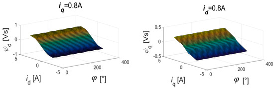
Figure 1.
Flux linkage characteristics and .
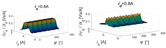
Figure 2.
Partial flux linkage derivative characteristics , .
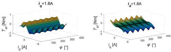
Figure 3.
Electrical torque characteristics , for fixed currents.
From Figure 1, Figure 2 and Figure 3 it is obvious that the SynRM has highly nonlinear behavior, especially Figure 3, which represents an electric torque fluctuation with regard to the rotor shaft position and current values. According to the presented nonlinearities, the feedback controller design needs to ensure the invariance property to a certain class of known bounded uncertainty, which is a proper preference of the SMC technique. The electrical subsystem (1a) was used for the current controller design. The current model will be presented in the next section. For the STA positioning controller design the mechanical subsystem (1a) was used, wherein the STA design, due to simplifications, does not include an electrical subsystem. The dynamic of the electrical subsystem is much higher than the mechanical, therefore, the contribution of the electrical subsystem to the mechanical transient response can be neglected. On the other hand, care needs to be taken, as higher order systems with a relative degree more than two can, nevertheless, cause additional undesirable high-frequency oscillation. The unwanted chattering phenomena with parasitic dynamic are inspected in work [27], where it is shown that the plant with slow dynamic and a relative degree lower, or equal, to two in the presence of a fast actuator or fast parasitic dynamic, can still produce additional oscillation in the vicinity of the origin. The selection of the STA parameters relies on the mechanical subsystem, where the parameters for current controller are based on the inspection of the limit cycle, with regard to the HB solution with an STA describing function. The parameters of the current controller and STA positioning controller were used for high frequency oscillation alleviation.
For the positioning system design governed by the STA, a new variable was introduced:
where are control error, reference, and current angle, respectively. The newly derived model from (1), with introduced variable (2) is
The presented model (3) is the starting point for STA positioning controller design.
3. Current Controller Design
The current controller design covers the design of two separated controllers for each axis separately. The controlled currents ensure the smoother torque characteristic of the SynRM, and are related directly to the connection between both subsystems (1a). The currents’ control is crucial to successful positioning control, and is strongly related to the system dynamic. The design of the -axis controller needs to ensure tracking capability to the static reference signals, where the -axis controller needs to ensure proper dynamics and stability margin. The tracking capability of the -axis does not need to be met, because the controller reference input was governed by the output of the STA positioning controller. The reference for the -axis current controller was selected with regard to the selected torque characteristic and dynamic of the feedback system. The structure of the positioning system with the SynRM is presented in Figure 4.
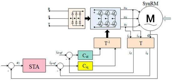
Figure 4.
Feedback controller structure of the super-twisted algorithm (STA) positioning system with synchronous reluctance motor (SynRM).
The dynamic model presented in (4) was used for the current controller’s design. The model is derived from the model given in (1a), where the current derivatives are expressed on the left side of the equation.
The flux linkage partial derivatives can be evaluated as an inductance in both axes.
Assume that , , . The motor inductance can be assessed as:
where the inductances , , with regard to the aforementioned assumption, are zero. The main inductances , have nonlinear characteristics, as presented in Figure 5.
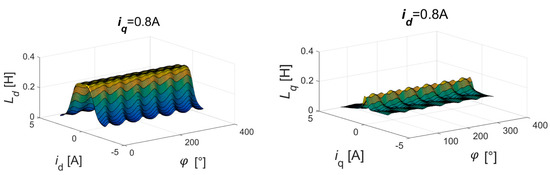
Figure 5.
and inductance characteristics.
A nominal value of and was used for the current controller design. The nominal values were marked as , , , , . With regard to the characteristics presented in Figure 5, it is reasonable to link the STA controller in the -current branch, wherein the -current controller, in regard to the higher provides less fluctuating and constant , which consequently means smoother and higher torque characteristics (1a), Figure 4. The presented model (7) is used for the current controller design.
The classic proportional-integral (PI) structure is used for the current controller.
where is the control error, defined as and , are PI controller parameters. If we put control policy (8) into (7), and after the rearrangement of Equation (7) with the variables and we get:
The final current’s feedback system presented in the state space form, with states , is:
The robustness of the PI controller relies on the Lyapunov stability analysis and introduced positive definite and radially bounded Lyapunov function,
where is vector and . The is positive definite and radially unbounded, where the matrix is equal to:
With regard to the controller structure (8), the assumption is given , , which induces , . To test the stability property of the feedback system, the time derivative of the is calculated as:
where the is equal to:
After the arrangement, the derivative of the is:
where the matrices , and are:
The is donated as a perturbation term of Equation (9). If we assume that the perturbation term is globally bounded by:
for the positive constant than
where is
The system (9) is exponentially stable if . If the perturbation term is neglected , the stability of the system (9) is ensured with , where, from the aforementioned assumption, it follows that , . If the perturbation term is , then matrix is
The controller coefficients need to be selected such that the following holds:
For the current controller design, the simple structure is selected:
where and is a gain coefficient. The current branch is extended to the STA positioning controller, therefore, the selection is inspected, along with the selection of the STA parameters, and does not need a special structure as an . The controller stability with regard to (7) is ensured with the selection . The proper value of will be further related to the chattering alleviation and STA parameters’ selection.
4. Positioning Controller Design
The model presented in Equation (3) was used for the SynMR positioning system design with the STA controller. The STA controller has many positive futures. The STA keeps the same future as an FSMA, which has good rejection capability of the matched known bounded disturbances and uncertainties. Beside the robustness of the STA, the algorithm is simple to implement and is not complex for real-time execution. According to the FSMA on notorious chattering output phenomena, the STA generally produced a continuous output signal. The continuity of the STA output depends on the relative degree of the system, which needs to be of the order of one for completely non-chattering STA output. In the presented positioning controller design, the relative degree of the system with an current controller is equal to three. From the above-mentioned, the chattering phenomena need to be alleviated with proper selection of the controller parameters, which includes STA and controller parameters.
4.1. Super-Twisting Controller Design
A STA modified model in Equation (3) is used:
where
The input of the system is equal to the electric torque produced by the electrical sub-system (1a), with the assumption that the partial flux derivative of angle can be neglected with regard to the flux amount in both d-q axis, , , where the parameter is a known bounded perturbation term.
The introduced sliding variable is
with the first derivative:
where w is a tuning parameter and needs to hold, w > 0. The STA controller has the following form [20,21,26,27]:
where the coefficients , are the tuning parameters and subject to the system stability and chattering alleviation. For a system (16) with sliding variable (19) and STA control law (20), the given feedback system can be expressed as
where the perturbation term is defined as
For the stability analysis of the system (21), the given Lyapunov function is used [20,23]:
The state variable and matrix are
The time derivative of is
where the time derivative of is equal to
After the arrangement, the time derivative of is
where matrices and are
We suppose that the disturbance term is globally bounded by:
where . With the consideration of (23), the second term on the right side of the equation is
Then, the stability of the system is ensured with:
if . Where matrices and are:
The feedback system is globally asymptotically stable with condition and its derivative , if the STA coefficients satisfy the below inequalities:
If we take and from condition (25), the matrix is
For any positive numbers holds that the matrix is strict positive definite, , if the parameters are selected as and . The globally asymptotic stability of the system with the condition (25) is ensured.
4.2. Real Sliding-Mode and Chattering Alleviation
The STA ensures continuous controller output in the case where the relative degree of the system concerning the sliding function is one [30]. For the given control problem with SynRM, it is evident that the aforementioned does not hold. About the simple STA structure and its coefficient conditions (25), some chattering alleviation technique can be used. In our design, the DF technique with limit cycle inspection is used [27,31,32]. The feedback system for the DF approach is presented in Figure 6.
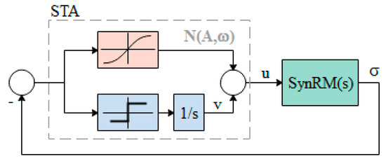
Figure 6.
Describing function technique for super-twisting control system.
The DF technique is used mainly for stability analysis of nonlinear systems and allows us to consider the first-harmonic oscillation. The DF approach uses a presentation of the nonlinear system as a Fourier series, where only the coefficients with the lowest frequency are used. The linear part of the linear presentation of the plant needs to have a low pass characteristic, wherein the Fourier series coefficients with a higher frequency can be neglected [17]. The parameters of the limit cycle can be described as an intersection point of the Nyquist plot of the linear system and negative reciprocal DF which corresponded to the HB [27],
Regarding the STA algorithm (21), the DF of STA [31] is,
where and are amplitude and frequency of the oscillation of the limit cycle. The and represent separately the DF functions of the STA output and first derivative of the output , (21). Where DF functions are,
where the is,
The linear dynamic system can be represented as,
where the parameters derived from (3) and (17) are,
The HB equation (26) for the system (29) and DF (28) is presented as,
The solution of the HB is,
Chattering amplitude can be minimized with proper selection of the parameters , , and . The amplitude can be minimized by introducing:
The solution of the expression (32) gives an optimal value of :
The parameter needs to fulfill the condition (25), where is selected in the manner that the condition (25) holds and the stability of the current controller is ensured.
5. Results
This section indicates the design and parameters’ selection of the position control of the SynRM with regard to the derived conditions. The content of the section is to show the effectiveness of the presented design. The STA efficiency will be compared with some standard approaches, which are based on linear controller and nonlinear FSCM structures. The standard derivation of the proportional-integral-derivative (PID) structure is used for the linear positioning controller. For the given feedback system in Figure 4, the real parameters of the SynRM are presented in (1). Nominal values of the SynRM in Table 1 are selected according to the fixed current and angle values, , , and .

Table 1.
Nominal values of the synchronous reluctance motor (SynRM) parameters.
In order to evaluate the control performance, we have considered three indices, defined as follows,
where , , , are a number of samples, root mean square (RMS) value for motor angle, sliding variable, STA controller output, and current, respectively. For the presented controller design procedure, the value for disturbance terms (12),(23) are presented in Table 2. The parameters are selected regarding the physical limitation of the motor positioning capability and maximal values of the flux linkages and currents values.
Table 2.
Disturbance term parameters.
The parameters for controllers are selected regarding the derived conditions (14),(25),(33). The disturbance terms , (12),(23) in regard to Table 1 and Table 2 are . From the condition (33), they need to be
For the selections the STA parameters are
The selected parameters are presented in Table 3.
Table 3.
Controller parameters.
The experiment is performed with the implemented controllers on the real-time ARM STM32F4xx FPU based system, with sampling time of . The used system is presented in Figure 7.
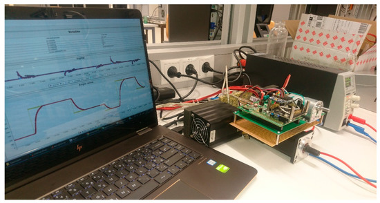
Figure 7.
SynRM positioning system.
Figure 8, Figure 9 and Figure 10 present position control with the STA and current controllers for the parameters given in Table 3.
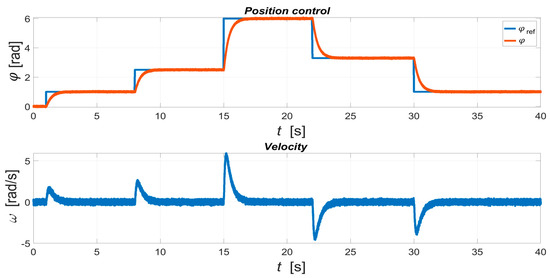
Figure 8.
SynRM positioning control with STA and sub-optimal selection of the controller’s parameters.
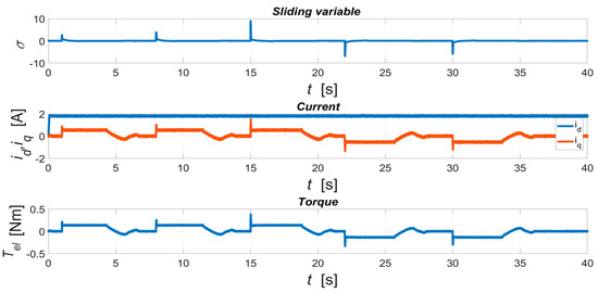
Figure 9.
Sliding variable, current and, on the -axis, electric torque.
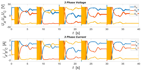
Figure 10.
Three-phase stator voltage and current.
Figure 8, Figure 9 and Figure 10 present the tracking capability on the step reference signal. The step reference signal is filtered with a low-pass filter with a cut-off frequency of 20 Hz. The main purpose of the reference filter is to alleviate the fast transition of the step reference signals, which can produce adverse spikes of the STA controller output. From Figure 8, it can be noticed that the system fulfills all the prescribed design performance. The chattering effect of the nonlinear STA controller cannot be noticed, which means that the current and voltage have a smooth course only contaminated with measurement noise.
Figure 11–13 presents a response to the external load.
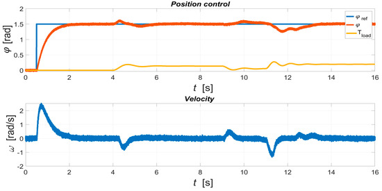
Figure 11.
Position control with response to the external disturbance.
Figure 11, Figure 12 and Figure 13 present the reaction on the external disturbance. From the presented results, it can be concluded that the system is reliable and has proper disturbance rejection capability. The given disturbance line in Figure 11 is estimated from the external unit, and is not measured directly on the system, so the course presented in Figure 11 can vary from real disturbance input.
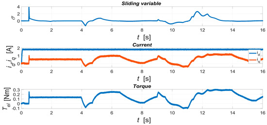
Figure 12.
Sliding variable, currents and electric torque response to the external disturbance.
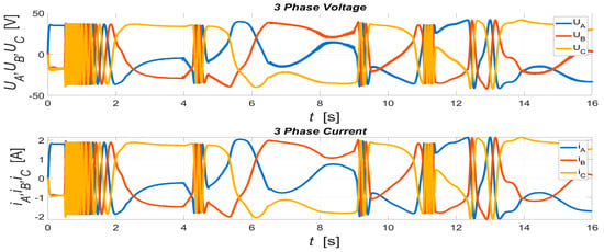
Figure 13.
Three-phase voltage and current response to the external disturbance.
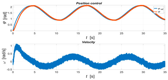
Figure 14.
Tracking capability on the periodic reference signal.
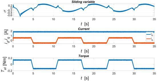
Figure 15.
Sliding variable, currents and electric torque response on the periodic reference signal.
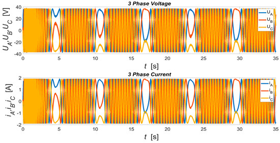
Figure 16.
Three-phase voltage current response on the periodic reference signal.
Figure 14, Figure 15 and Figure 16 present tracking results on the periodic reference signal. The tracking capability on higher frequency reference signals is strictly dependent on the selection of the STA parameters and the system dynamic, where the simple rule holds a higher frequency and higher gain of the STA parameters. Increasing the gain of the STA parameters produced additional chattering by tracking the low-frequency signals. The presented results in Figure 14 use the STA parameters from the previous experiment.
With regard to the sub-optimal selection of the STA and current controller parameters, the competitions are made with a STAcontroller with an unrelated selection of the parameters and , , without condition (33). The parameters , are selected regarding the condition (25), where the stability condition for the current controller is given with . The selected parameters are , , . The second comparison is made with the FSMC and given structure,
where is modulation gain and is , . Sliding variable σ is the same as for STA and STAc controllers. The response to the step reference signal with different controller structures and parameter selection is presented in the next set of figures.

Figure 17.
The response of the STA controller with a sub-optimal selection of the parameters.
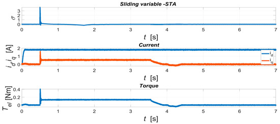
Figure 18.
Sliding variable, currents and electric torque of a sub-optimal STA.
Figure 19 and Figure 20 present the response of the system with a STAc controller, where the standard STA parameters are selected. The selected parameters do not consider the presented chattering alleviation approach.

Figure 19.
The response of the STAcontroller without a sub-optimal selection of the parameters.
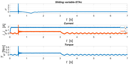
Figure 20.
Sliding variable, currents and electric torque of an STAc controller.
Figure 21 and Figure 22 present the response of the system with an first order sliding mode controller (FSMC) controller.
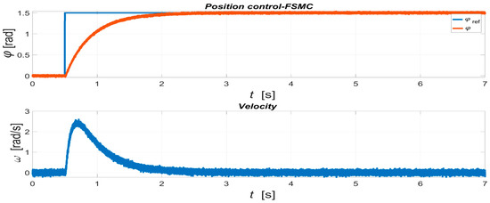
Figure 21.
The response of the FSMC.
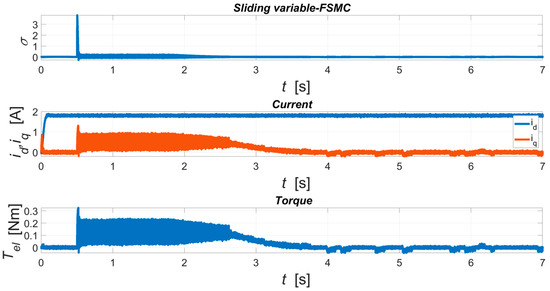
Figure 22.
Sliding variable, currents and electric torque of a FSMC controller.
The Table 4 presents the RMS values of the measured variables , , and u given in (34)–(37).
Table 4.
The root mean square (RMS) values of the variables , , .
From the presented results in Figure 8, Figure 9, Figure 10, Figure 11, Figure 12, Figure 13, Figure 14, Figure 15, Figure 16, Figure 17 and Figure 18 it can be concluded that the presented approach with high-frequency oscillation alleviation gives reliable results according to other tested methods. All the presented methods are capable of steering the control variable to the selected sliding variable. The differences between methods are noticeable in Figure 17, Figure 18, Figure 19, Figure 20, Figure 21 and Figure 22 and Table 4. With regards to the value, it can be concluded that the FSCM slightly overperforms the STA and STAc, which can be endorsed with a bit faster imperceptible response of the control variable (Figure 21). The big difference of the controller efficiency and chattering phenomena can be observed in the controller effort variables Table 4).
The values notified and confirmed the expectation that the STA controller has an, in general, continuous output. Both controller STA, as well as STAc, overperform FSCM. Also, the confirms the same as previously mentioned, with a significant advantage for the STA controller. It can be acknowledged that the un-tuned STA can still produce a high-frequency oscillation, and some techniques for suppression need to be derived and used [27]. The used approach with DF and HB confirms that the chattering phenomena can be suppressed effectively with proper selection of the controller structure and parameters. The expression (33) shows that the parameters of STA and current controller are correlated nonlinearly in a way where kq is correlated reciprocally with parameter and proportional with . The selection of the parameter indicates the relatively high sensitivity to the parameter selection, which means the intersection of the conditions need to be selected (25),(33). The parameters , , are selected in regard to the conditions (25),(33), where sub-optimality is ensured. There exists the possibility of an additional optimization procedure, which can lead to the optimal selection of the controller parameters.
6. Conclusions
A positioning system with a STA controller with a SynRM is presented in this paper. The main objective was to design a positioning system with a SynRM drive and nonlinear STA controller. The methodology introduces chattering suppression based on DF and the HB equation. The key importance of the system is the selection of the controller structure. The presented work introduces a straightforward parameter of the controller, which, interlaced, affects the STA coefficients. The proper selection of the parameters gives satisfactory results of the system tracking capability. For the generalization of the approach, the work can be further extended to the higher order controller structure, which involves more complex conditions for the parameter’s selection. In this case, the optimization procedure would be a necessity. With regard to the mentioned, the used STA controller can be substituted with the generalized version of the STA. The generalized STA also involves linear control terms, which expand the capability of the feedback system in the sense of the robustness on the initial condition and the unknown disturbances and uncertainties. The success of the approach is in agreement with the results on the real system, where it is evident that the presented approach outperforms other similar techniques, such as STAc and FSCM. The time-domain results also confirm the above. The DF with HB is confirmed as an efficient method to analyze the high-frequency oscillation of the feedback system with STA and the SynRM. The derived conditions of the STA with DF-HB also somehow coincides with the standard STA parameter’s selection proposed by Fridman [17], where the proposed method involves, besides robust stability, also high-frequency oscillation suppression.
Author Contributions
R.S. contributed with the design of the controller structure, prepare simulations, experimental results and writing the paper. D.G. contributed with, the feedback linearization, and prepare the stability analysis of the current controller feedback loop. A.C. contributed with, Super Twisted Controller stability analysis and chattering phenomena alleviation based on Describing function approach and Limit cycle analyses. A.S. contributed with Super-Twisted controller design, Describing function approach and derived the suboptimal conditions of the controller’s parameters, real-time implementation the and writing the paper.
Funding
This research received no external funding.
Acknowledgments
The work is supported by the Slovenian Research Agency under the grant number: P2-0065.
Conflicts of Interest
The authors declare no conflicts of interest.
References
- Ogunjuyigbe, A.S.O.; Jimoh, A.A.; Nicolae, D.V.; Obe, E.S. Analysis of synchronous reluctance machine with magnetically coupled three-phase windings and reactive power compensation. IET Electr. Power Appl. 2010, 4, 291–303. [Google Scholar] [CrossRef]
- Anih, L.U.; Obe, E.S.; Abonyi, S.E. Abonyi Modelling and performance of a hybrid synchronous reluctance machine with adjustable Xd/Xq ratio. Electr. Power Appl. IET 2015, 9, 171–182. [Google Scholar] [CrossRef]
- Rakgati, E.; Kamper, M. Torque performance of optimally designed three-and five-phase reluctance synchronous machines with two rotor structures. In Proceedings of the 7th IEEE Africon Conference in Africa, Gaborone, Botswana, 15–17 September 2004; Volume 97, pp. 43–49. [Google Scholar]
- Kumar, R.; Das, S.; Syam, P.; Chattopadhyay, A.K. Review on model reference adaptive system for sensorless vector control of induction motor drives. IET Electr. Power Appl. 2015, 9, 496–511. [Google Scholar] [CrossRef]
- Rakgati, E.T.; Kamper, M.J. Torque Performance of Optimally designed three and Five Phase Reluctance Synchronous Machine. In Proceedings of the 7th IEEE Africon Conference in Africa, Gaborone, Botswana, 15–17 September 2004; Volume 97, pp. 43–49. [Google Scholar]
- Lee, J.H. Optimum Design Criteria for Maximum Torque Density and Minimum Torque Ripple of SynRM According to the Rated Wattage Using Response Surface Methodology. Magn. IEEE Trans. 2009, 45, 1578–1581. [Google Scholar] [CrossRef]
- Sato, S.; Sato, T.; Igarashi, H. Topology Optimization of Synchronous Reluctance Motor Using Normalized Gaussian Network. Magn. IEEE Trans. 2015, 51, 1–4. [Google Scholar] [CrossRef]
- Gilbert, H.B.; Foo, X.Z. Robust Direct Torque Control of Synchronous Reluctance Motor Drives in the Field-Weakening Region. Power Electron. IEEE Trans. 2017, 32, 1289–1298. [Google Scholar]
- Donaghy-Spargo, C.M.; Mecrow, B.C.; Widmer, J.D. Electromagnetic Analysis of a Synchronous Reluctance Motor With Single-Tooth Windings. Magn. IEEE Trans. 2017, 53, 1–7. [Google Scholar] [CrossRef]
- Tuovinen, T.; Hinkkanen, M. Adaptive full-order observer with highfrequency signal injection for synchronous reluctance motor drives. IEEE J. Emerg. Sel. Top. Power Electron. 2014, 2, 181–189. [Google Scholar] [CrossRef]
- Qian, W.; Zhang, X.; Fanning, J.; Hua, B.; Dingguo, L.; Cheng, B. Using High-Control-Bandwidth FPGA and SiC Inverters to Enhance High-Frequency Injection Sensorless Control in Interior Permanent Magnet Synchronous Machine. IEEE Access 2018, 6, 42454–42466. [Google Scholar] [CrossRef]
- Wang, G.; Li, Z.; Zhang, G.; Yu, Y.; Xu, D. Quadrature PLL-Based High-Order Sliding-Mode Observer for IPMSM Sensorless Control With Online MTPA Control Strategy. IEEE Trans. Energy Convers. 2013, 28, 214–224. [Google Scholar] [CrossRef]
- Morales-Caporal, R.; Pacas, M. Encoderless predictive direct torque control for synchronous reluctance machines at very low and zero speed. IEEE Trans. Ind. Electron. 2008, 55, 4408–4416. [Google Scholar] [CrossRef]
- Hanamoto, T.; Ghaderi, A.; Harada, H.; Tsuji, T. Sensorless Speed Control of Synchronous Reluctance Motor Using a Novel Flux Estimator Based on Recursive Fourier Transformation. In Proceedings of the IEEE International Conference on Industrial Technology, Victoria, Australia, 10–13 February 2009; pp. 1–9. [Google Scholar]
- Zarchi, H.A.; Markadeh, G.R.A.; Soltani, J. Direct torque and flux regulation of synchronous reluctance motor drives based on input-output feedback linearization. Energy Convers. Manag. 2010, 5, 71–80. [Google Scholar] [CrossRef]
- Zhou, K.; Doyle, J. Essentials of Robust Control; Prentice-Hall: Upper Saddle River, NJ, USA, 1998. [Google Scholar]
- Shtessel, Y.; Edwards, C.; Fridman, L.; Levant, A. Sliding Mode Control and Observation; Birkhäuser: Basel, Switzerland, 2014. [Google Scholar]
- Utkin, V.; Guldner, J.S. Sliding Mode Control in Electromechanical Systems; CRC Press: Boca Raton, FL, USA, 1999. [Google Scholar]
- Rivera, J.D.; Mora-Soto, C.; Ortega, S.; Raygoza, J.J.; De La Mora, A. Super-twisting control of induction motors with core loss. In Proceedings of the 11th International Workshop on Variable Structure Systems (VSS), Mexico City, Mexico, 26–28 June 2010; pp. 428–433. [Google Scholar]
- Moreno, J.A.; Osorio, M. Strict Lyapunov functions for the super-twisting algorithm. IEEE Trans. Autom. Control 2012, 57, 1035–1040. [Google Scholar] [CrossRef]
- Evangelista, C.; Puleston, P.; Valenciaga, F.; Fridman, L. Lyapunov-designed super-twisting sliding mode control for wind energy conversion optimization. IEEE Trans. Ind. Electron. 2013, 60, 538–545. [Google Scholar] [CrossRef]
- Chalanga, A.; Kamal, S.; Fridman, L.; Bandyopadhyay, B.; Moreno, J.A. Implementation of super-twisting control: Super-twisting and higher order sliding-mode observer-based approaches. IEEE Trans. Ind. Electron. 2016, 63, 3677–3685. [Google Scholar] [CrossRef]
- Morfin, O.A.; Castañeda, C.E.; Valderrabano-Gonzalez, A.; Hernandez-Gonzalez, M.; Valenzuela, F.A. A Real-Time SOSM Super-Twisting Technique for a Compound DC Motor Velocity Controller. Energies 2017, 10, 1286. [Google Scholar] [CrossRef]
- Kali, Y.; Ayala, M.; Rodas, J.; Saad, M.; Doval-Gandoy, J.; Gregor, R.; Benjelloum, K. Current Control of a Six-Phase Induction Machine Drive Based on Discrete-Time Sliding Mode with Time Delay Estimation. Energies 2019, 12, 170. [Google Scholar] [CrossRef]
- Utkin, V. Discussion aspects of high-order sliding mode control. IEEE Trans. Autom. Control 2016, 61, 829–833. [Google Scholar] [CrossRef]
- Ventura, U.P.; Fridman, L. When is it reasonable to implement the discontinuous sliding-mode controllers instead of the continuous ones? Frequency domain criteria. Int. J. Robust Nonlinear Control 2019, 29, 810–828. [Google Scholar] [CrossRef]
- Ventura, U.P.; Fridman, L. Design of super-twisting control gains: A describing function based methodology. Automatic 2019, 99, 175–180. [Google Scholar] [CrossRef]
- Stumberger, G.; Stumberger, B.; Dolinar, D. Identification of linear synchronous reluctance motor parameters. IEEE Trans. Ind. Appl. 2004, 40, 1317–1324. [Google Scholar] [CrossRef]
- Igrec, D.; Chowdhury, A.; Štumberger, B.; Sarjaš, A. Robust tracking system design for a synchronous reluctance motor—SynRM based on a new modified bat optimization algorithm. Appl. Soft Comput. 2018, 69, 568–584. [Google Scholar] [CrossRef]
- Golkani, M.A.; Koch, S.; Reichhartinger, M.; Horn, M. A novel saturated super-twisting algorithm. Syst. Control Lett. 2018, 119, 52–56. [Google Scholar] [CrossRef]
- Boiko, I.; Fridman, L. Analysis of chattering in continuous sliding mode controllers. IEEE Trans. Autom. Control 2005, 50, 1442–1446. [Google Scholar] [CrossRef]
- Ventura, U.P.; Fridman, L. Chattering measurement in SMC and HOSMC. In Proceedings of the 14th International Workshop on Variable Structure Systems, Nanjing, China, 1–4 June 2016; pp. 108–113. [Google Scholar]
© 2019 by the authors. Licensee MDPI, Basel, Switzerland. This article is an open access article distributed under the terms and conditions of the Creative Commons Attribution (CC BY) license (http://creativecommons.org/licenses/by/4.0/).