A Comparative Computational Fluid Dynamic Study on the Effects of Terrain Type on Hub-Height Wind Aerodynamic Properties


Abstract
1. Background
2. Data and Methodology
3. Results and Discussion
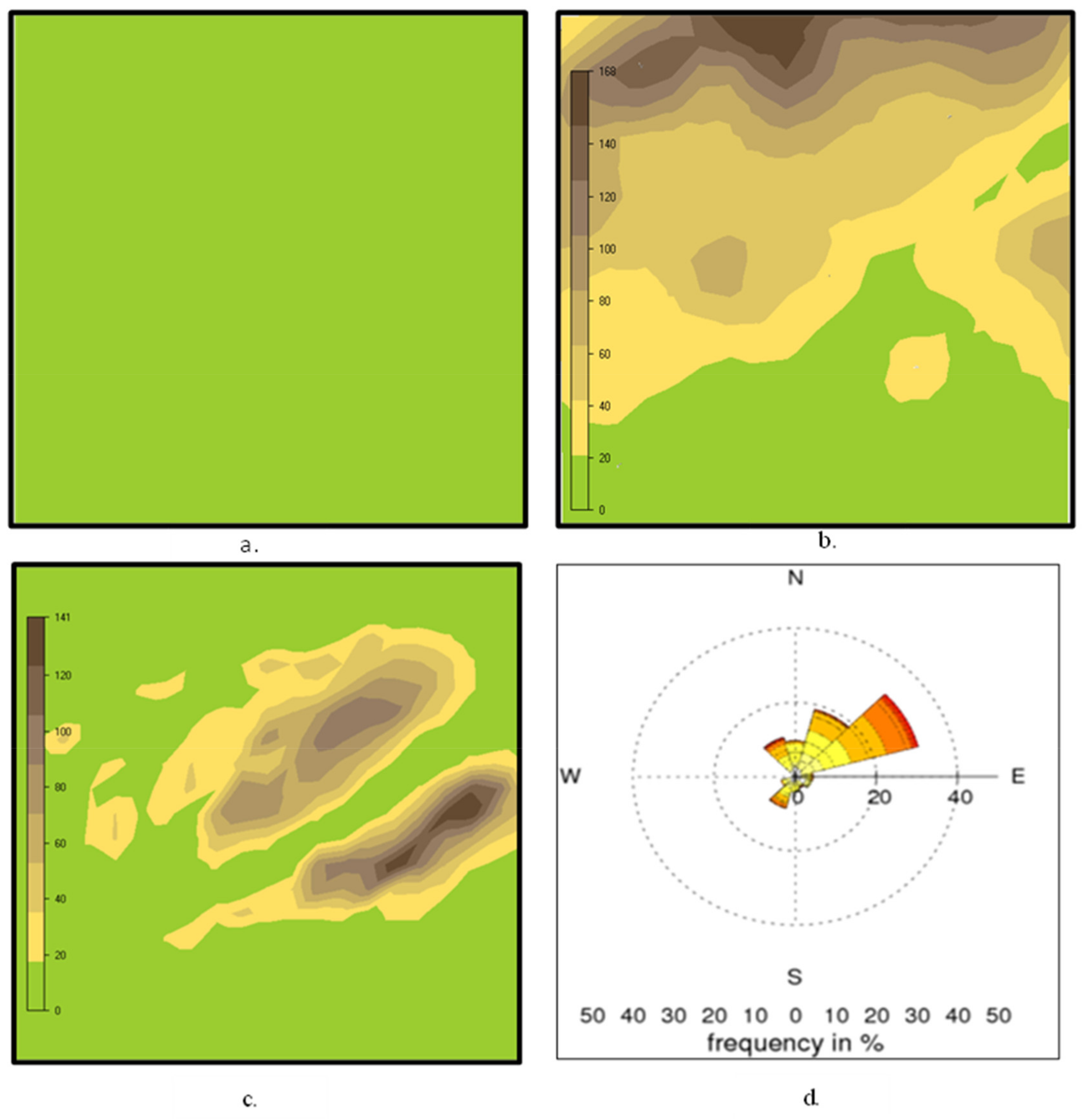
3.1. Wind Fields
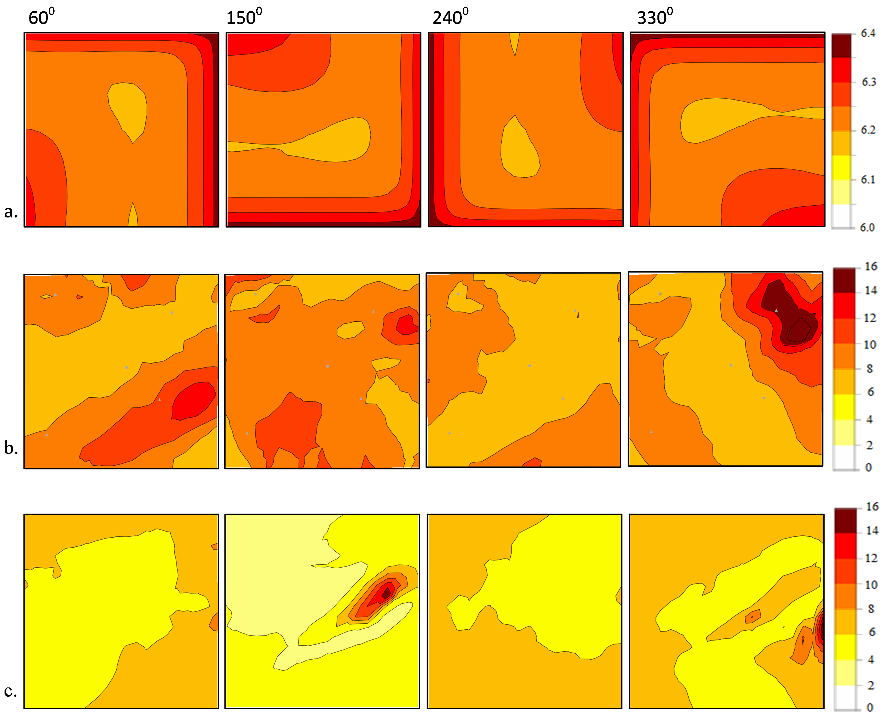
3.2. Turbulence Intensity
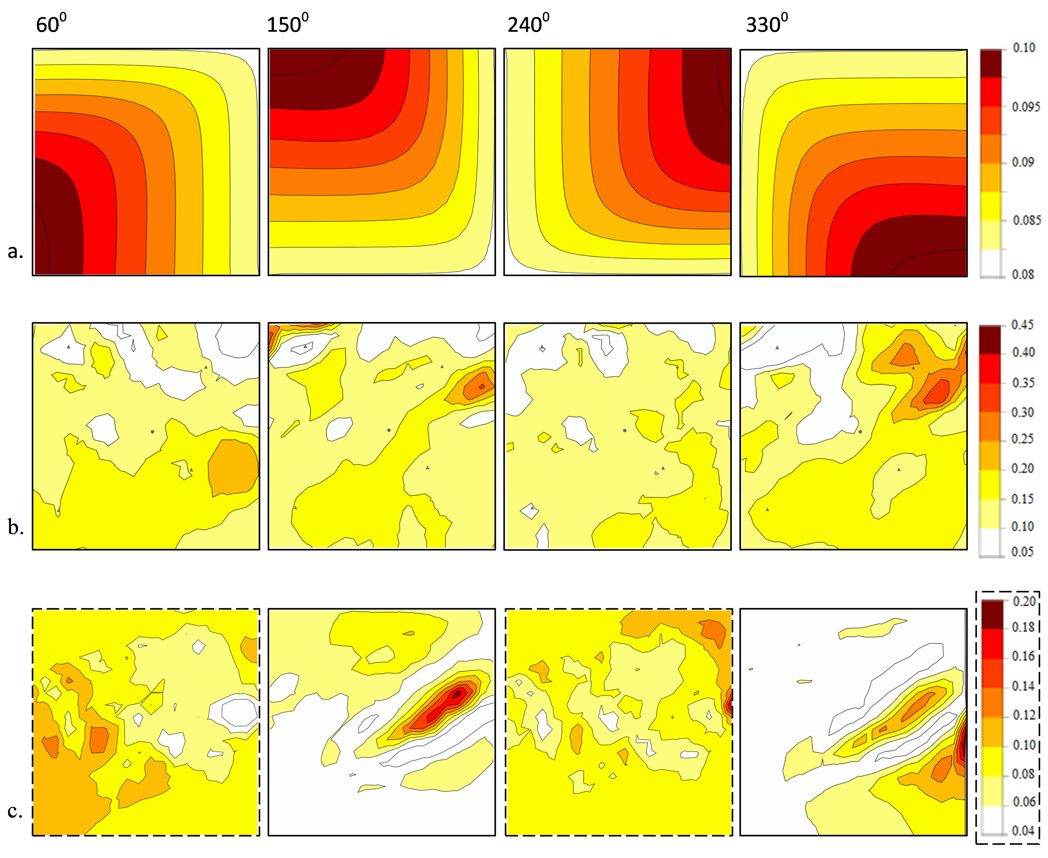
3.3. Wind Shear Exponent
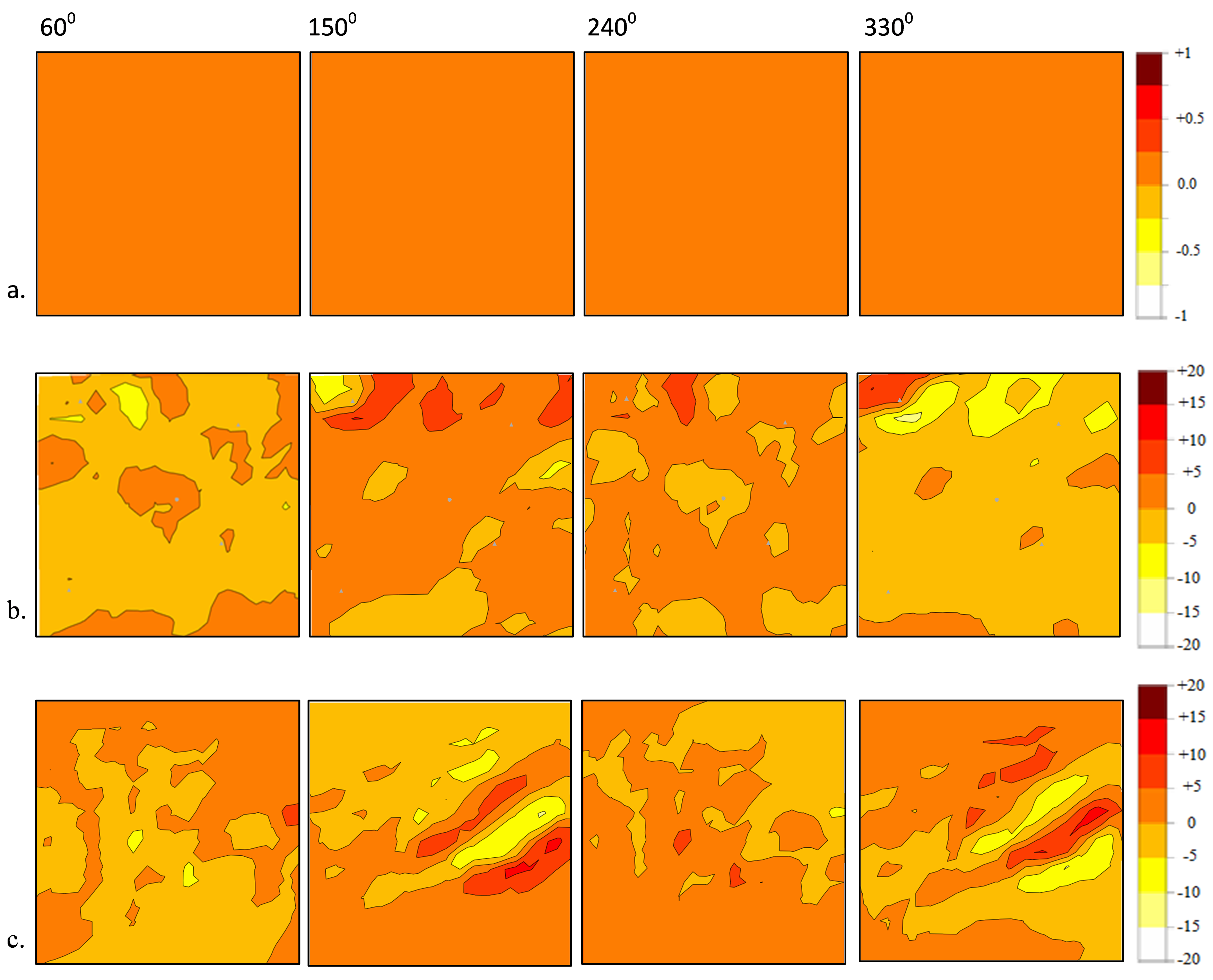
3.4. Inflow Angle
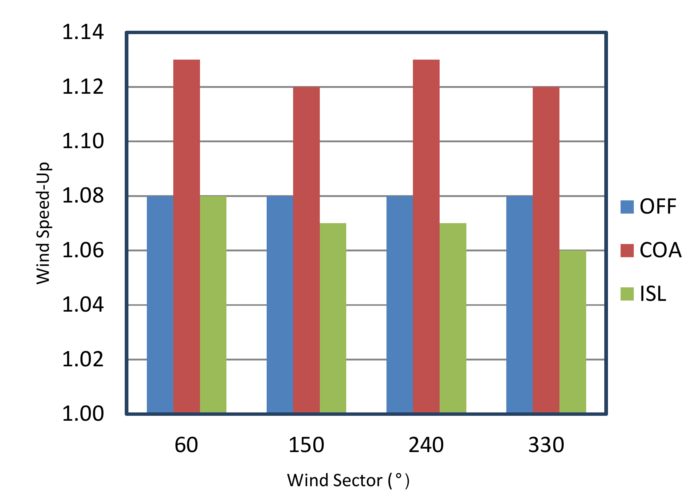
3.5. Wind Speed-Up
4. Conclusions
Author Contributions
Acknowledgments
Conflicts of Interest
References
- Kusiak, A. Share data on wind energy: Giving researchers access to information on turbine performance would allow wind farms to be optimized through data mining. Nature 2016, 529, 19–22. [Google Scholar] [CrossRef] [PubMed]
- Emeis, S. Current issues in wind energy meteorology. Meteorol. Appl. 2014, 21, 803–819. [Google Scholar] [CrossRef]
- Cetinay, H.; Kuipers, F.A.; Guven, A.N. Optimal siting and sizing of wind farms. Renew. Energy 2017, 101, 51–58. [Google Scholar] [CrossRef]
- Gao, X.; Yang, H.; Lu, L. Study on offshore wind power potential and wind farm optimization in Hong Kong. Appl. Energy 2014, 130, 519–531. [Google Scholar] [CrossRef]
- Yu, L.; Zhong, S.; Bian, X.; Heilman, W.E. Climatology and trend of wind power resources in China and its surrounding regions: A revisit using Climate Forecast System Reanalysis data. Int. J. Climatol. 2016, 36, 2173–2188. [Google Scholar] [CrossRef]
- Wang, Y.; Liu, Y.; Li, L.; Infield, D.; Han, S. Short-Term Wind Power Forecasting Based on Clustering Pre-Calculated CFD Method. Energies 2018, 11, 854. [Google Scholar] [CrossRef]
- Konopka, J.; Lopes, A.; Matzarakis, A. An Original Approach Combining CFD, Linearized Models, and Deformation of Trees for Urban Wind Power Assessment. Sustainability 2018, 10, 1915. [Google Scholar] [CrossRef]
- Di Sabatino, S.; Buccolieri, R.; Salizzoni, P. Recent advancements in numerical modelling of flow and dispersion in urban areas: A short review. Int. J. Environ. Pollut. 2013, 7, 172–191. [Google Scholar] [CrossRef]
- Blocken, B. 50 years of computational wind engineering: Past, present and future. J. Wind Eng. Ind. Aerodyn. 2014, 129, 69–102. [Google Scholar] [CrossRef]
- Yan, S.; Shi, S.; Chen, X.; Wang, X.; Mao, L.; Liu, X. Numerical simulations of flow interactions between steep hill terrain and large scale wind turbine. Energy 2018, 151, 740–747. [Google Scholar] [CrossRef]
- Toparlar, Y.; Blocken, B.; Vos, P.; Van Heijst, G.J.F.; Janssen, W.D.; van Hooff, T.; Montazeri, H.; Timmermans, H.J.P. CFD simulation and validation of urban microclimate: A case study for Bergpolder Zuid, Rotterdam. Build. Environ. 2015, 83, 79–90. [Google Scholar] [CrossRef]
- Sanderse, B.; Pijl, S.P.; Koren, B. Review of computational fluid dynamics for wind turbine wake aerodynamics. Wind Energy 2011, 14, 799–819. [Google Scholar] [CrossRef]
- Shakoor, R.; Hassan, M.Y.; Raheem, A.; Wu, Y.K. Wake effect modeling: A review of wind farm layout optimization using Jensen’s model. Renew. Sustain. Energy Rev. 2016, 58, 1048–1059. [Google Scholar] [CrossRef]
- Hansen, K.S.; Barthelmie, R.J.; Jensen, L.E.; Sommer, A. The impact of turbulence intensity and atmospheric stability on power deficits due to wind turbine wakes at Horns Rev wind farm. Wind Energy 2012, 15, 183–196. [Google Scholar] [CrossRef]
- Giahi, M.H.; Dehkordi, A.J. Investigating the influence of dimensional scaling on aerodynamic characteristics of wind turbine using CFD simulation. Renew. Energy 2016, 97, 162–168. [Google Scholar] [CrossRef]
- Cai, X.; Gu, R.; Pan, P.; Zhu, J. Unsteady aerodynamics simulation of a full-scale horizontal axis wind turbine using CFD methodology. Energy Convers. Manag. 2016, 112, 146–156. [Google Scholar] [CrossRef]
- Alaimo, A.; Esposito, A.; Messineo, A.; Orlando, C.; Tumino, D. 3D CFD analysis of a vertical axis wind turbine. Energies 2015, 8, 3013–3033. [Google Scholar] [CrossRef]
- Zanon, A.; De Gennaro, M.; Kühnelt, H. Wind energy harnessing of the NREL 5 MW reference wind turbine in icing conditions under different operational strategies. Renew. Energy 2018, 115, 760–772. [Google Scholar] [CrossRef]
- Dhunny, A.Z.; Lollchund, M.R.; Rughooputh, S.D.D.V. Wind energy evaluation for a highly complex terrain using Computational Fluid Dynamics (CFD). Renew. Energy 2017, 101, 1–9. [Google Scholar] [CrossRef]
- Blocken, B.; van der Hout, A.; Dekker, J.; Weiler, O. CFD simulation of wind flow over natural complex terrain: Case study with validation by field measurements for Ria de Ferrol, Galicia, Spain. J. Wind Eng. Ind. Aerodyn. 2015, 147, 43–57. [Google Scholar] [CrossRef]
- Cooney, C.; Byrne, R.; Lyons, W.; O’Rourke, F. Performance characterisation of a commercial-scale wind turbine operating in an urban environment, using real data. Energy Sustain. Dev. 2017, 36, 44–54. [Google Scholar] [CrossRef]
- Long, H.; Wang, L.; Zhang, Z.; Song, Z.; Xu, J. Data-driven wind turbine power generation performance monitoring. IEEE Trans. Ind. Electron. 2015, 62, 6627–6635. [Google Scholar] [CrossRef]
- Staffell, I.; Green, R. How does wind farm performance decline with age? Renew. Energy 2014, 66, 775–786. [Google Scholar] [CrossRef]
- Abolude, A.; Zhou, W. Assessment and Performance Evaluation of a Wind Turbine Power Output. Energies 2018, 11, 1992. [Google Scholar] [CrossRef]
- Bludszuweit, H.; Domínguez-Navarro, J.A.; Llombart, A. Statistical analysis of wind power forecast error. IEEE Trans. Power Syst. 2008, 23, 983–991. [Google Scholar] [CrossRef]
- Carrillo, C.; Montaño, A.O.; Cidrás, J.; Díaz-Dorado, E. Review of power curve modelling for wind turbines. Renew. Sustain. Energy Rev. 2013, 21, 572–581. [Google Scholar] [CrossRef]
- Schlechtingen, M.; Santos, I.F.; Achiche, S. Using data-mining approaches for wind turbine power curve monitoring: A comparative study. IEEE Trans. Sustain. Energy 2013, 4, 671–679. [Google Scholar] [CrossRef]
- Shokrzadeh, S.; Jozani, M.J.; Bibeau, E. Wind turbine power curve modeling using advanced parametric and nonparametric methods. IEEE Trans. Sustain. Energy 2014, 5, 1262–1269. [Google Scholar] [CrossRef]
- Villanueva, D.; Feijóo, A. Normal-based model for true power curves of wind turbines. IEEE Trans. Sustain. Energy 2016, 7, 1005–1011. [Google Scholar] [CrossRef]
- Whale, J.; McHenry, M.P.; Malla, A. Scheduling and conducting power performance testing of a small wind turbine. Renew. Energy 2013, 55, 55–61. [Google Scholar] [CrossRef]
- Li, S.; Wunsch, D.C.; O’Hair, E.A.; Giesselmann, M.G. Using neural networks to estimate wind turbine power generation. IEEE Trans. Energy Convers. 2001, 16, 276–282. [Google Scholar]
- Lydia, M.; Kumar, S.S.; Selvakumar, A.I.; Kumar, G.E.P. A comprehensive review on wind turbine power curve modeling techniques. Renew. Sustain. Energy Rev. 2014, 30, 452–460. [Google Scholar] [CrossRef]
- Jafarian, M.; Ranjbar, A.M. Fuzzy modeling techniques and artificial neural networks to estimate annual energy output of a wind turbine. Renew. Energy 2010, 35, 2008–2014. [Google Scholar] [CrossRef]
- Zamani, M.H.; Riahy, G.H.; Ardakani, A.J. Modifying power curve of variable speed wind turbines by performance evaluation of pitch-angle and rotor speed controllers. In Proceedings of the 2007 IEEE Canada Electrical Power Conference, Montreal, QC, Canada, 25–26 October 2007; pp. 347–352. [Google Scholar]
- Tindal, A.; Johnson, C.; LeBlanc, M.; Harman, K.; Rareshide, E.; Graves, A. Site-specific adjustments to wind turbine power curves. In Proceedings of the AWEA Wind Power Conference, Houston, TX, USA, 4 June 2008. [Google Scholar]
- Lubitz, W.D. Impact of ambient turbulence on performance of a small wind turbine. Renew. Energy 2014, 61, 69–73. [Google Scholar] [CrossRef]
- Uchida, T. LES Investigation of Terrain-Induced Turbulence in Complex Terrain and Economic Effects of Wind Turbine Control. Energies 2018, 11, 1530. [Google Scholar] [CrossRef]
- Bilal, M.; Birkelund, Y.; Homola, M.; Virk, M.S. Wind over complex terrain–Microscale modelling with two types of mesoscale winds at Nygårdsfjell. Renew. Energy 2016, 99, 647–653. [Google Scholar] [CrossRef]
- Dhunny, A.Z.; Lollchund, M.R.; Rughooputh, S.D.D.V. Numerical analysis of wind flow patterns over complex hilly terrains: Comparison between two commonly used CFD software. Int. J. Glob. Energy Issues 2016, 39, 181–203. [Google Scholar] [CrossRef]
- Ferziger, J.H.; Peric, M. Computational Methods for Fluid Mechanics; Springer: Berlin, Germany, 2002. [Google Scholar]
- Bechmann, A.; Sørensen, N.N.; Berg, J.; Mann, J.; Réthoré, P.E. The Bolund experiment, part II: Blind comparison of microscale flow models. Bound.-Lay. Meteorol. 2011, 141, 245. [Google Scholar] [CrossRef]
- WindSim WindSim Manual Sourced. Available online: https://www.windsim.com/products/windsim-brochures.aspx (accessed on 24 December 2017).
- Ray, M.L.; Rogers, A.L.; McGowan, J.G. Analysis of Wind Shear Models and Trends in Different Terrains; Renewable Energy Research Laboratory, Department of Mechanical & Industrial Engineering, University of Massachusetts: Amherst, MA, USA, 2006. [Google Scholar]
- Türk, M.; Emeis, S. The dependence of offshore turbulence intensity on wind speed. J. Wind Eng. Ind. Aerodyn. 2010, 98, 466–471. [Google Scholar] [CrossRef]
- Newman, J.F.; Klein, P.M. The impacts of atmospheric stability on the accuracy of wind speed extrapolation methods. Resources 2014, 3, 81–105. [Google Scholar] [CrossRef]
- Drew, D.R.; Barlow, J.F.; Lane, S.E. Observations of wind speed profiles over Greater London, UK, using a Doppler lidar. J. Wind Eng. Ind. Aerodyn. 2013, 121, 98–105. [Google Scholar] [CrossRef]
- Shu, Z.R.; Li, Q.S.; He, Y.C.; Chan, P.W. Observations of offshore wind characteristics by Doppler-LiDAR for wind energy applications. Appl. Energy 2016, 169, 150–163. [Google Scholar] [CrossRef]
- Farrugia, R.N. The wind shear exponent in a Mediterranean island climate. Renew. Energy 2003, 28, 647–653. [Google Scholar] [CrossRef]
- Blackadar, A.K. Turbulence and Diffusion in the Atmosphere; Springer: Berlin, Germany, 1997. [Google Scholar]
- Emeis, S. Wind Energy Meteorology; Springer: Berlin, Germany, 2013. [Google Scholar]


| Terrain/Sector | 60° | 150° | 240° | 330° |
|---|---|---|---|---|
| OFF WTPC | 21% | 21% | 21% | 21% |
| COA WTPC | 30% | 22% | 30% | 22% |
| ISL WTPC | 21% | 19% | 19% | 17% |
© 2018 by the authors. Licensee MDPI, Basel, Switzerland. This article is an open access article distributed under the terms and conditions of the Creative Commons Attribution (CC BY) license (http://creativecommons.org/licenses/by/4.0/).
Share and Cite
Abolude, A.T.; Zhou, W. A Comparative Computational Fluid Dynamic Study on the Effects of Terrain Type on Hub-Height Wind Aerodynamic Properties. Energies 2019, 12, 83. https://doi.org/10.3390/en12010083
Abolude AT, Zhou W. A Comparative Computational Fluid Dynamic Study on the Effects of Terrain Type on Hub-Height Wind Aerodynamic Properties. Energies. 2019; 12(1):83. https://doi.org/10.3390/en12010083
Chicago/Turabian StyleAbolude, Akintayo T., and Wen Zhou. 2019. "A Comparative Computational Fluid Dynamic Study on the Effects of Terrain Type on Hub-Height Wind Aerodynamic Properties" Energies 12, no. 1: 83. https://doi.org/10.3390/en12010083
APA StyleAbolude, A. T., & Zhou, W. (2019). A Comparative Computational Fluid Dynamic Study on the Effects of Terrain Type on Hub-Height Wind Aerodynamic Properties. Energies, 12(1), 83. https://doi.org/10.3390/en12010083