Article

Analysis of the Performance of Various PV Module Technologies in Peru

1
IDEA Research Group, University of Jaén, Campus de Las Lagunillas, 23071 Jaén, Spain
2
Renewable Energy Center, National Engineering University, Av. Túpac Amaru 210, Of. B1-260, Lima 25, Peru
*
Author to whom correspondence should be addressed.
Energies 2019, 12(1), 186; https://doi.org/10.3390/en12010186
Submission received: 13 December 2018 / Revised: 2 January 2019 / Accepted: 2 January 2019 / Published: 8 January 2019

Abstract

:
A knowledge gap exists about the actual behavior of PV grid-connected systems (PVGCS) using various PV technologies in Peru. This paper presents the results of an over three-year-long performance evaluation of a 3.3-kWp monocrystalline silicon (sc-Si) PVGCS located in Arequipa, a 3.3-kWp sc-Si PVGCS located in Tacna, and a 3-kWp policrystalline (mc-Si) PVGCS located in Lima. An assessment of the performance of a 3.5-kWp amorphous silicon/crystalline silicon hetero-junction (a-Si/µc-Si) PVGCS during over one and a half years of being in Lima is also presented. The annual final yields obtained lie within 1770–1992 kWh/kW, 1505–1540 kWh/kW, and 736–833 kWh/kW for Arequipa, Tacna, and Lima, respectively, while the annual PV array energy yield achieved by a-Si/µc-Si is 1338 kWh/kW. The annual performance ratio stays in the vicinity of 0.83 for sc-Si in Arequipa and Tacna while this parameter ranges from 0.70 to 0.77 for mc-Si in Lima. An outstanding DC annual performance ratio of 0.97 is found for a-Si/µc-Si in the latter site. The use of sc-Si and presumably, mc-Si PV modules in desert climates, such as that of Arequipa and Tacna, is encouraged. However, sc-Si and presumably, mc-Si-technologies experience remarkable temperature and low irradiance losses in Lima. By contrast, a-Si/µc-Si PV modules perform much better in the latter site thanks to being less influenced by both temperature and low light levels.

1. Introduction

The cumulative photovoltaic (PV) power on the planet at the end of 2017 was around 415 GW while the compound annual growth rate of PV installations reached 24% during the period of 2010–2017 [1]. According to some estimates, global PV demand in 2018 will likely fall to some 85 GW down from the 104 GW expected, mainly due to the contraction of the Chinese market [2] which in turn will result in falling PV module prices. Consequently, some other markets—Europe, USA, India, Japan, and Latin America, among others—will benefit from this situation in the short term. Anyway, PV will turn into a major source of clean energy within the next few years since PV systems have proven durable, reliable, and cost-competitive.
It is a well-known fact that PV system outdoor behavior depends on the solar resource in conjunction with a suitable PV technology, quality of balance-of-system components, and proper designs. Indeed, PV performance is influenced by a wide variety of site-related environmental parameters, such as temperature, spectral effects, angular losses, partial shading, low irradiance levels, and soiling losses. PV performance has already been widely addressed for sites located in countries with temperate climates [3,4,5,6,7,8,9,10,11,12,13,14].
Nevertheless, few reports can be found for sites with desert climates, and even far fewer for sites with such climates in countries with emerging economies. In addition to the relative scarcity of such studies, they turn out to be difficult to compare with each other. Thus, in some cases, in-plane irradiance is measured by using a co-planar calibrated crystalline silicon (c-Si) solar cell or PV module as a PV reference device (PVRD) while thermopile-based or photodiode-based pyranometers are used in other studies. Moreover, PV modules are left unclean during the period under investigation in some cases while in others, they are regularly or sporadically cleaned. Unfortunately, some of these contributions do not even mention whether any cleaning pattern has been followed or not.
A study carried out in Sohar (Oman) by Kazem et al. [15] reported an annual performance ratio of 0.85 and an annual final yield of 1875 kWh·kW−1 for a 1.4-kW policrystalline (mc-Si) PV grid-connected system (PVGCS) with modules left unclean. Eke and Demircan [16] analyzed the behavior of a 2.73-kW monocrystalline (sc-Si) PVGCS with modules also left unclean in Mugla (Turkey)—a site with a dry climate—thus, finding an annual performance ratio and an annual final yield of 0.72 and 1414 kWh·kW−1, respectively. The results of the analysis of a 5.52-kW mc-Si PVGCS with modules cleaned on a weekly basis in an arid location, such as Kerman (Iran)—annual performance ratio and annual final yield of 0.83 and 1964 kWh·kW−1, respectively—were presented by Edalati et al. [17]. Two copper indium gallium selenide (CIGS) PVGCS (<100 kW) with modules left unclean during three months located in Azda and Sawda (Kuwait) had an average annual generation of 1643 kWh·kW−1 [18], while monthly values of the performance ratio were within the ranges 0.70–0.82 (Azda) and 0.70–0.85 (Sawda).
Unfortunately, literature on quantifying the PV performance in Latin American sites with arid or semi-arid climates is very rare and limited to Chile. Some values of the annual final yield calculated for PV modules sporadically cleaned in Antofagasta (Chile) have been reported [19]: 1760 kWh·kW−1 and 1690 kWh·kW−1 were found for sc-Si and amorphous silicon/crystalline silicon heterojunction (a-Si/µc-Si) PVGCS, respectively, while values computed of annual performance ratios were equal to 0.79 for the former and 0.78 for the latter. Likewise, the annual output of three PV systems monitored during two years in Santiago (Chile) with weekly cleaning routines reached 1459–1444 kWh·kW−1 for sc-Si, 1419–1373 kWh·kW−1 for mc-Si, and 1248–1236 for a-Si/µc-Si [20]. Annually averaged values of performance ratios over the course of the two-year experimental campaign carried out in these three systems were also calculated: 0.77–0.76 (sc-Si), 0.76–0.75 (mc-Si), and 0.76–0.73 (a-Si/µc-Si).
Peru is situated in western South America between 0° and 10° S latitude and between 70° and 81° W longitude, approximately. The world map of the Köppen–Geiger climate classification [21] describes the wide variety of existing climates in this country: Tropical monsoon (Am), cold semi-arid (BSk), cold desert (BWk), hot semi-arid (Bsh), hot desert (BWh), oceanic (Cfb), tropical rainforest (Af), tropical savanna climate (Aw), and subtropical highland variety (CWb).
Peru has experienced a remarkable development during the last years with an annual average increase of the gross domestic product (GDP) of 3.1% between 2014 and 2017 [22]. This economic growth is heavily reliant on fossil fuels, as oil and natural gas combined accounted for 85% of the total primary energy supply in 2016 [23]. On the down side, the detrimental impact on the environment of this fossil-based development has already been studied [24]. Despite having a marginal share of Peru’s electricity mix at present, PV has a great potential in this country since large areas around the coast with desert and semi-arid climates are blessed with an outstanding solar resource. In this respect, it is worth noting that several PV plants already operate in Peru. Just to give some instances, two 20-MW a-Si PV plants were commissioned in 2012: One in Majes and the other in La Joya. Likewise, two 20-MW mc-Si PV plants have operated since then in Tacna and Moquegua, respectively. More recently, the largest PV plant of Peru was commissioned in 2018 with 144.8 MW of mc-Si PV modules installed in Moquegua [25,26,27]. Unfortunately, many of the lessons learned and the detailed operation results of such large PV systems are not publicly available. This fact may be understandable to some extent as these PV plants are operated and maintained by private companies. Nevertheless, PV developers and academicians cannot have access to this information that would highly improve their designs and lead to a better understanding of the behavior of this technology in Peru. In fact, there is still a lack of available analyses regarding how PV materials perform under Peruvian outdoor conditions. This is a crucial issue, as a bad choice of a PV technology for a specific location may result in a faulty design of a PV project [28].
In view of the considerations above, this paper is aimed at trying to fill the gap in knowledge on the performance of various PV materials in Peruvian sites with different climatic conditions. To this end, two 3.3-kWp PVGCS using sc-Si PV modules were installed in Arequipa and Tacna and then investigated over more than three years. A 3-kWp PVGCS using mc-Si PV modules was installed in Lima and then analyzed during a similar time period. Last, a 3.5-kWp PVGCS using a-Si/µc-Si PV modules was installed in the latter site to be studied over more than one and a half years. The experimental campaign conducted did not have a special originality. Indeed, it was based on the study of data related to the performance of four PV systems located in Peru, which were monitored over a meaningful time period. However, this is precisely where the novelty of this work lies, as no results of the analysis of the behavior of different PV technologies in this Andean country were publicly available at the time of this writing.
This paper is organized into four sections. Following this introduction, Section 2 describes the experimental setup used and provides definitions of the parameters and performance metrics calculated—together with their mathematical expressions—of the PVGCS under scrutiny. Section 3 presents and discusses the results of the yields and performance metrics over the course of the experimental campaign conducted for the PVGCS analyzed. These results are compared with those gleaned from other studies internationally. Finally, the conclusions presented in Section 4 put an end to this work.

2. Materials and Methods

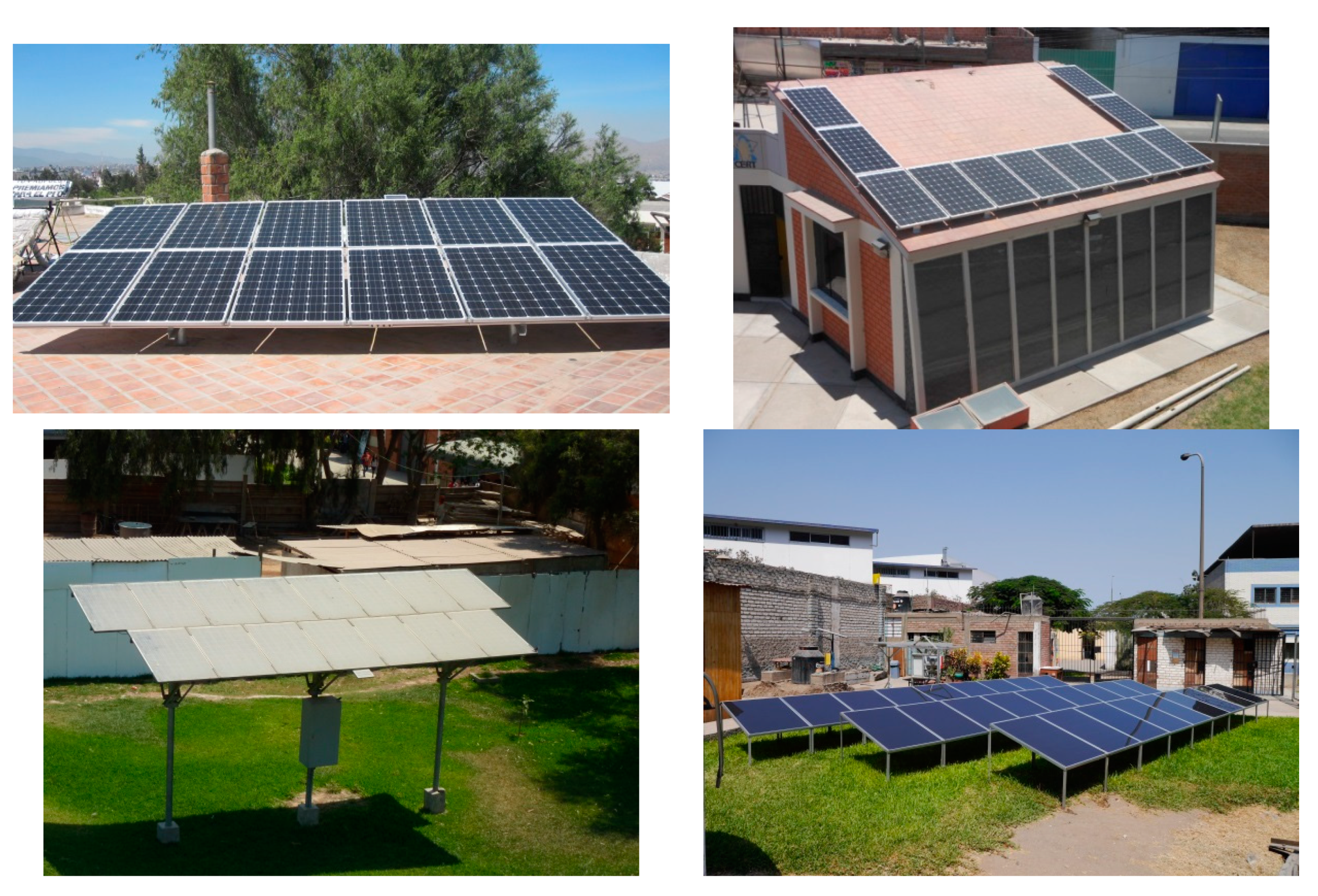
2.1. Experimental Setup

Four PVGCS using different PV materials were installed in three locations in Peru. PVGCS #1 was installed at the National University of San Agustín in Arequipa (latitude 16.40° S, longitude 71.53° W, elev. 2335 m). PVGCS #2 is located at the National University of Jorge Basadre Grohmann in Tacna (latitude 18.02° S, longitude 70.25° W, elev. 562 m). PVGCS #3 and PVGCS #4 are located at the National University of Engineering in Lima (latitude 12.02° S, longitude 77.05° W, elev. 161 m) and are some 1 km away from each other. The world map of the Köppen–Geiger climate classification [21] describes the climatic conditions of the three sites. Thus, the climate in Arequipa is borderline between cold desert climate (BwK) and hot desert climate (Bwh), while those of Lima and Tacna are both classified Bwh. In this sense, Table 1 provides some quantitative climate information of the sites under investigation. The four PV systems that have provided the experimental data to this work are shortly described below.
PVGCS #1 and PVGCS #2 are 3.3-kWp twin installations, which were commissioned in June 2015 and May 2015, respectively. Both installations have a PV field comprised by 12 series-connected sc-Si PV modules 275-Wp rated each. Each PV field is connected to a 3010-W rated Steca Coolcept-x 3010x inverter. PVGCS #3 was commissioned in April 2015 and its PV field is composed by 14 series-connected mc-Si PV modules 215-Wp rated each, totaling 3010 Wp. This PV field is connected to a 3000-W rated Steca 3000 inverter. PVGCS #4 was commissioned in July 2016 and was built using a two-input multi-string 3000-W rated Sunny Boy 3000TL inverter to which a field composed by three strings of 9 series-connected a-Si/µc-Si PV modules each rated 128-Wp was connected. The PV subfield connected to one of the inverter inputs is comprised by two such strings connected in parallel, totaling 2304 Wp. The other inverter input is connected to the remaining string totaling 1152 Wp. The latter string has not been under investigation here, as detailed hereafter.
All the PV fields described in the preceding paragraph are equator-facing with a tilt angle of 15°. Note that the inverter sizing factor—ratio of rated inverter output power to PV field power at STC [32,33]—used in the design of the systems above ranges from 0.87 (Lima, a-Si/µc-Si) to 1 (Lima, mc-Si) through 0.91 (Arequipa and Tacna, sc-Si). Moreover, the nameplate rating of the PV modules was used in every calculation. The characteristics of each PV field are gathered in Table 2. Figure 1 shows photographs of all the PV systems under scrutiny in this paper.
The monitoring systems used in each PVGCS are based on quality marketed components (Carlo Gavazzi’s brand) and are controlled by ‘OLE for Process Control’ technology, a communication standard based on Microsoft technology, in combination with LabVIEWTM software. Each monitoring system registers the following parameters: Output AC (alternating current) voltage, output AC current, output apparent, reactive and real output AC power (Pout, in W), frequency, power factor, cumulative output AC energy, input DC (direct current) voltage, input DC current, input DC power (PA, in W), in-plane irradiance (Gi, in W·m−2), module temperature (Tmod, in °C), and ambient temperature (Tamb, in °C). Data were taken at 15-s intervals.
Pt100 resistive thermal detectors (RTD) glued on the rear surface of the PV modules were used to measure their temperature, while a thermocouple with radiation shield was also used to measure Tamb. In every system, the in-plane irradiance was measured by using a co-planar calibrated sc-Si solar cell as a PV reference device (PVRD). Neither the PV fields nor the PVRD corresponding to PVGCS #1–#3 were cleaned over the course of the experimental campaign, but special care was taken to remove solid substances, such as bird droppings, on a weekly basis. As the spectral responses of the PVRD used in the latter systems very closely match the spectral responses of their PV fields, such sensors measure the PV-usable portion of the in-plane broadband irradiation. It follows that the values recorded of Gi correspond to the effective irradiance to which the PV fields of PVGCS #1–#3 are sensitive. As PVRD were kept in the same level of soiling as PV modules, the short circuit current of such sensors incorporated the influence of varying spectral irradiance, angle-of-incidence losses as well as the soiling impact. In this sense, as PV developers and operators are mainly concerned with the power delivered by the PV field, the best and easiest way to measure the effective in-plane irradiance is with a co-planar calibrated PVRD with, ideally, the same spectral response as the PV field [34].
Unlike PVGCS #1–#3, both the 2304-Wp PV field connected to one of the inputs of the inverter of PVCGS #4 and its co-planar calibrated sc-Si solar cell were cleaned weekly. Ideally, effective irradiance measurements would require a PVRD of the same technology and state of cleanliness as the a-Si/µc-Si PV field. However, stability issues of thin film PVRD motivated the decision to use a calibrated sc-Si solar cell, at the cost of increasing uncertainty. True, broadband irradiation measurements combined with equations that capture the impact of the spectrum and angular losses may be used to compute the effective irradiance. However, a thermopile pyranometer—not available in the experimental setup—is required for this complex approach, which may also lead to noticeable uncertainties related to the results obtained [35,36,37]. In this sense, it is worth noting that other authors have adhered to the practice of using c-Si PVRD to measure the portion of irradiance used by thin film PV materials [19,38,39,40].

2.2. Calculated Parameters and Performance Metrics

Time series of yields and performance metrics were calculated for the four PVGCS under study, as recommended in the IEC 61724:2017-1 standard [34].
The monthly in-plane irradiation (Hi, in Wh·m−2) can be obtained as follows:
H i = k m G i , k · τ k
where Gi,k (W·m−2) is the k-th recorded value of the in-plane irradiance, m is the number of instances recorded during a month, and τk (h) is the duration of the k-th recording interval. Measurements were taken every 15 s, τk = 1/240 h.
The monthly DC energy (EA, in Wh) was calculated by:
E A = k m P A , k · τ k
where PA,k (W) is the k-th recorded value of the input DC power.
The monthly PV module AC output (Eout, in Wh) was given by:
E out = k m P out , k · τ k
where Pout,k (W) is the is the k-th recorded value of the output AC power.
The monthly PV array energy yield (YA, in Wh·W−1) was equal to EA divided by the PV module rating (P0, in W):
Y A = E A P 0
The monthly final PV system yield (Yf, in Wh·W−1) was calculated as follows:
Y f = E out P 0
The monthly reference yield (Yr, in Wh·W−1) was given by:
Y r = H i G *
where G* (W·m−2) is the reference in-plane irradiance (1000 W·m−2) at which P0 was determined.
The monthly performance ratio (PR) was equal to Yf divided by Yr.
P R = Y f Y r = E out P 0 H i G *
Last, the monthly DC performance ratio (PRDC) was given by the following equation:
P R DC = E A P 0 H i G *
Annual values of final yield (Yf,annual, in Wh·W−1), PV array energy yield (YA,annual, in Wh·W−1), reference yield (Yr,annual, in Wh·W−1), performance ratio (PRannual), and DC performance ratio (PRDC,annual) were calculated using Equations (1)–(8) and enlarging the considered reporting time up to one year.

3. Results and Discussion
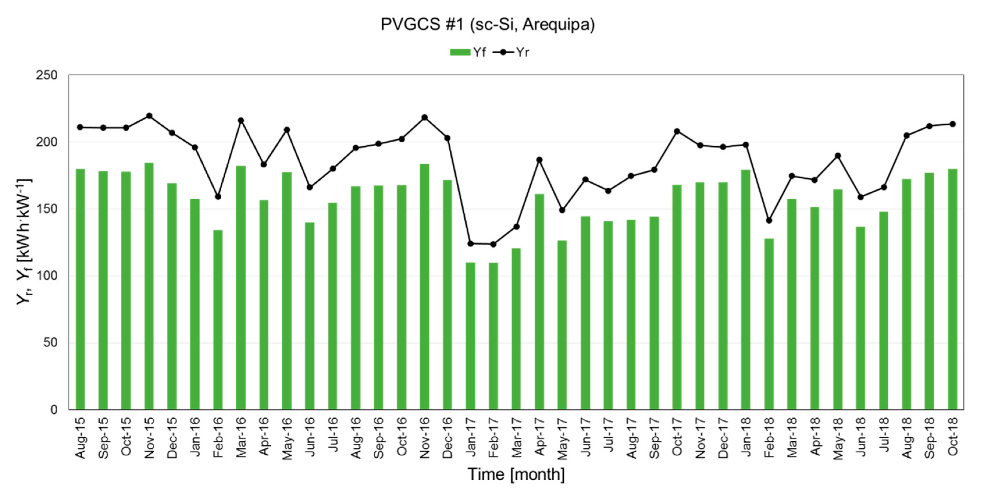
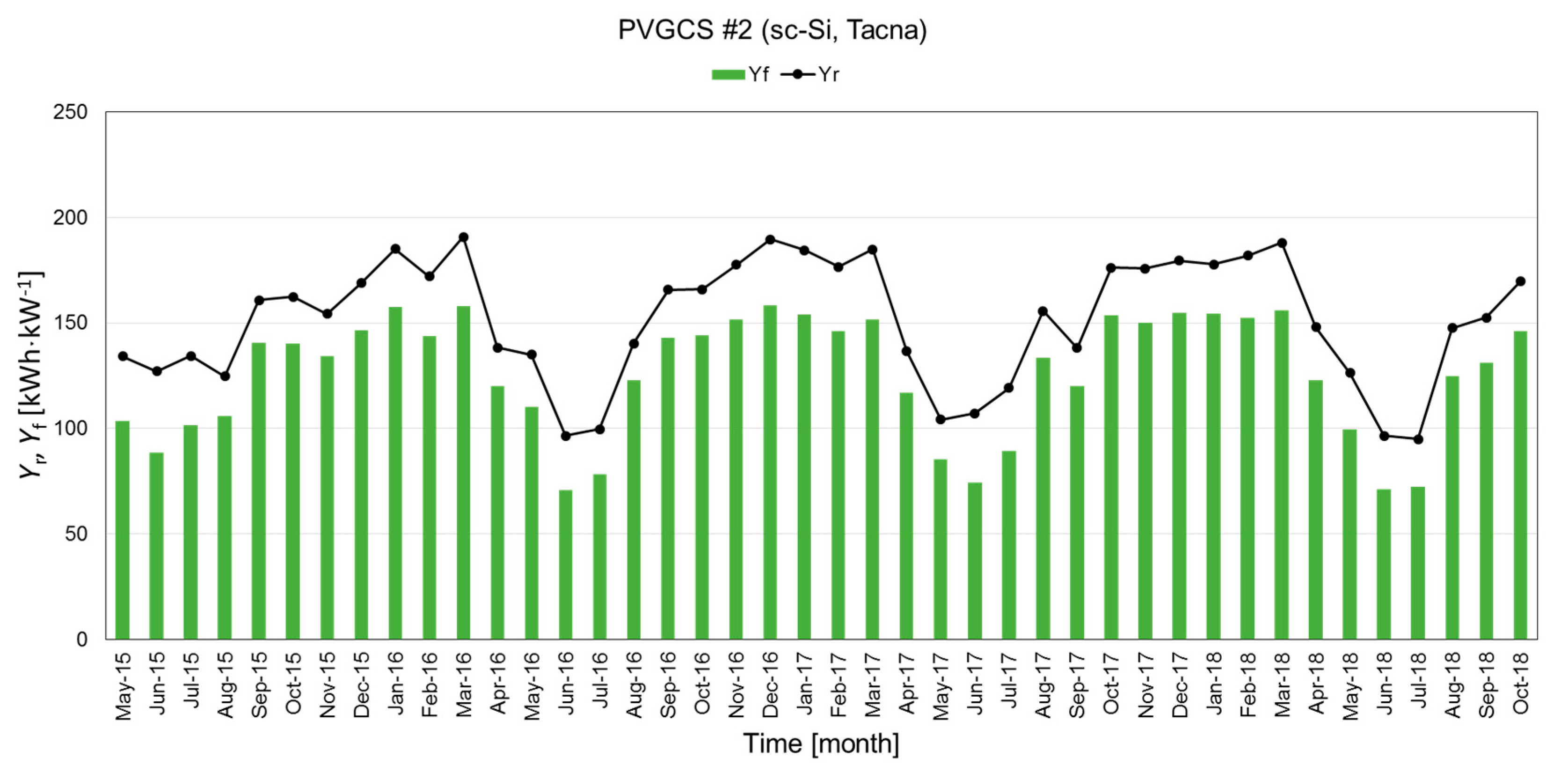
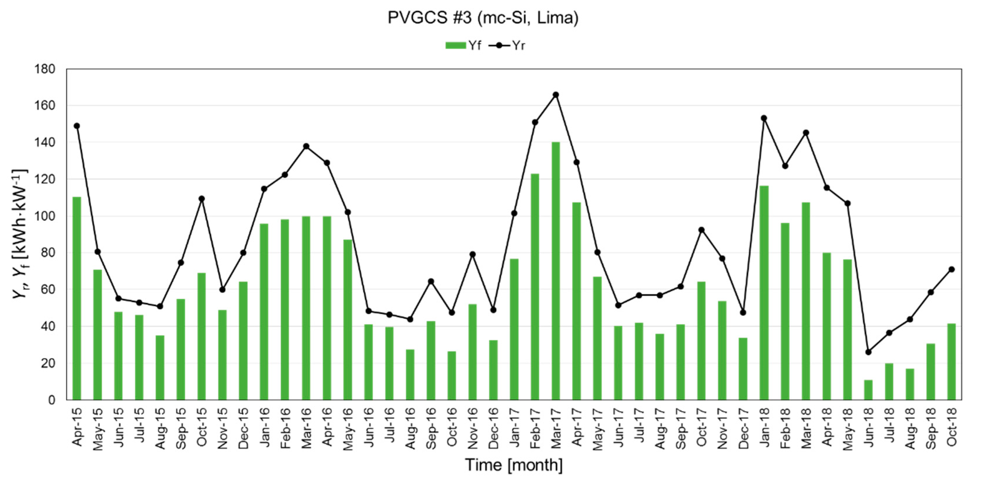
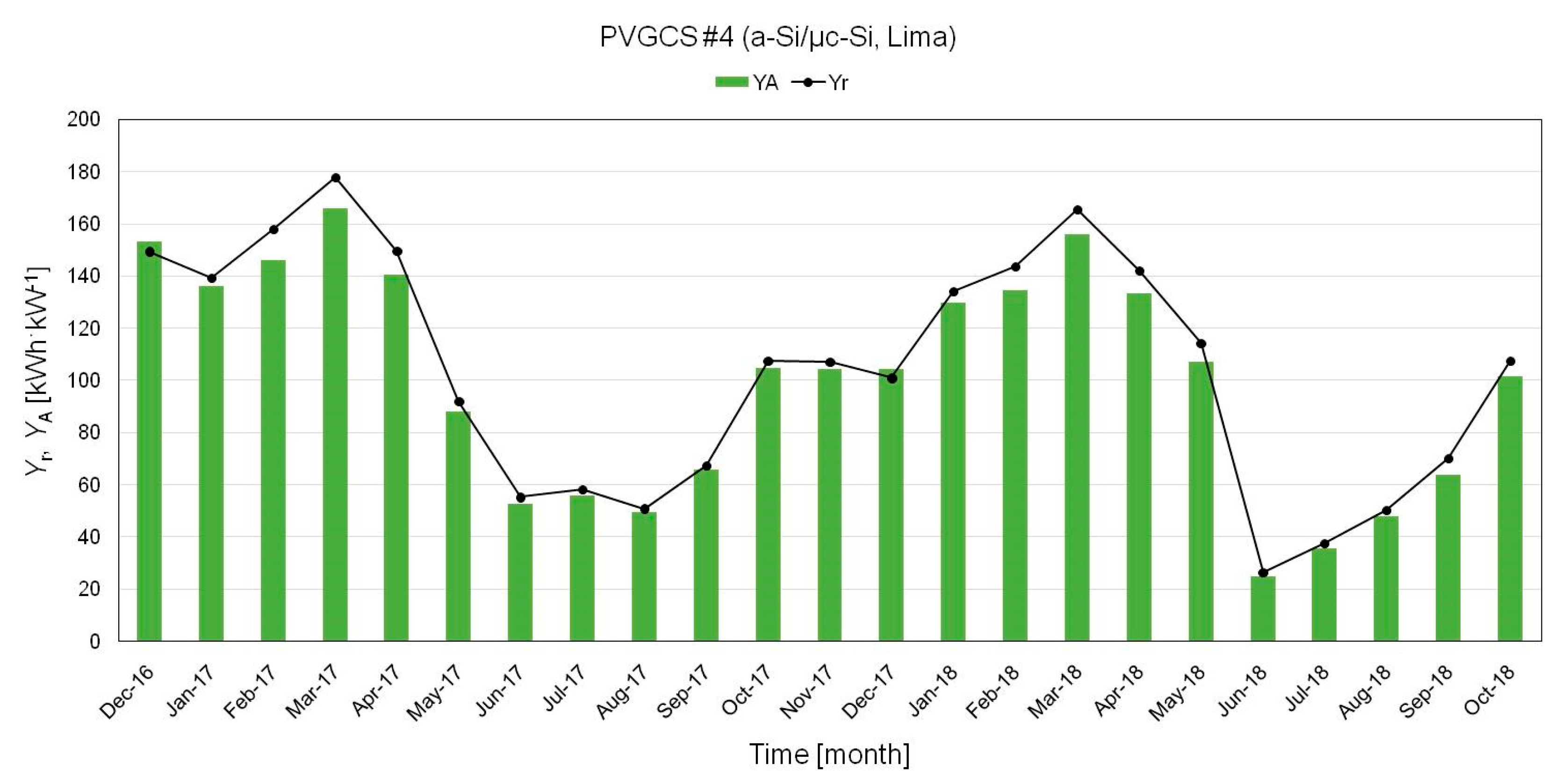
This section presents the results of the yields and performance metrics obtained during the experimental campaign. Most monitoring data corresponding to PVGCS #1 and #4 gleaned in June–July 2015 and June–November 2016, respectively, proved invalid or inconsistent. Consequently, such data are not taken into account in the periods under study, which last over three years for PVGCS #1–#3 and over one and a half year for PVGCS #4.

3.1. Monthly Yields

Figure 2, Figure 3 and Figure 4 show the values of Yr and Yf for PVGCS #1–#3 while Figure 5 depicts the values of Yr and YA for PVGCS #4. Such values are plotted over the period under study of each system. It must be remembered that values of Yr were computed using effective values of Gi, as the latter parameter was measured by means of a PVRD. Anyway, a noticeable correlation between the PV output and the solar resource exists. Consequently, the discussion that follows for Yr also holds qualitatively for Yf (YA, for PVGCS #4).
Arequipa shows the relatively most stable monthly irradiation profile, staying between 150 and 200 kWh·kW−1 for the most part of the experimental campaign. Seasonality was more pronounced in Tacna, as values of Yr were higher in December–March and lower in May–July. Specifically, the seasonal spread that this parameter experiences—the difference between its maximum and minimum value—is around 100 kWh·kW−1. It is clear that Lima has the lowest irradiation profile, resulting in far smaller monthly yields than those achieved in Arequipa and Tacna. Lima also shows the most remarkable seasonal trend of the solar resource over the period under investigation. Thus, as shown in Figure 4, Yr stays below 60 kWh·kW−1 during winter months—lowering to 30 kWh·kW−1 in June 2018—while this parameter peaks at values above 160 kWh·kW−1 in March. It should be remarked that Yf for PVGCS #3—mc-Si, left unclean—is lower than YA for PVGCS #4—a-Si/µc-Si, weekly cleaned PV subfield. Of course, both yields cannot be directly compared, as balance-of-system losses were not subtracted from YA. However, these noticeable differences between the yields of both systems located in Lima will be dealt with in-depth in the subsequent analysis regarding performance.

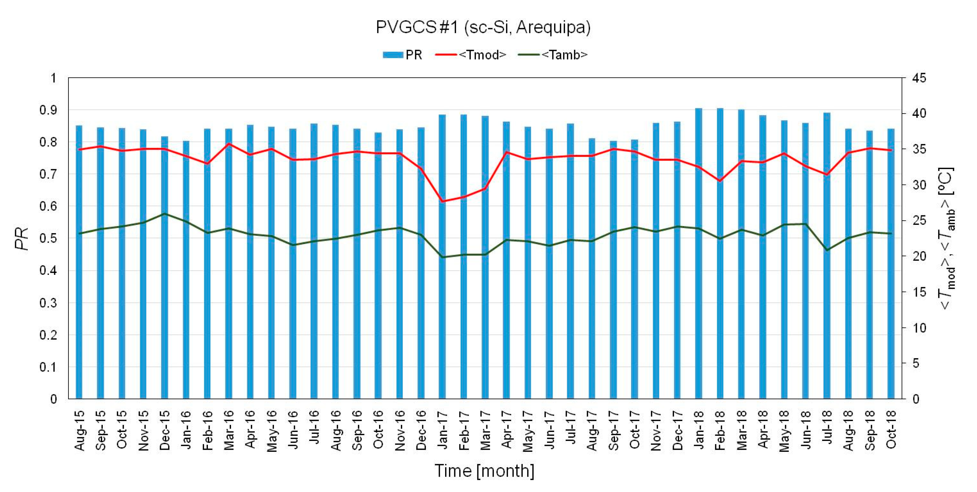
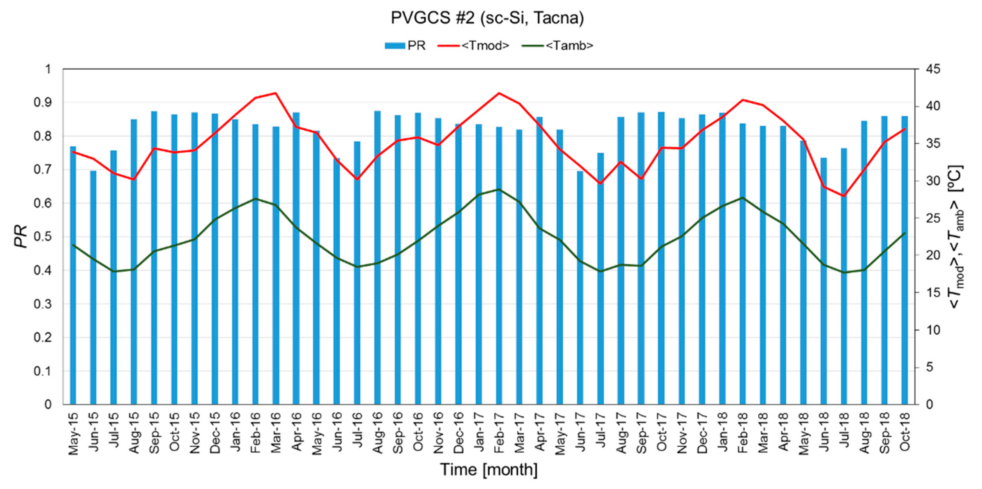
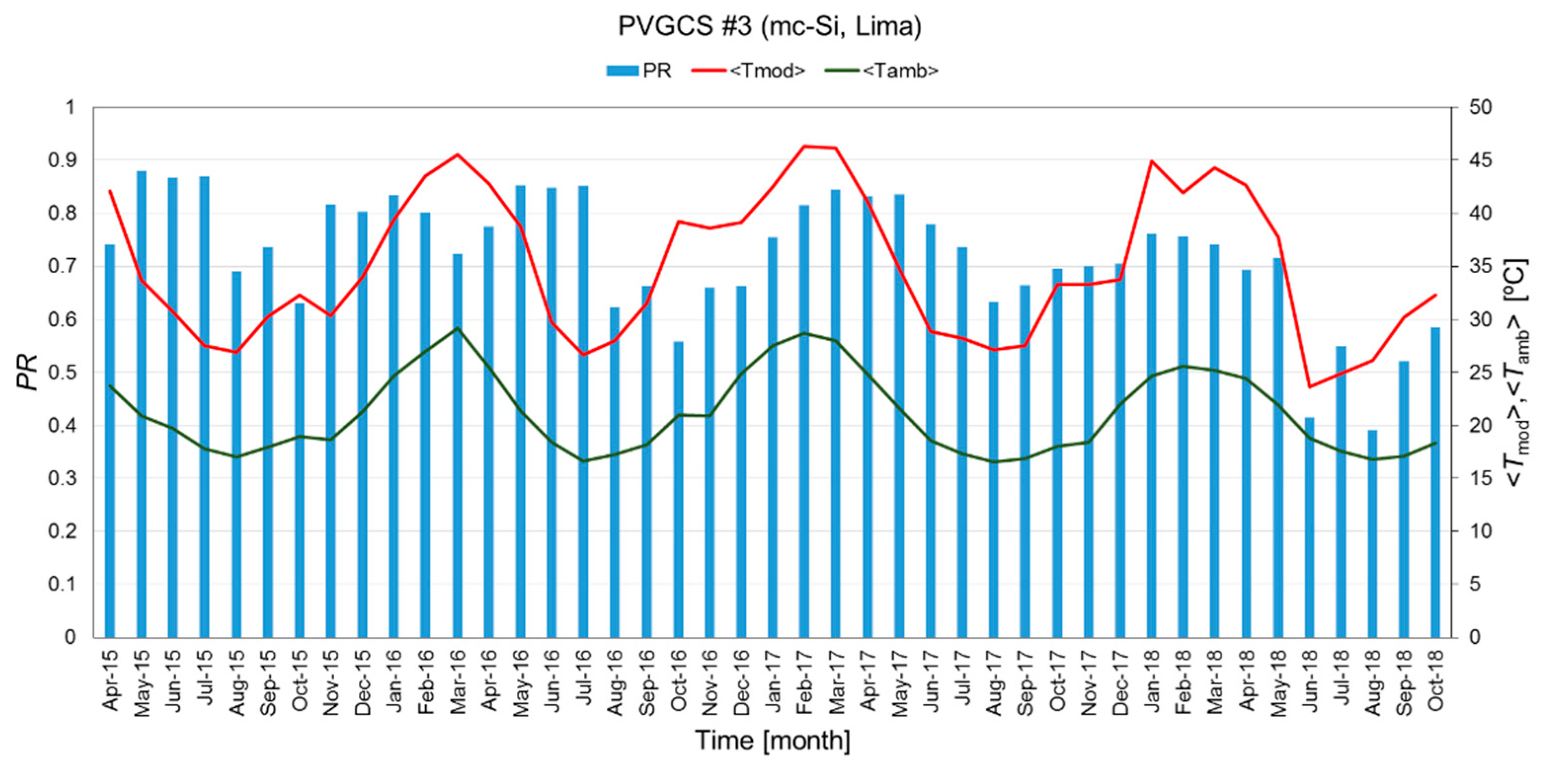
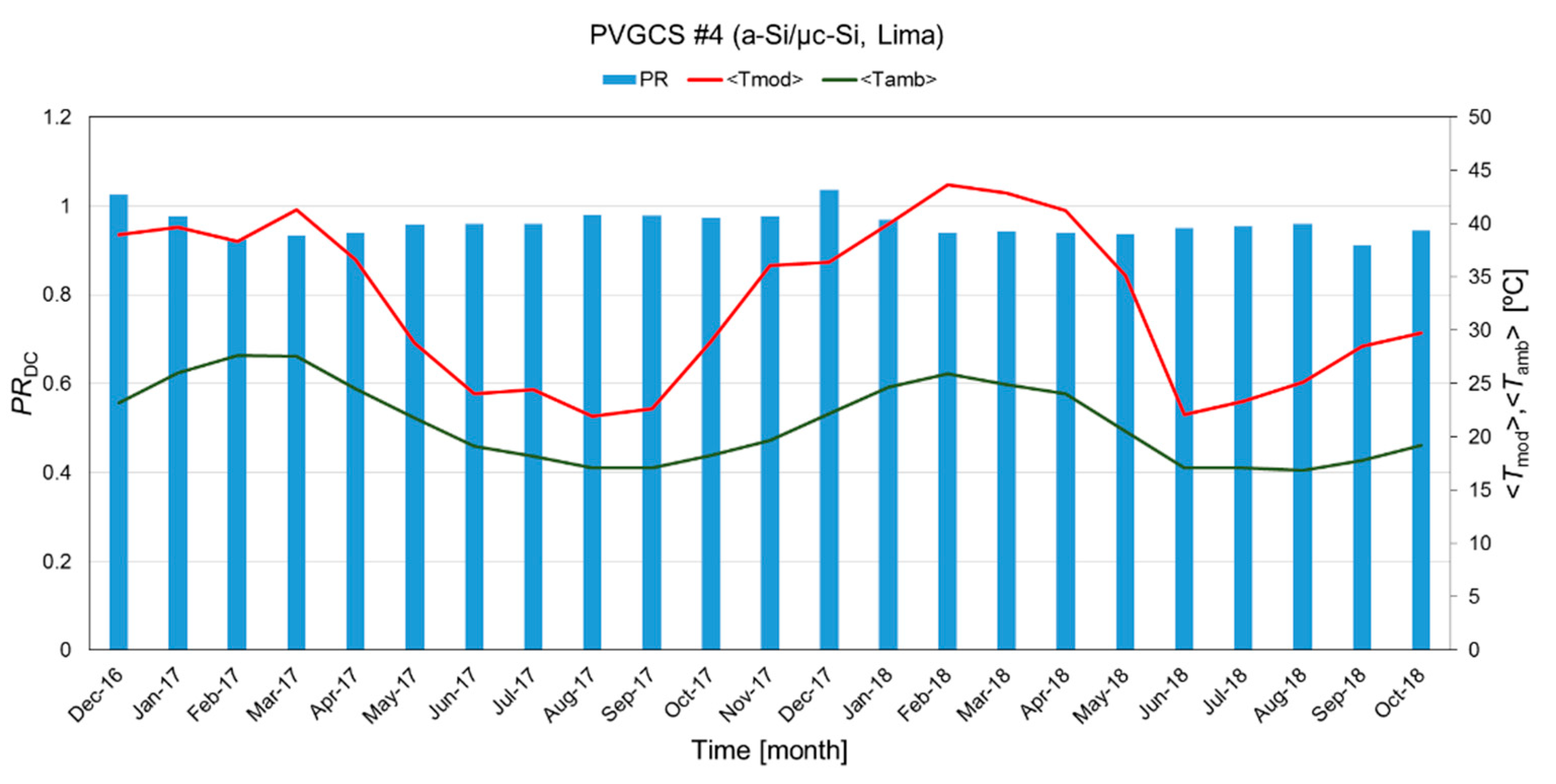
3.2. Monthly Performance Metrics

Figure 6, Figure 7 and Figure 8 show the values of PR for PVGCS #1–#3, while Figure 9 depicts the values of PRDC for PVGCS #4. All these values are plotted over the period under study of each system. In order to gain a better interpretation of the behavior of the four cases of study, ambient and module temperatures averaged on a monthly basis during daytime (<Tamb>, in °C and <Tmod>, in °C, respectively) are also shown in these Figures. The latter parameters are obviously correlated and help analyze the detrimental impact of the module temperature increase on PV performance.
Virtually no inverter shutdowns occurred in any system during the period under study. However, inverter clipping was very sporadically observed in Arequipa and Tacna in December-April and October-April, respectively. Inverter saturation was also identified in the a-Si/µc-Si PV system located in Lima during 2017—October and November—and April 2018. These losses are caused by the slight undersizing of the inverters relative to the PV field, as discussed in Section 2.1. Additionally, partial shadowing experienced by the PV field in Tacna during some autumn and winter months exerted a negative influence on its performance, as discussed below.
A fairly stable behavior of PVGCS #1 in terms of performance is noticeable in Figure 6. Although not monitored over the course of the experimental campaign, mild and steady wind flows play an important role in conjunction with not too extreme ambient temperatures in Arequipa to keep <Tmod> between 28–36 °C. The calculated values of PR show little fluctuation over the experimental campaign, since they lie between 0.80 and 0.91. As expected, higher/lower values of the latter parameter are related to lower/higher of values of <Tmod>.
The performance of PVGCS #2 shows a clearly noticeable seasonal trend. Thus, PR ranges from 0.70 to 0.88, as illustrated in Figure 7. Contrary to what might be expected, the latter parameter was lower in June and July than in other warmer months. Unfortunately, shortly after the PV system was installed in Tacna, a building was constructed in its vicinity. Partial shadowing losses were caused by this building in May-July, when the sun’s altitude was lower, as shown in Figure 10.
PVGCS #3 exhibits a remarkable seasonality, mainly caused by the influence of two factors described as follows. Higher module temperatures lower PR, thus decreasing it to 0.69 in April 2018. Conversely, PR lies within 0.87–0.88 in May–July 2016, when temperatures were colder. On the other hand, most in-plane irradiation was collected in Lima at low levels of in-plane irradiance (<200 W·m−2) in August-October, which is conducive to a remarkable decrease of PV efficiency. To achieve a better understanding of this phenomenon, a specific month of the latter interval was studied. Thus, the percent and accumulated percent of Hi in different ranges of Gi during August 2017 for PVGCS #3—whose PVRD was left unclean—and PVGCS #4—whose PVRD was cleaned on a weekly basis—are shown in Figure 11. Clearly, the distribution of Hi is remarkably enhanced at lower Gi classes, regardless of whether the in-plane irradiation comes from a weekly cleaned PVRD or a PVRD left unclean. As shown below, this leads to a poor performance of mc-Si PV modules, due to the losses this PV material exhibits at low irradiance levels. Specifically, for the month under scrutiny, as much as 65% of the in-plane irradiation was collected below 200 W·m−2, as measured with the weekly cleaned PVRD. This percentage rises up to over 70% when measured with the PVRD left unclean. By contrast, the portion of Hi collected below 200 W·m−2 shrinks to only some 10% in some warmer months, such as March 2016, as shown in Figure 11.
It is a well-known fact that the performance of a PV device decreases in a non-linear way at low light levels. It is worthy to mention a recently published study [41], in which the influence of the intensity of incident irradiance on the efficiency of various PV technologies was analyzed. In this publication, the normalized efficiency (ηeff) is defined as the ratio of the PV module efficiency—corrected at 25 °C and measured with a PVRD of the same technology as the PV module under test—to the PV module efficiency at STC. Thus, values of ηeff of 0.90 and 0.84 were found for a sc-Si module at 200 and 100 W·m−2, respectively. More specifically, Kenny et al. [42] gave 0.94 and 0.82 for ηeff at these two incident irradiance levels for a mc-Si PV module. It is clear that low irradiance losses exert a highly noticeable detrimental impact on the performance of mc-Si PV modules in Lima. However, the system must have experienced some other additional losses to justify the extraordinary low values of PR in June and August 2018, which lie in the vicinity of 0.4. Some further research is needed to look into this abnormally bad performance. Anyway, a clear steady decline in the PV system performance is noticeable in Figure 8, a fact that may suggest early degradation issues were underwent by mc-Si PV modules. Such a decline is to be quantified on an annual basis when values of PRannual over the years under scrutiny are shown hereafter in Section 3.3.
The performance of PVGCS #4 shows a scarcely seasonal profile, as illustrated in Figure 9. Indeed, values of PRDC lie between 0.94 and 1.03 over the period under study. As shown in Table 2, the lower maximum power temperature coefficient of a-Si/µc-Si PV modules makes them less vulnerable to the influence of the module temperature than those made of c-Si technologies. Moreover, the decrease of performance of this system due to low irradiance levels is far lower than that experienced by PVGCS #3, as PRDC stays above 0.94. Unfortunately, as far as we know, the behavior of a-Si/µc-Si PV modules under low levels of illumination has not been quantitatively addressed. However, Mavromatakis et al. [41] found values of ηeff of 0.98 and 0.94 for an amorphous silicon tandem PV module at 200 and 100 W·m−2. Such values might well be similar to those exhibited by a tandem a-Si/µc-Si PV module, thereby explaining the good performance of this technology at low irradiance levels.
Nevertheless, the overperformance of PVGCS #4 relative to PVGCS #3 should be taken with some caution. Even leaving aside the obvious lack of inverter losses influencing PRDC, spectral effects are likely to result in an overestimation of the latter parameter. No studies addressing the spectral distribution of irradiation in Lima were available at the time of this writing. However, seasonal variations of the solar spectrum are negligible in low latitude sites, such as Lima’s, given that the air mass at solar noon shows no substantial variations along the year [43,44,45]. Besides, predominant diffuse irradiance in Lima contributes to enhancing shorter wavelengths in spectral distributions. Consequently, blue-shifted spectra are hypothesized to prevail in Lima. If this were so, slight spectral gains could have been exhibited by a-Si/µc-Si PV modules [43], while slight spectral losses could have been undergone by the sc-Si irradiance sensor, thus leading to an overestimation of PRDC. Moreover, stabilization and long-term degradation issues of a-Si/µc-Si PV modules in coastal desert climates have not been thoroughly studied yet. By way of example, the stabilization period for this thin film material has been reported to last up to 14 months in Jaén (Spain) [46], a site with a continental-Mediterranean climate. It could have been the case that the PV modules of PVGCS #4 had not reached their steady state before the beginning of the period of study in December 2016. Consequently, further research on the above issues is needed to assess more accurately the performance of this PV technology in Lima.

3.3. Annual Yields and Annual Performance Ratio

Table 3 shows values of Yr,annual for the four systems investigated. Values of Yf,annual, in kWh·kW−1 for PVGCS #1–#3 as well as a single annual value of YA,annual for PVGCS #4 are also gathered in this Table. Consequently, values of annual performance ratio for each system—shown in Table 4—may be easily derived from the information contained in Table 3. It should be borne in mind that the period of analysis for PVGCS #1 extends from August 2015 to October 2018, while those of PVGCS #2 and #3 extend from May 2015–October 2018 and April 2015–October 2018, respectively. Likewise, PVGCS #4 was analyzed during the period of December 2016–October 2018 in this paper. However, the 12-month periods considered in both Tables start in August 2015 in order to evaluate the earlier parameters over the same time frames for all the PV systems studied in this paper.
Reporting annual values of Yr,annual may not be useful for PVGCS #1–#3, as such yields have been calculated by using effective irradiance, which might be largely decreased by the soiling level. Thus, given that neither the PV modules nor the PVRD are cleaned in these three systems, the scarcity of natural cleaning actors (rain) in desert climates—such as those of Arequipa, Tacna, and Lima—greatly raises the soiling impact on Gi records. Angular losses underwent by the PVRD are also enlarged by the deposition of soil and dust, as modeled by Martín and Ruiz [47,48]. However, it is worth noting that the PVRD of PVGCS #3 and PVGCS #4 were installed in the same site (Lima), some 1 km away from each other, and have the same tilt angle and orientation. As the PVRD of the latter system is cleaned weekly, an estimate of the annual losses experienced by the available effective irradiation for PVGCS #3 over the period of Aug 2017–Jul 2018 may be derived from the ratio of its annual reference yield to that calculated for PVGCS #4 for the same period (Table 3). Therefore, as much as 21% of potential PV generation is estimated to be lost due to leaving the PV field unclean, which is a far larger loss than those reported in more rainy and temperate climates [49].
Investigating the soiling impact is beyond the scope of this paper. Nevertheless, providing some results of previous contributions on the issue may help put in context the above estimate of the influence of soiling on the performance of PVGCS #3. Unfortunately, the literature on quantifying the potential PV generation losses in Latin American sites with arid climates is very rare and limited to Chile. Thus, Ferrada et al. [19] investigated values for the varying slope of daily time series of PR as a function of the soiling level for sc-Si and a-Si/µc-Si PV modules in a coastal desert climate site (Antofagasta, Chile), while Urrejola et al. [20] analyzed the impact of soiling on the degradation of sc-si, mc-Si, and a-Si/µc-Si PV modules in Santiago (Chile). However, neither contribution presents an estimate of annual losses caused by soiling. In this sense, some studies dealing on this topic in sites in the Persian Gulf region—some of which have desert coastal climates—are worthy of mentioning. Soiling PV losses up to 32% in eight months were reported in in Ryadh (Saudi Arabia) [50]. Some 70% of PV power was found to be lost in a year due to soiling issues in a site of the United Arab Emirates [51]. Another study carried out in Dahran (Saudia Rabia) found losses of 50% on a PV system during six months [52].
As discussed in Section 1, studies available in the literature on the performance of various photovoltaic technologies in different locations worldwide are informative, but often difficult to compare with each other and interpret properly. However, it is advisable to compare the results obtained in this paper with some of the studies reviewed in the earlier section that were conducted with identical or similar PV materials under reasonably similar climates and experimental protocols. In doing so, the analysis presented here is put in a broader perspective. In this sense, it is clear that the results of the operation of the sc-Si PV system of Arequipa slightly outperforms those reported for PVGCS in Soha (mc-Si, Oman) [15] and Kerman (mc-Si, Iran). The PV system located in Arequipa also outperforms the remaining three installations analyzed here and those studied in Mugla (sc-Si, Turkey) [16], Azda and Sawda (CIGS, Kuwait) [18], and Antofagasta (sc-Si, Chile) [19]. The values of Yf,annual achieved in Tacna stay not far below the average of the final yield of the three latter studies. However, the values of PRannual obtained in this site are only very slightly outperformed by those calculated here for Arequipa and by those reported for the PVGCS located in Soha and Kerman. Poor annual yields are achieved in both PVGCS installed in Lima, mainly due to its low irradiation resource when compared to Arequipa’s, Tacna’s, and those of the remaining sites described earlier. The values of PRannual for the mc-Si PV system in Lima during the period of August 2015–July 2016 (0.77) and August 2016–July 2017 (0.76) are similar to many of the cases reported in Section 1 although they remain below those achieved by the other two sc-Si PV systems evaluated here. Anyway, the noticeable drop in the performance experienced by this mc-Si system during August 2017–July 2018 (0.70) needs some further investigation. This remarkable decline of the values of PRannual may well suggest early degradation issues experienced by the PV field, as noted in the previous Section. Last, an astonishing value of 0.97 was reached by PRDC,annual in the thin film PV system. The presumably prevailing blue-rich solar spectrum of the low-latitude and overcast city of Lima may have led to small spectral gains experienced by a-Si/µc-Si PV modules. Such spectral gains, combined with small spectral losses underwent by the sc-Si PVRD, could have resulted in an overestimation of the PV array performance. In addition, the PV field may have not reached a steady state before the beginning of the analyzed period so that its actual power at STC could have been greater than the sum of the nameplate rating of its PV modules [46,53,54]. These two facts could partly explain this abnormally high value of PRDC,annual, but further research is also needed to investigate this issue.

4. Conclusions

Despite the growing contribution of PV to the electricity mix in Peru, no outdoor behavior data of this technology specific to this country are available in the literature. To overcome this lack of knowledge, a performance assessment of various PV module technologies (sc-Si, mc-Si, and a-Si/µc-Si), in three Peruvian sites with desert climates was carried out in this paper. A 3.3-kWp sc-Si PVGCS was installed in Arequipa and another identical system in Tacna. Both a 3-kWp mc-Si and a 3.5-kWp a-Si/µc-Si PVGCS were installed in Lima. The three c-Si PV systems were monitored during more than three years while the remaining thin film PV system was monitored for more than one and a half years. The sc-Si and mc-Si PV modules together with their sc-Si irradiance sensors were left unclean over the course of the experimental campaign whilst a PV subfield of the a-Si/µc-Si PVCS located in Lima was cleaned weekly in conjunction with its sc-Si irradiance sensor. Consequently, a proper estimation of soiling losses estimation was out of the scope of this paper as sc-Si irradiance sensors were kept in the same state of cleanliness as the PV modules under scrutiny.
Arequipa showed the highest effective solar resource and the most relatively stable monthly effective irradiation profile. This resulted in values of Yf,annual for the sc-Si PV system located in this site that lay between 1770 and 1992 kWh·kW−1. A more seasonal trend in the monthly reference and final yields was noticeable for the sc-Si PV system of Tacna, where Yf,annual ranged from 1537 to 1540 kWh·kW−1. The most variable and lowest effective irradiation profile occured in Lima. Obviously, this low solar resource of Lima resulted in values of Yf,annual that were between 736 and 833 kWh·kW−1 for the mc-Si PV system, while a value of 1338 kWh·kW−1 was found for YA,annual for the weekly cleaned a-Si/µc-Si PV system.
The analysis in terms of performance provides a more meaningful insight as no pyranometers were used, but sc-Si irradiance sensors, which were kept in the same state of cleanliness as the PV modules under scrutiny. Thus, smooth monthly fluctuations were experienced by PR for the PV system of Arequipa, thanks to the relatively smaller ambient temperature span combined with mild and steady wind flows. Indeed, PR varied between 0.80–0.91 and PRannual were in the vicinity of 0.84. Values of the latter parameter between 0.81 and 0.83 were obtained in Tacna for a twin sc-Si installation of the previous one. The detrimental influence of higher temperatures—relative to Arequipa—combined with partial shadowing, occurred during autumn and winter months in the PV system located in the latter site, leading to lower values of PR (0.70–0.88). It is worth noting that minor inverter clipping episodes occurred in both Arequipa and Tacna in December–April and October–April, respectively.
The most pronounced performance seasonality occurred in the mc-Si PV system studied in Lima. In addition to the drop caused in PR by higher temperatures, low irradiance losses exerted a highly noticeable negative impact on the outdoor behavior of mc-Si PV modules in August–October. PR peaked (0.88) in July 2016—a winter month—while this parameter lowered to 0.69 in a warm month, such as April 2018. Abnormally low values for this parameter—down to slightly below 0.4—were found in June and August 2018, which obviously need to be investigated further. As a result of the losses mentioned, this PV system performed worse than the previous two ones. Indeed, PRannual ranged from 0.70 to 0.77. A clear steady decline of the performance was noticeable in this mc-Si PV, which may suggest early PV module degradation issues. Future efforts will be aimed at periodically measuring I-V curves of these mc-Si PV modules and translating them to STC—using on-site procedures, such as that described by Nofuentes et al. [55]—to ascertain such degradation over time.
Regarding the a-Si/µc-Si PV subfield analyzed in Lima, PRDC showed the flattest profile as it was between 0.94 and 1.03 over the period under scrutiny. Such an excellent monthly behavior led to an outstanding annual performance, with a PRDC of 0.97. It is a well-known fact that this PV material is less influenced by temperature than c-Si. Moreover, a-Si/µc-Si appears to be far less influenced by low irradiance losses than mc-Si. Anyway, the accuracy of these good results should be taken cautiously as spectral effects experienced by both the sc-Si sensor and the PV subfield might have masked the calculations to some extent. Furthermore, stabilization periods, degradation rates, and metastabilities of thin film materials are issues that still remain elusive. Thus, the actual power of the PV subfield over the course of the experimental campaign might have been greater than that considered in the calculation of performance ratio, i.e., the sum of the nameplate rating of the a-Si/µc-Si PV modules.
Investigating the performance of some other PV materials in Peru is underway at present within the frame of the project, Evaluación energética y técnico-económica de la generación de energía eléctrica renovable con nuevas tecnologías fotovoltaicas en diferentes zonas climáticas del Perú (Energy and technical-economic assessment of the generation of renewable electric energy with new photovoltaic technologies in different climatic zones of Peru), funded by the Peruvian National Fund for Scientific and Technological Development & Technological Innovation in conjunction with the World Bank. Specifically, small PVGCS (<2 kW) using CIGS, heterojunction with intrinsic thin layer (HIT), and mono Passivated Emitter and Rear Cell (PERC) PV modules are to be installed during 2019 in various sites of Peru. Some promising and enlightening results are expected to be available after a three-year-long monitoring period. In this sense, foreseeing the PV performance of such technologies under the wide variety of climates existing in this Andean country may be adventurous, although some guesswork may be attempted. In this sense, no fairly good results are likely to be obtained using CIGS in Lima due to the presumably prevailing blue-rich spectra of this site—conducive to spectral losses in this PV material [56]—together with the low irradiance losses this technology exhibits [41]. By contrast, HIT modules are less vulnerable to the influence of temperature and low irradiance levels [41], which may result in a better performance of such PV technology in this site. HIT modules also seem to be well suited for desert climates with abundant solar resource [57]. Anyway, it is clear that some of the locations where these new PVGCS are to be installed combine high humidity levels with high temperatures, thus likely leading to an increase in the moisture ingress into modules, which in turn may result in a faster corrosion of solder bonds in mono PERC and HIT PV modules. Some corrosion phenomena might also take place in the transparent conductive oxide layer of CIGS PV modules.
To summarize, according to the results obtained, sc-Si and presumably mc-Si PV modules are suitable to be used in desert climates, such as that of Arequipa, where environmental parameters keep monthly average module temperatures relatively low. Due to their fairly good performance, sc-Si and presumably mc-Si PV modules are also recommended for Tacna, a site with a desert climate with coastal influence. However, the detrimental impact of high temperature and low irradiance losses on the performance of mc-Si and, presumably, sc-Si PV modules discourages their use in Lima. Indeed, this is a site with a peculiar highly humid coastal desert climate, in which its low irradiation resource is collected at low irradiance levels during some winter months. Instead, a-Si/µc-Si PV technology makes the most of the comparatively scarce solar resource of Lima, as the efficiency of this thin film material is less influenced by both temperature and low light levels. Anyway, long-term performance of sc-Si, mc-Si, and thin-film PV technologies in Lima requires further research.

Author Contributions

I.R.-F. and G.N. wrote the manuscript. I.R.-F. filtered and processed the data. E.M.-C. and J.d.l.C. designed the PV installations and the monitoring systems. R.E.-P. performed operation and maintenance tasks of the PV installations. G.N. carried out the scientific supervision of the manuscript. J.d.l.C. was the principal researcher of the project that originated the results shown. All authors were involved in the analysis of data and the final preparation of the manuscript.

Funding

This research was funded by the Agencia Andaluza de Cooperación Internacional para el Desarrollo of the Junta de Andalucía (Andalusian Autonomous Government), within the frame of the project Emergiendo con el Sol. Apoyo institucional al Centro de Energías Renovables de la Universidad Nacional de Ingeniería de Lima (Perú) en el campo de la generación de energía eléctrica empleando tecnología fotovoltaica under expedient code 2012DEC026.

Acknowledgments

The authors are especially grateful to the researchers of the IDEA research group, the National University of San Agustín in Arequipa, the National University of Jorge Basadre Grohmann in Tacna and the National University of Engineering in Lima.

Conflicts of Interest

The authors declare no conflict of interest.

Abbreviations

Terminology
ACAlternating current
AfTropical rainforest climate
AmTropical monsoon climate
a-SiAmorphous silicon
a-Si/µc-SiAmorphous silicon/microcrystalline silicon heterojunction
AwTropical savanna climate
BshHot semi-arid climate
BskCold semi-arid climate
BwhHot desert climate
BwKCold desert climate
CfbOceanic climate
CIGSCopper indium gallium selenide
c-SiCrystalline silicon
CWbSubtropical highland climate
DCDirect current
GDPGross Domestic Product
HITHeterojunction with intrinsic thin layer
IECInternational Electrotechnical Commission
mc-SiPolycrystalline silicon
OsinergminPeruvian Supervisory Agency of Investment on Energy and Mining
PERCPassivated Emitter and Rear Cell
PVPhotovoltaic(s)
PVGCSPhotovoltaic grid-connected system
PVRDPhotovoltaic reference device
RTDResistive thermal detectors
sc-SiMonocrystalline silicon
STCStandard Test Conditions
Symbols
AaTotal module area (m2)
EAMonthly DC energy (Wh)
EoutMonthly PV module AC output (Wh)
GiMonthly in-plane irradiance (W·m−2)
Gi,kk-th recorded value of the in-plane irradiance (W·m−2)
G*Reference in-plane irradiance (1000 W·m−2)
HiMonthly in-plane irradiation (Wh·m−2)
mNumber of instances recorded during a month
PA (Gi, 25 °C)Power output of the PV field corrected at 25 °C (W)
PA,kk-th recorded value of the input DC power (W)
PoutOutput AC power (W)
Pout,kk-th recorded value of the output AC power (W)
P0PV module rating (W)
PRMonthly performance ratio
PRannualAnnual performance ratio
PRDCMonthly DC performance ratio
PRDC,annualAnnual DC performance ratio
TambAmbient temperature (°C)
TmodModule temperature (°C)
YAMonthly PV array energy yield (Wh·W−1)
YA,annualAnnual PV array energy yield (Wh·W−1)
YfMonthly final PV system yield (Wh·W−1)
Yf,annualAnnual final PV system yield (Wh·W−1)
YrMonthly reference yield (Wh·W−1)
Yr,annualAnnual reference yield (Wh·W−1)
ηeffNormalized efficiency
τkDuration of the k-th recording interval (h)

References

  1. Fraunhofer ISE. Available online: https://www.ise.fraunhofer.de/content/dam/ise/de/documents/publications/studies/Photovoltaics-Report.pdf (accessed on 7 December 2018).
  2. Photon International. Markets worldwide. The Solar Power Magazine, September 2018; no. 9. 8. [Google Scholar]
  3. Erge, T.; Hoffmann, V.U.; Kiefer, K. The German experience with grid-connected PV-systems. Solar Energy 2001, 70, 479–487. [Google Scholar] [CrossRef]
  4. Pietruszko, S.M.; Gradzki, M. Performance of a grid connected small PV system in Poland. Appl. Energy 2003, 74, 177–184. [Google Scholar] [CrossRef]
  5. Hontoria, L.; Aguilera, J.; Almonacid, F.; Nofuentes, G.; Zufiria, P. Artificial Intelligence in Energy and Renewable Energy Systems; Kalogirou, S., Ed.; Nova Publishers Inc.: Chichester, UK, 2006; pp. 163–200. [Google Scholar]
  6. Muñoz, F.J.; Almonacid, G.; Nofuentes, G.; Almonacid, F. A new method based on charge parameters to analyse the performance of stand-alone photovoltaic systems. Sol. Energy Mater. Sol. Cells 2006, 90, 1750–1763. [Google Scholar] [CrossRef]
  7. Bakos, G.C. Distributed power generation: A case study of small scale PV power plant in Greece. Appl. Energy 2009, 86, 1757–1766. [Google Scholar] [CrossRef]
  8. Zou, X.; Li, B.; Zhai, Y.; Liu, H. Performance monitoring and test system for grid-connected photovoltaic systems. In Proceedings of the 2012 Asia-Pacific Power and Energy Engineering Conference, Shanghai, China, 27–29 March 2012. [Google Scholar]
  9. Congedo, P.M.; Malvoni, M.; Mele, M.; De Giorgi, M.G. Performance measurements of monocrystalline silicon PV modules in South-eastern Italy. Energy Convers. Manag. 2013, 68, 1–10. [Google Scholar] [CrossRef]
  10. Micheli, D.; Alessandrini, S.; Radu, R.; Casula, I. Analysis of the outdoor performance and efficiency of two grid connected photovoltaic systems in northern Italy. Energy Convers. Manag. 2014, 80, 436–445. [Google Scholar] [CrossRef]
  11. Adaramola, M.S.; Vågnes, E.E.T. Preliminary assessment of a small-scale rooftop PV-grid tied in Norwegian climatic conditions. Energy Convers. Manag. 2015, 90, 458–465. [Google Scholar] [CrossRef]
  12. Milosavljević, D.D.; Pavlović, T.M.; Piršl, D.S. Performance analysis of A gridconnected solar PV plant in Niš, republic of Serbia. Renew. Sustain. Energy Rev. 2015, 44, 423–435. [Google Scholar] [CrossRef]
  13. Phinikarides, A.; Makrides, G.; Zinsser, B.; Schubert, M.; Georghiou, G.E. Analysis of photovoltaic system performance time series: Seasonality and performance loss. Renew. Energy 2015, 77, 51–63. [Google Scholar] [CrossRef]
  14. De Prada-Gil, M.; Domínguez-García, J.L.; Trilla, L.; Gomis-Bellmunt, O. Technical and economic comparison of various electrical collection grid configurations for large photovoltaic power plants. IET Renew. Power Gener. 2017, 11, 226–236. [Google Scholar] [CrossRef]
  15. Kazem, H.A.; Khatib, T.; Sopian, K.; Elmenreich, W. Performance and feasibility assessment of a 1.4 kW roof top grid-connected photovoltaic power system under desertic weather conditions. Energy Build. 2014, 82, 123–129. [Google Scholar] [CrossRef]
  16. Eke, R.; Demircan, H. Performance analysis of a multi crystalline Si photovoltaic module under Mugla climatic conditions in Turkey. Energy Convers. Manag. 2013, 65, 580–586. [Google Scholar] [CrossRef]
  17. Edalati, S.; Ameri, M.; Iranmanesh, M. Comparative performance investigation of mono- and poly-crystalline silicon photovoltaic modules for use in grid-connected photovoltaic systems in dry climates. Appl. Energy 2015, 160, 255–265. [Google Scholar] [CrossRef]
  18. Al-Otaibi, A.; Al-Qattan, A.; Fairouz, F.; Al-Mulla, A. Performance evaluation of photovoltaic systems on Kuwaiti schools’ rooftop. Energy Convers. Manag. 2015, 95, 110–119. [Google Scholar] [CrossRef]
  19. Ferrada, P.; Araya, F.; Marzo, A.; Fuentealba, E. Performance analysis of photovoltaic systems of two different technologies in a coastal desert climate zone of Chile. Solar Energy 2015, 114, 356–363. [Google Scholar] [CrossRef]
  20. Urrejola, E.; Antonanzas, J.; Ayala, P.; Salgado, M.; Ramírez-Sagner, G.; Cortés, C.; Pino, A.; Escobar, R. Effect of soiling and sunlight exposure on the performance ratio of photovoltaic technologies in Santiago, Chile. Energy Convers. Manag. 2016, 114, 338–347. [Google Scholar] [CrossRef]
  21. Kottek, M.; Grieser, J.; Beck, C.; Rudolf, B.; Rubel, F. World map of the Köppen–Geiger climate classification updated. Meteorol. Z. 2006, 15, 259–263. [Google Scholar] [CrossRef]
  22. The World Bank. Available online: http://www.worldbank.org/en/country/peru/overview (accessed on 4 December 2018).
  23. International Energy Agent. Available online: https://www.iea.org/statistics (accessed on 11 December 2018).
  24. Zambrano-Monserrate, M.A.; Silva-Zambrano, C.A.; Davalos-Penafiel, J.L.; Zambrano-Monserrate, A.; Ruano, M.A. Testing environmental Kuznets curve hypothesis in Peru: The role of renewable electricity, petroleum and dry natural gas. Renew. Sustain. Energy Rev. 2018, 82, 4170–4178. [Google Scholar] [CrossRef]
  25. Photon International. Markets worldwide. The Solar Power Magazine, May 2018; no. 5. 22. [Google Scholar]
  26. Osinergmin. Available online: https://www.osinergmin.gob.pe/ (accessed on 5 December 2018). (In Spanish).
  27. SolarPack. Available online: https://www.solarpack.es/pais/peru/ (accessed on 5 December 2018). (In Spanish).
  28. Martinez-Plaza, D.; Abdallah, A.; Figgis, B.W.; Mirza, T. Performance improvement techniques for photovoltaic systems in Qatar: Results of first year of outdoor exposure. Energy Procedia 2015, 77, 386–396. [Google Scholar] [CrossRef]
  29. European Commission. Available online: http://re.jrc.ec.europa.eu/pvg_tools/en/tools.html (accessed on 10 November 2018).
  30. PVSYST. Available online: http://www.pvsyst.com/en/ (accessed on 20 September 2018).
  31. Nasa Prediction of Wordlwide Energy Resources. Available online: https://eosweb.larc.nasa.gov/sse/ (accessed on 10 November 2018).
  32. Nofuentes, G.; Almonacid, G. Design tools for the electrical configuration of architecturally-integrated PV in buildings. Prog. Photovolt. Res. Appl. 1999, 7, 475–488. [Google Scholar] [CrossRef]
  33. Muñoz, J.V.; Nofuentes, G.; Aguilera, J.; Fuentes, M.; Vidal, P.G. Procedure to carry out quality checks in photovoltaic grid-connected systems: Six cases of study. Appl. Energy 2011, 88, 2863–2870. [Google Scholar] [CrossRef]
  34. IEC 61724-1:2017. Photovoltaic System Performance Monitoring—Guidelines for Measurement, Data Exchange and Analysis; IEC Standard; IEC: Geneva, Switzerland, 2017. [Google Scholar]
  35. Dunn, L.; Gostein, M.; Emery, K. Comparison of pyranometers vs. PV reference cells for evaluation of PV array performance. In Proceedings of the 38th IEEE Photovoltaic Specialists Conference, Austin, TX, USA, 3–8 June 2012. [Google Scholar]
  36. Osterwald, C.R.; Emery, K.A.; Muller, M. Photovoltaic module calibration value versus optical air mass: The air mass function. Prog. Photovolt. Res. Appl. 2012, 22, 560–573. [Google Scholar] [CrossRef]
  37. Caballero, J.A.; Fernández, E.F.; Theristis, M.; Almonacid, F.; Nofuentes, G. Spectral Corrections Based on Air Mass, Aerosol Optical Depth, and Precipitable Water for PV Performance Modeling. IEEE J. Photovolt. 2018, 8, 552–558. [Google Scholar] [CrossRef]
  38. Ye, J.Y.; Reindl, T.; Aberle, A.G.; Walsh, T.M. Performance degradation of various PV module technologies in tropical Sigapore. IEEE J. Photovolt. 2014, 4, 1288–1294. [Google Scholar] [CrossRef]
  39. Ozden, T.; Akinoglu, B.G.; Turan, R. Long term outdoor performances of three different on-grid PV arrays in central Anatolia—An extended analysis. Renew. Energy 2017, 101, 182–195. [Google Scholar] [CrossRef]
  40. De Parra, I.; Muñoz, M.; Lorenzo, E.; García, M.; Marcos, J.; Martínez-moreno, F. PV performance modelling: A review in the light of quality assurance for large PV plants. Renew. Sustain. Energy Rev. 2017, 78, 780–797. [Google Scholar] [CrossRef]
  41. Mavromatakis, F.; Vignola, F.; Marion, B. Low irradiance losses of photovoltaic modules. Solar Energy 2017, 157, 496–506. [Google Scholar] [CrossRef]
  42. Kenny, R.P.; Vigano, D.; Salis, E.; Bardizza, G.; Norton, M.; Müllejans, H.; Zaaiman, W. Power rating of photovoltaic modules including validation of procedures to implement IEC61853-1 on solar simulators and under natural sunlight. Prog. Photovolt. Res. Appl. 2013, 21, 1384–1399. [Google Scholar] [CrossRef]
  43. Ye, J.Y.; Reindl, T.; Aberle, A.G.; Walsh, T.M. Effect of solar spectrum on the performance of various thin-film PV module technologies in tropical Singapore. IEEE J. Photovolt. 2014, 4, 1268–1274. [Google Scholar] [CrossRef]
  44. Amillo, A.M.G.; Huld, T.; Vourlioti, P.; Müller, R.; Norton, M. Application of Satellite-Based Spectrally-Resolved Solar Radiation Data to PV Performance Studies. Energies 2015, 8, 3455–3488. [Google Scholar] [CrossRef]
  45. Nofuentes, G.; de la Casa, J.; Solís-Alemán, E.M.; Fernández, E.F. Spectral impact on PV performance in mid-latitude sunny inland sites: Experimental vs. modelled results. Energy 2017, 141, 1857–1868. [Google Scholar] [CrossRef]
  46. Kichou, S.; Abaslioglu, E.; Silvestre, S.; Nofuentes, G.; Torres-Ramírez, M.; Chouder, A. Study of degradation and evaluation of model parameters of micromorph silicon photovoltaic modules under outdoor long term exposure in Jaén, Spain. Energy Convers. Manag. 2016, 120, 109–119. [Google Scholar] [CrossRef]
  47. Martin, N.; Ruiz, J. Calculation of the PV modules angular losses under field conditions by means of an analytical model. Sol. Energy Mater. Sol. Cells 2001, 70, 25–38. [Google Scholar] [CrossRef]
  48. Martin, N.; Ruiz, J. Corrigendum to calculation of the PV modules angular losses under field conditions by means of an analytical model. Sol. Energy Mater. Sol. Cells 2013, 110, 154. [Google Scholar] [CrossRef]
  49. Costa, S.C.S.; Diniz, A.S.A.C.; Kazmerski, L.L. Solar energy dust and soiling R&D progress: Literature review update for 2016. Renew. Sustain. Energy Rev. 2018, 82, 2504–2536. [Google Scholar]
  50. Salim, A.; Huraib, F.; Eugenio, N. PV power-study of system options and optimization. In Proceedings of the 8th European PV Solar Energy Conference, Florence, Italy, 9–13 May 1988. [Google Scholar]
  51. Al-Sabounchi, A.; Yalyali, S.; Al-Thani, H. Design and performance evaluation of a photovoltaic grid-connected system in hot weather conditions. Renew. Energy 2013, 53, 71–78. [Google Scholar] [CrossRef]
  52. Adinoyi, M.; Said, S. Effect of dust accumulation on the power outputs of solar photovoltaic modules. Renew. Energy 2013, 60, 633–636. [Google Scholar] [CrossRef]
  53. Jordan, D.C.; Kurtz, S.R.; Vansant, K.; Newmiller, J. Compendium of photovoltaic degradation rates. Prog. Photovolt. Res. Appl. 2016, 24, 978–989. [Google Scholar] [CrossRef]
  54. Schweiger, M.; Bonilla, J.; Herrmann, W.; Gerber, A. Performance stability of photovoltaic modules in different climates. Prog. Photovolt. Res. Appl. 2017, 25, 968–981. [Google Scholar] [CrossRef]
  55. Nofuentes, G.; Aguilera, J.; Santiago, R.L.; de la Casa, J.; Hontoria, L. A reference-module-based procedure for outdoor estimation of crystalline silicon PV module peak power. Prog. Photovolt. Res. Appl. 2006, 14, 77–87. [Google Scholar] [CrossRef]
  56. Nofuentes, G.; de la Casa, J.; Torres-Ramírez, M.; Alonso-Abella, M. Solar spectral and module temperature influence on the outdoor performance of thin film PV modules deployed on a sunny inland site. Int. J. Photoenergy 2013, 2013, 620127. [Google Scholar] [CrossRef]
  57. Abdallah, A.; Martinez, D.; Figgis, B.; El Daif, O. Performance of Silicon Heterojunction Photovoltaic modules in Qatar climatic conditions. Renew. Energy 2016, 97, 860–865. [Google Scholar] [CrossRef]
Figure 1. Photographs of the PV systems under investigation. (Top left) PVGCS #1 in Arequipa (sc-Si, installation on flat roof); (top right) PVGCS #2 in Tacna (sc-Si, building integrated installation); (bottom left) PVGCS #2 in Lima (mc-Si, on-ground installation); (bottom right) PVGCS #4 in Lima (a-Si/µc-Si, on-ground installation).
Energies 12 00186 g001
Figure 2. Values of Yr and Yf for PVGCS #1 over the period under scrutiny. Both the PV field and PVRD were left unclean.
Energies 12 00186 g002
Figure 3. Values of Yr and Yf for PVGCS #2 over the period under scrutiny. Both the PV field and PVRD were left unclean.
Energies 12 00186 g003
Figure 4. Values of Yr and Yf for PVGCS #3 over the period under scrutiny. Both the PV field and PVRD were left unclean.
Energies 12 00186 g004
Figure 5. Values of Yr and YA for PVGCS #4 over the period under scrutiny. Both the PV subfield and PVRD were cleaned on a weekly basis.
Energies 12 00186 g005
Figure 6. Values of PR, <Tamb>, and <Tmod> for PVGCS #1 over the period under scrutiny. N.B. only values of temperature recorded during daytime are considered in the calculations.
Energies 12 00186 g006
Figure 7. Values of PR, <Tamb>, and <Tmod> for PVGCS #2 over the period under scrutiny. N.B. only values of temperature recorded during daytime are considered in the calculations.
Energies 12 00186 g007
Figure 8. Values of PR, <Tamb>, and <Tmod> for PVGCS #3 over the period under scrutiny. N.B. only values of temperature recorded during daytime are considered in the calculations.
Energies 12 00186 g008
Figure 9. Values of PRDC, <Tamb>, and <Tmod> for PVGCS #4 over the period under scrutiny. N.B. only values of temperature recorded during daytime are considered in the calculations.
Energies 12 00186 g009
Figure 10. Values of the power output of the PV field of PVGCS #2 corrected at 25 °C (PA[Gi, 25 °C], in W) vs. in-plane irradiance over a full day (06/28/2016). The sublinear behavior clearly distinguished between 300 and 800 W·m−2 is caused by a shade cast over the PV field. The shading impact of a surrounding element on the PV output is also noticeable below 200 W·m−2.
Energies 12 00186 g010
Figure 11. Percent and accumulated percent of Hi (Hi,cumul, in %) in different ranges of Gi during March 2016 for PVGCS #3 (top left), March 2016 for PVGCS#4 (top right), August 2017 for PVGCS #3 (bottom left), and August 2017 for PVGCS #4 (bottom right).
Energies 12 00186 g011
Table 1. Annual average values of some relevant meteorological parameters recorded in Arequipa, Lima, and Tacna.
Meteorological parameterArequipaTacnaLima
Horizontal irradiation (kWh·m−2) [29]238022801740
Ambient temperature (°C) [30]12.916.718.5
Minimum ambient temperature (°C) [31]8.113.418.8
Maximum ambient temperature (°C) [31]3231.518.9
Table 2. Values of the main electrical characteristics of the PV fields of the systems under investigation according to the manufacturer’s data sheets.
Electrical parameterPVGCS #1 and #2 (Arequipa and Tacna, sc-Si)PVGCS #3
(Lima, mc-Si)
PVGCS #4 1
(Lima, a-Si/µc-Si)
Maximum power at STC (W)330030102304
Short-circuit current at STC (A)8.986.9
Open-circuit voltage at STC (V)460511538
Module maximum power Temperature coefficient (°C−1)−0.0045−0.0045−0.0024
1 Only the PV subfield comprising two strings of a-Si/µc-Si PV modules connected in parallel to one of the inverter inputs is considered in this analysis.
Table 3. Values of annual yields (kWh·kW−1) for the four systems under study.
PeriodPVGCS #1 (Arequipa, sc-Si)
Yf,annual/Yr,annual
PVGCS #2
(Tacna, sc-Si)
Yf,annual/Yr,annual
PVGCS #3
(Lima, mc-Si)
Yf,annual/Yr,annual
PVGCS #4
(Lima, a-Si/µc-Si)
YA,annual/Yr,annual 1
Aug 2015–Jul 20161992/23431505/1792833/1082-
Aug 2016–Jul 20171770/21071537/1852778/1023-
Aug 2017–Jul 20181860/22141540/1855736/10901338/1380
1 Annual values of Yf for PVGCS #4 were not computed, as only one PV subfield connected to one of the inverter inputs is considered in the analysis.
Table 4. Values of PR,annual for PVGCS #1–#3 and PRDC,annual for PVGCS #4.
PeriodPVGCS #1
(Arequipa, sc-Si)
PVGCS #2
(Tacna, sc-Si)
PVGCS #3
(Lima, mc-Si)
PVGCS #4
(Lima, a-Si/µc-Si)
Aug 2015–Jul 20160.850.830.77-
Aug 2016–Jul 20170.840.820.76-
Aug 2017-Jul 20180.840.810.700.97

