On Modelling Wind-Farm Wake Turbulence Autospectra and Coherence from a Database

Abstract

This study addresses the feasibility of modeling wind-farm wake-turbulence autospectra and coherences from a database: flow velocity points from experimental and computational fluid dynamics (CFD) investigations. Specifically, it first applies an earlier-exercised framework to construct the autospectral models from a database and then it adopts a recently proposed framework to construct the coherence models from a database. While this proposed framework has not been tested against a database, the methodology has been completely formulated with a theoretical basis. These models of autospectrum and coherence are interpretive, and in closed form. Both frameworks basically involve the perturbation series expansion of the autospectra and coherences. The framework for modeling autospectra is tested against a demanding database of wake turbulence inside a wind farm over a complex terrain from a full-scale test. The suitability of these autospectral models for simulation through white-noise driven filters is also demonstrated. Finally, coherence models are generated for assumed values of the perturbation series constants, and these coherence models are used to demonstrate how the coherence models of homogeneous isotropic turbulence deviate from the coherence models of non-homogeneous non-isotropic turbulence such as wind-farm wake turbulence. This feasibility of extracting both the one-point statistics of autospectral models and the two-point statistics of coherence models from a database represents a research avenue that is new and promising in the treatment of wind-farm wake turbulence. This paper also demonstrates the feasibility of fruitfully exploiting the wake treatment methods developed in other fields.

1. Introduction

During the past thirty years, wake turbulence and its effects on wind turbines and wind farms have been extensively investigated, primarily analytically and to some extent experimentally. The extensive literature up to 2010 has been well covered in the widely used text of Manwell et al. [1]. As for the extensive analytical investigations since, suffice it to mention, as representative samples, Keck et al. [2] for wake-turbulence modeling from the low-fidelity CFD treatment of the Navier-Stokes (NS) equations, and Carrion et al. [3] for wake-turbulence modeling from the high-fidelity treatment of NS equations. The work of Carrion et al. [3] for example, includes a concise account of the state of the art of modeling wind-farm wake turbulence.

An overview of these investigations [1,2,3] is included here; although extremely brief, this should help appreciate how the present work serves as a desirable adjunct of experimental and high-fidelity CFD based investigations, and why it represents a new and promising avenue of wake-turbulence modeling. Wake-turbulence modeling falls into three categories:

• Semi-empirical models: These models are based on conservation of momentum and such simplified assumptions; and they typically contain an empirical constant. For example, the widely used model due to Katic et al. [1] belongs to this category; therein, the empirical constant is referred as wake decay constant. A recent work of Ge M. et al. [4] merits mention: it gives a thorough account of the key features of this class of models and their continual evolution as well as their utility base in the treatment of wind energy applications such as design of wind-farm layout.
• Low-fidelity CFD solutions: Several numerical schemes have been continually proposed (e.g., dynamic wake meandering model [2]); these are based on a wide range of physics-based approximations to NS equations. As more and more experimental databases become available, they are being continually updated and they merit further validation.
• High-fidelity CFD solutions: Despite the severe CPU-hour constraint, these high-fidelity approaches are indispensable in generating a database that serves as a reference point and in supplementing databases from experiments.

While major strides have been made in generating databases and in providing a much-improved understanding of wake turbulence, the current capability for modeling the one-point statistics of autospectrum, much more so, for modeling the two-point statistics of coherence, merits significant improvement. In fact, empirical exponential coherence functions are still being used [1]. Accordingly, the present study explores the feasibility of extracting the one-point statistics of autospectrum and the two-point statistics of coherence from a database.

The autospectral model extraction from a database of the present study is based on the framework due to Schau, Gaonkar and Polsky [5]. This framework guarantees that the extracted model and the autospectral data points have the same mean square value (a measure of turbulence energy), time scale and the Kolmogorov −5/3 spectral decay. For completeness, an earlier study by Gaonkar [6] should be mentioned as well; therein, the autospectral model extraction from a database is based on the framework of reference [7], in which the −5/3 spectral law is bypassed. Now it is expedient to address the development of a framework for extracting the two-point statistics models from a database. This can be approached either through cross-spectrum, which is a complex quantity involving the magnitude and phase or through coherence, which, as a spectral correlation coefficient, is a real quantity. The first approach generally leads to modeling the magnitude and not the phase, as was the case in Ref. [7]. The second approach through coherence is relatively more convenient and provides a means of capturing the two-point statistics from a database completely. The recent study due to Krishnan and Gaonkar [8] follows this second approach; although not tested against a database, the framework is formulated with a mathematical basis and the present study adopts this framework [8].

By design, these autospectral and coherence models are in closed form and they have a simple analytical structure to facilitate interrogation and interpretation of voluminous data points on autospectra and coherences. And they lend themselves well to routine use as a predictive tool. Compared to a description through such voluminous, numerically generated, autospectral and coherence data points, they describe wake turbulence analytically with better transparency and bring better understanding. Thus, these interpretive models broaden the scope and utility base of the database that invariably involves enormous resources. While the extracted models are database-specific (thus they are not predictive by themselves), the framework can be applied to any database and the model extraction is a routine exercise.

In the treatment of coherence for homogeneous isotropic turbulence for which the frozen turbulence hypothesis is applicable (HIT), the present study is motivated by and built on the earlier studies of Burton et al. [9], Houbolt and Sen [10], Frost et al. [11] and Irwin [12]. This treatment of coherence for HIT is found to show differences among these studies [9,10,11,12], and the present study, after an in-depth examination, follows Frost et al. [10] for cross-spectra and Irwin [12] for coherences. Given this background, the present study seems to provide a unified account of coherence for HIT in the treatment of wake turbulence.

To sum up: These interpretive models complement the experimental and CFD-based investigations as surrogate analytical models for both the one-point statistics of autospectrum and the two-point statistics of coherence. Moreover, this paper also demonstrates the feasibility of fruitfully exploiting the methodologies from other fields to the treatment of wind-turbine wake turbulence. And these methodologies offer promise towards providing a foothold on a formidably complex flow field inside a windfarm for engineering analysis.

Basic of Modeling

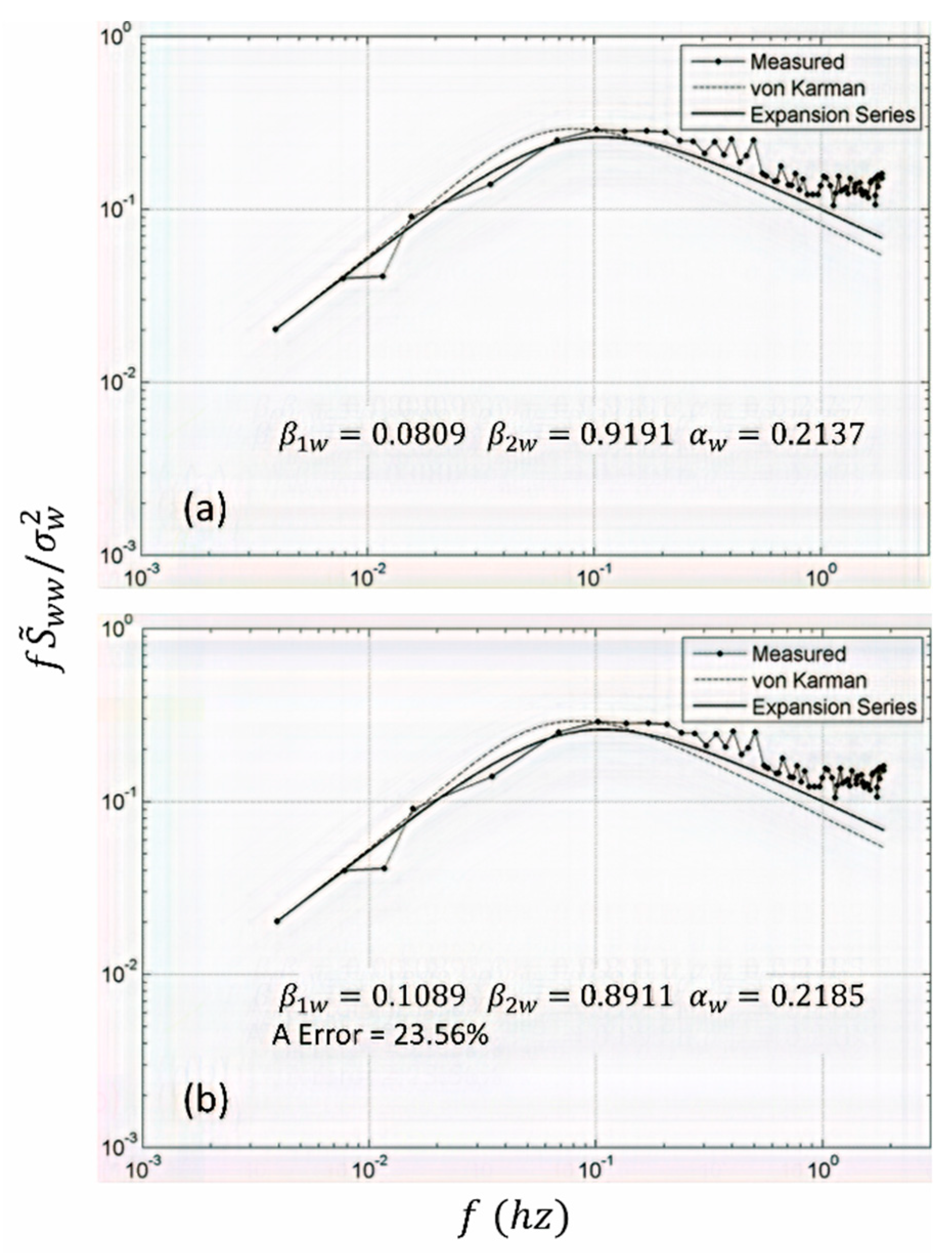
A comparison of the measured autospectra of ambient atmospheric boundary layer turbulence (ABL) and wake turbulence shows that the ABL autospectrum has gone through changes in energy distribution with respect to frequency. Figure 1 [13] should help bring a better understanding of this comparison; specifically, it shows measured dimensionless longitudinal autospectrum $f{\check{S}}_{uu}$/${\sigma }_u^2$ versus dimensionless frequency $fz$/$U$, where $z$ is the mast height and $U$ is the mean wind speed. These autospectra were experimentally generated at the same location in a wind farm over a complex terrain. Figure 1a refers to ABL with a turbulence intensity of 0.103, when the turbines were under stand-still conditions. Furthermore, Figure 1b refers to wake turbulence with a turbulence intensity of 0.204, when the turbines were fully operational. This change in the shape of the wake turbulence autospectrum cannot be realized through a linear superposition of a series of independently occurring changes at different frequencies on the ABL autospectrum. Thus, the autospectral morphing must be due to a nonlinear transformation of ABL. Stated otherwise, wind-farm wake turbulence could be idealized as nonlinearly transformed ABL and in turn, an earlier-developed mathematical framework for autospectral modeling of airwake-downwash turbulence could be adapted to modeling wind-farm wake turbulence as well [5,14]. (Airwake-downwash turbulence refers to the coupled flow-field of ship’s airwake shed from the superstructure and the helicopter downwash. Therein [5,14], the mathematical framework “posits” that airwake-downwash turbulence is nonlinearly transformed ABL. Regarding the coherence, the framework of Ref. 8 is adopted with the same justification that is used for the autospectrum.)

2. Methodology of AutoSpectra

The Lateral component $v\left(t\right)$ is selected for providing details of the autospectral model extraction methodology [5]. The methodology remains the same for the vertical component with minor changes in the parameters used in the constraint equations. However, for the Longitudinal component, additional changes in the constraint equations are also required [14]. One-sided autospectrum is used throughout.

Statistical independence of velocity components is assumed [9]. The mean square value, time scale and autospectral asymptotic limit law are different for each component of non-homogeneous turbulence according to Kolmogorov’s −5/3. The framework combines four elements: (1) A mathematical formulation based on a perturbation series expansion of the autocorrelation/autospectrum functions; (2) Extraction of time scale and autospectral asymptotic limit from the database; (3) Development of constraint equations in closed form to ensure that the developed model satisfies the requirements related to normalization, time scale, and autospectral asymptotic limit; and (4) Evaluation of the constants in the series expansion subject to satisfying the constraint equations and fitting a curve on a set of selected autospectral data points in a least squares sense.

2.1. Lateral Wake Turbulence

The perturbation series for the autocorrelation of lateral wake turbulence velocity $v\left(t\right)$ can be expressed as in Equation (1).

$${\tilde{R}}_{vv}\left(\tau \right)={\beta }_{1v}{R}_{vv}\left(\tau \right)+{\beta }_{2v}{R}_{vv}^2\left(\tau \right)+{\beta }_{3v}{R}_{vv}^3\left(\tau \right)+\dots +{\beta }_{nv}{R}_{vv}^n\left(\tau \right)$$

(1)

The calculated autocorrelation as well as series expansion autocorrelation follow the properties of normalized autocorrelations, that is, ${\tilde{R}}_{vv}\left(0\right)=R_{vv}\left(0\right)=1$. The Fourier transform of Equation (1) gives the series expansion for the autospectrum ${\tilde{S}}_{vv}\left(f\right)$:

$${\tilde{S}}_{{vv}_{vv}}\left(f\right)={\beta }_{1v}{S}_{vv1}\left(f\right)+{\beta }_{2v}{S}_{vv2}\left(f\right)+{\beta }_{3v}{S}_{vv3}\left(f\right)+\dots +{\beta }_{nv}{S}_{vvn}\left(f\right)$$

(2)

where $S_{vvn}\left(f\right)$ is the Fourier transform of $R_{vv}^n\left(\tau \right)$.

$$S_{vvn}\left(f\right)=4{{\displaystyle \int }}_0^{\infty }{R}_{vv}^n\left(\tau \right)\cos \left(2\pi f\tau \right)d\tau$$

(3)

The autospectrum is typically normalized with respect to dimensional time scale $T_v$, which is traditionally defined as $T_v={{\displaystyle \int }}_0^{\infty }{\tilde{R}}_{vv}\left(\tau \right)d\tau$. With ${\sigma }_v^2$, the mean square value, Equations (4) and (5) typify the normalization:

$${\tilde{S}}_{vv}\left(0\right)=4{\sigma }_v^2{{\displaystyle \int }}_0^{\infty }{\tilde{R}}_{vv}\left(\tau \right)d\tau =4{\sigma }_v^2{T}_v$$

(4)

$$\frac{1}{{\sigma }_v^2}{{\displaystyle \int }}_0^{\infty }{\tilde{S}}_{vv}\left(f\right)df={\tilde{R}}_{vv}\left(0\right)=1$$

(5)

According to Kolmogorov’s spectral law, the autospectrum model should decay as given in Equation (6), where $A_v$ is a scaling parameter determined from the data, and $f_{hf}$ represents high frequencies.

$$\frac{f{S}_{vv}\left(f_{hf}\right)}{{\sigma }_v^2}=A_v{\left(f{T}_v\right)}^{-2/3}$$

(6)

The basis function $R_{vv}\left(\tau \right)$ on the right-hand side of Equation (1) is the von Karman lateral correlation function as given in Equation (7).

$$R_{vv}\left(x\right)=\frac{2^{2/3}}{\Gamma \left(1/3\right)}{\left(\frac{{\alpha }_v\tau }{T_v}\right)}^{1/3}\left[K_{1/3}\left(\frac{{\alpha }_v\tau }{T_v}\right)-\frac{1}{2}\left(\frac{{\alpha }_v\tau }{T_v}\right)K_{2/3}\left(\frac{{\alpha }_v\tau }{T_v}\right)\right]$$

(7)

The scaling parameter ${\alpha }_v$ in Equation (7) ensures that the relation in Equation (4) is satisfied.

2.2. Constraint Equations

The autospectrum model is constrained by Equations (4)–(6). The extracted model as given in Equation (1) is substituted to obtain the constraint Equations (8)–(10) for the expansion series co-efficients [5].

Because ${\tilde{R}}_{vv}\left(0\right)=R_{vv}\left(0\right)=1$, Equation (1) gives:

$$1={\beta }_{1v}+{\beta }_{2v}+\cdots +{\beta }_{nv}$$

(8)

Satisfying Equation (4), and integrating both sides by Equation (1) gives [5,14]

$${\alpha }_v=0.373417{\beta }_{1v}+0.199591{\beta }_{2v}+0.12236{\beta }_{3v}+\cdots$$

(9)

Similarly, satisfying Equation (6) leads to [5,14]

$$\frac{A_v}{{\alpha }_v^{2/3}}=0.186176\left({\beta }_{1v}+2{\beta }_{2v}+3{\beta }_{3v}+\cdots \right)$$

(10)

3. Database

The database is generated from a full-scale experimental study of wake turbulence by Mofiadakis et al. [13]. Specifically, data is collected at several points along a complex windy terrain at an altitude of 320–330 m with seven Vestas (27–225 kW) installed in a row. The thirty cases of autospectra that were generated from the database represent free stream to fully wake affected conditions. The autospectral decay was found to be in the range of −1.36 to −1.75 for free stream conditions (all wind turbines at stand-still condition). Moreover, for notational simplicity, ${\beta }_{iu},{\beta }_{iv}$ and ${\beta }_{iw}$ are simply referred to as $\beta$ coefficients in this section.

The database typically comprises the temporal flow velocity points. In this case, however, the database [13] has already been transformed from the temporal to the frequency domain and normalized to dimensionless form $f{S}_{ii}\left(f\right)$/${\sigma }_i^2$. Moreover, the temporal autocorrelation is not available, and the dimensionless autospectra are presented on a log-log scale and in turn $S_{ii}\left(f=0\right)$ is not available. This limitation is overcome by assuming that $S_{ii}\left(0\right)=S_{ii}\left(f\right)$ as $f$ approaches zero. It is emphasized that the framework is designed to develop autospectral models from a database; thus the lack of a temporal database ceases to be a major issue. Having extracted ${\sigma }_i^2$ from Equation (5), key information to be extracted from the database is $T_i$, the time scale. As for $T_i$, it is calculated using $S_{ii}\left(f\right)$ at the lowest frequency in a log-log plot; see Equation (4). Finally, the autospectral decay constant $A_i$ is graphically evaluated from Equation (6).

Having thus generated time scale $T_i$ and autospectral asymptotic limit $A_i$, the numerical scheme now focuses on computing the series expansion $\beta$ coefficients. It is emphasized that these $\beta$ coefficients determine the scaling parameter ${\alpha }_i$; see Equation (9). As an iterative procedure, the scheme involves selecting the $\beta$ coefficients, beginning with the von Karman model (e.g., ${\beta }_{1v}=1$ for the lateral component) and strictly enforcing the constraint as typified by Equation (8). For completeness, the gist of the iterative procedure is included; for details see [14].

The numerical scheme minimizes the sum of two errors in a least squares sense: model’s deviation from the autospectral data and the $A_i$ constraint error. That is, a selected set of $\beta$ coefficients gives a model with a value of $A_i$; stated otherwise, these $\beta$ coefficients carry a least squares error with respect to the measured autospectral data and an error with respect to the graphically measured $A_i$ value. The resulting $A_i$ error is expected to be within acceptable limits for wind turbine applications (<<10%). This error is perhaps acceptable, after all, $A_i$ is not rigorously defined with respect to the data sets, nor is there a standard method of determining when a computed autospectrum has reached its point of asymptotic decay. This lack of precision also means $A_i$ will vary somewhat from user to user. The $A_i$ constraint typified by Equation (10) also merits one final comment. For some isolated cases of data sets, the high frequency limit does not exhibit accurately the −5/3 spectral decay [13]. For these cases, it is sensible to exclude this constraint. The next section elaborates this scenario.

Computationally, the above numerical scheme is found to be inexpensive. For example, a gradient based search algorithm (MATLAB SQP) starting with the von Karman model does not require large iteration counts for a converged model. The reason is that the computational cost, now, depends only on the length of the discrete data array, as an error between the model and this data array, and this error has to be calculated at each iteration of the search algorithm. Given the thoughtful selection of search parameters such as step size in $\beta$-space and convergence criteria, this numerical scheme should prove inexpensive computationally.

4. Result of Autospectra

For illustration, just one example of the vertical component $w\left(t\right)$ is selected. Modeling is presented based on both first-order (two-term series) and second-order (three-term series) correction. And in each case, modeling covers two approaches. In the first approach, the Kolmogorov −5/3 law is not enforced; that is, by satisfying only the first two constraints, typified by Equations (8) and (9). In the second approach, all three constraints are satisfied; that is, in addition to satisfying these two constraints, the model also satisfies the Kolmogorov −5/3 law (see Equation (10)) by a minimized error. This enforcement is identified in the respective figures by “$Aerror=xx\%$”, where $xx\%$ indicates the percentage error in satisfying the −5/3 law. Typically, an “$Aerror$” of less than 10% is considered satisfactory. Throughout, the dimensionless autospectrum $f{\tilde{S}}_{ii}\left(f\right)$/${\sigma }_i^2$ is presented against frequency $f$ (Hz). Furthermore, in each figure, the corresponding von Karman model (e.g., ${\beta }_{1v}=1$ for the lateral) is also included; this helps assess how far the developed model is an improvement over the von Karman, a widely used model for the free-stream case [13]. For additional results, see Schau [14].

For the vertical component in Figure 2, the corresponding first-order-correction (a two-term series) models represent appreciable improvement over the von Karman, particularly for $f>{10}^{-1}$ Hz. Overall, modeling still merits further improvements for $f>{10}^{-1}$ Hz. For the vertical component (Figure 2b), the enforcement of the Kolmogorov −5/3 law in a least squares sense involves “$Aerror=23.56\%$”, well above the stipulated “$Aerror$” of 10%. 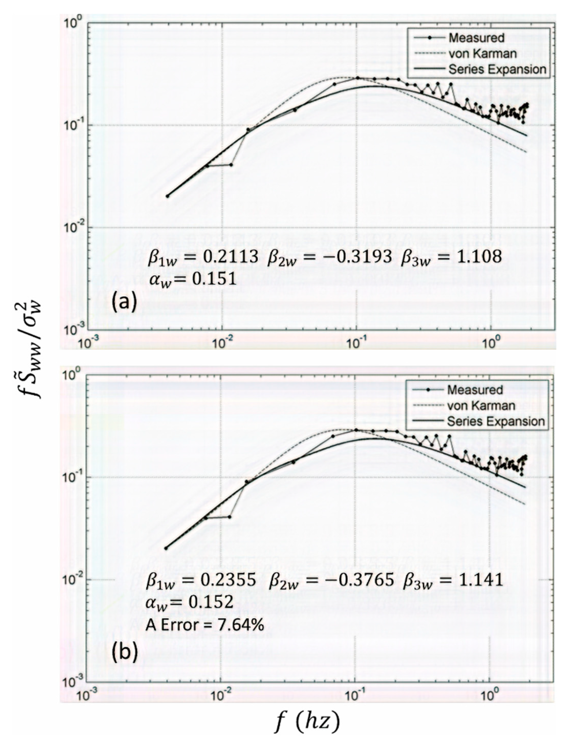These two features, the feasibility of improving the correlation and reducing the “$Aerror$”, is explored in the next figure based on the second-order-correction (a three-term series). The results of Figure 3 are extremely instructive in two respects. First, a comparison of the respective figures (Figure 2a compared to Figure 3a, and Figure 2b compared to Figure 3b) shows that the three-term series model improves the correlation throughout, particularly for $f>{10}^{-1}$ Hz. Second, the “$Aerror$”, which is 23.56% for the two-term series model comes down to 7.64%. Thus, this comparison shows that the three-term series model is a noteworthy improvement over the two-term series model, without or with the enforcement of the −5/3 law. To sum up: modeling based on first-order correction (a two-term series) is generally adequate, and further improvement in correlation and further reduction in “$Aerror=x$” can be achieved through modeling based on second-order correction (a three-term series).

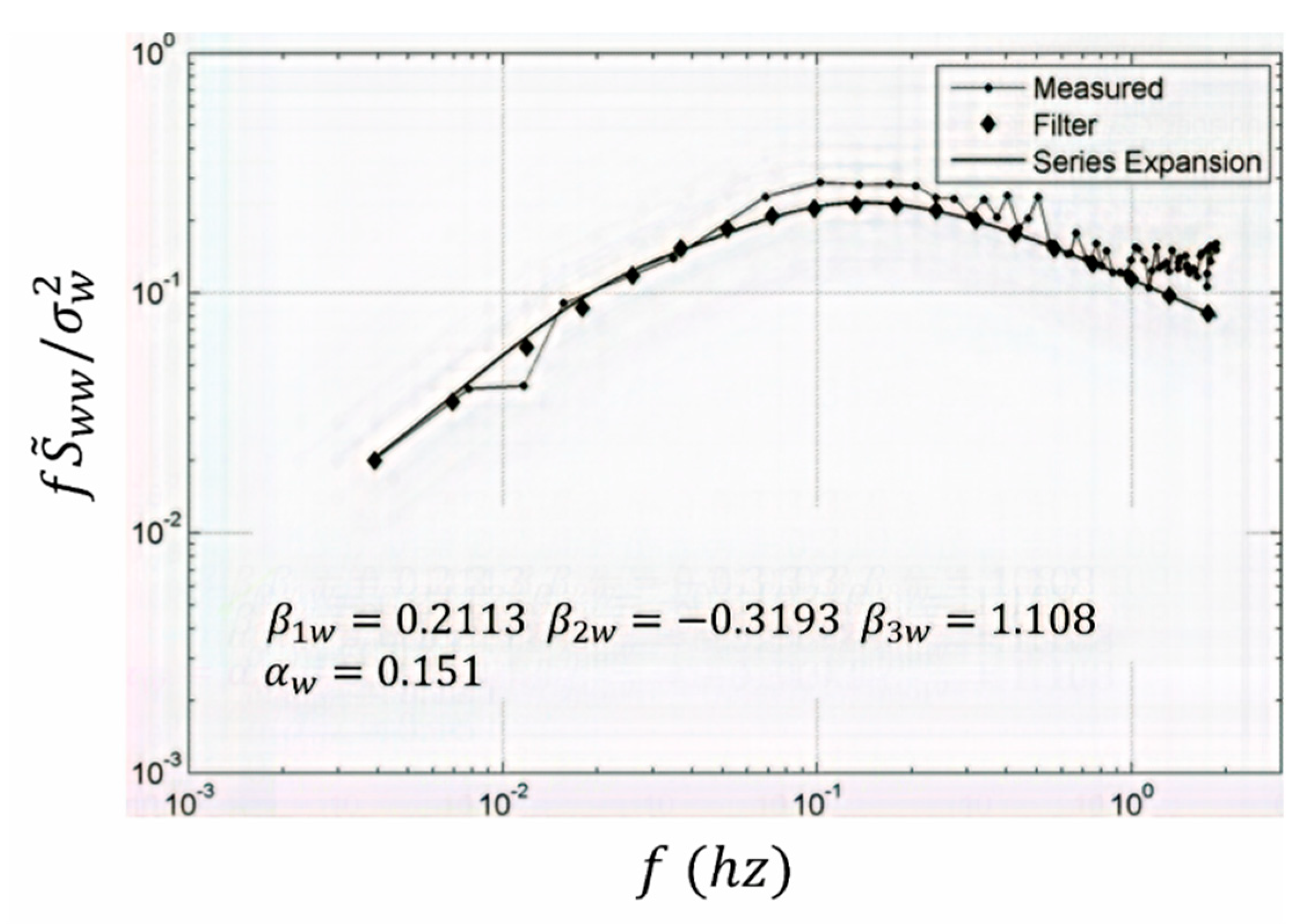
Figure 4 shows how the autospectrum from the white-noise-driven filter for the developed vertical model compares with the one from the database and the developed model itself (specifically, Figure 4 refers to Figure 3a). As seen from this Figure 4, the developed model and simulation are almost indistinguishable. (The filter represents a single-input, single-output system driven by white noise; the design is routine and thus the details are omitted [14]).

5. Methodology of Coherence

As done for autospectra, for coherences also, a mathematical framework is developed for extracting interpretive coherence models from a database of flow velocity points from experimental and CFD investigations. Here as well, each velocity component is considered statistically independent of the other two. For each velocity component, the framework begins with a perturbation series expansion of the coherence; therein, the basis function or the first term of the series is represented by the corresponding coherence for HIT. The perturbation coefficients are evaluated by satisfying the theoretical constraints and fitting a curve on a set of numerically generated coherence points from a database.

In the literature, the development of the cross-spectra and coherences for the longitudinal, vertical and lateral components is scattered and piecemeal; what is more, the expressions for these cross-spectra and coherences show difference among these studies. Accordingly, this section first presents the cross-spectrum, after all, coherence is cross-spectrum that is normalized by the corresponding autospectrum (details to follow). Then it presents the coherences and finally a perturbation theory scheme for the wind-farm wake-turbulence coherence.

5.1. Construction of the Vertical Cross Spectrum

For illustration, vertical turbulence w(t) is considered under headwind conditions. Given $V$, the mean wind velocity, $\tau$, the elapsed time ($t_2-t_1$) and the correlation distance $x=V\tau$, the von Karman correlation function $R_{ww}\left(x\right)$ for vertical turbulence $w\left(t\right)$ is given by Equation (11) [15]:

$$R_{ww}\left(x\right)={\sigma }_w^2\frac{2^{2/3}}{\Gamma \left(1/3\right)}\left[{\left(u\right)}^{1/3}{K}_{1/3}\left(u\right)-\frac{1}{2}{\left(u\right)}^{4/3}{K}_{2/3}\left(u\right)\right]$$

(11)

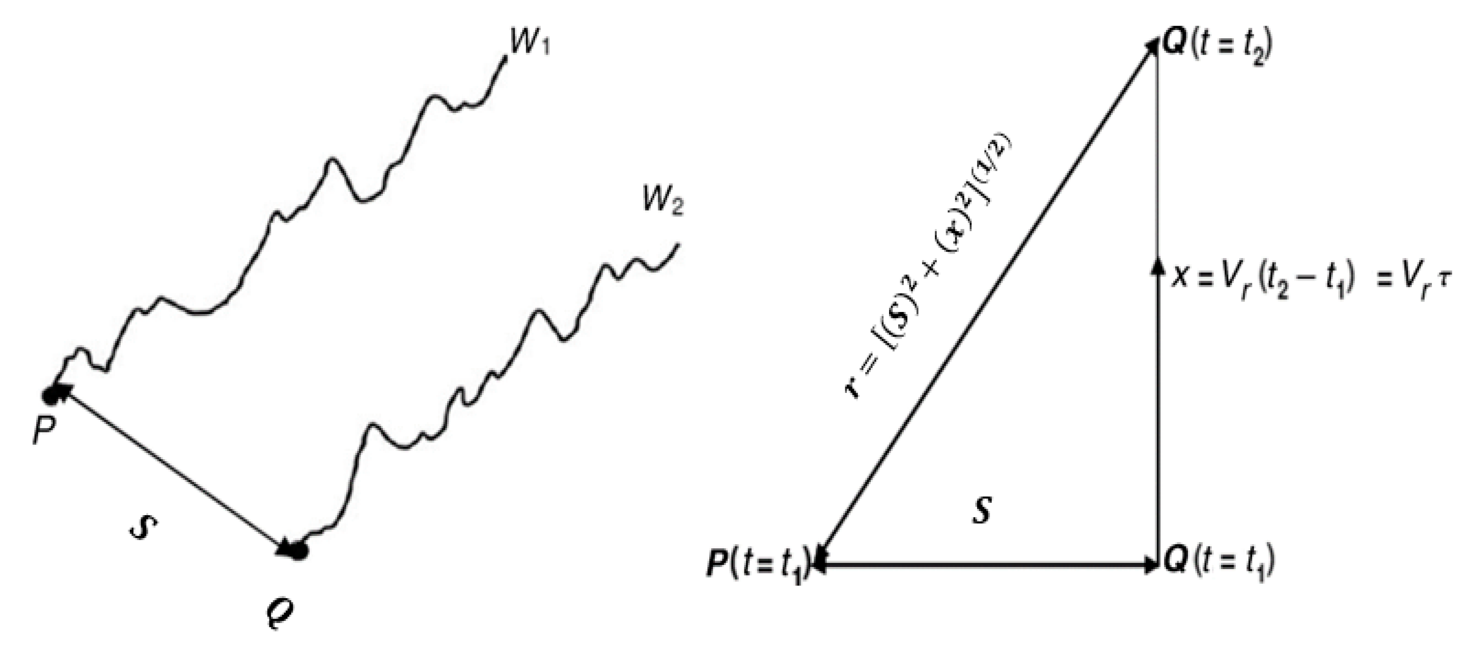
where $u=x$/$1.339L$, $L$ is the scale length and $K_n$ is the modified Bessel function of the second kind. Now consider the cross-correlation between vertical turbulence $w_1\left(t\right)$ at Point 1 and $w_2\left(t\right)$ at Point 2, where these two points are separated by the across-wind distance $S$, as typified by Figure 5. For this scenario, Figure 5 shows that the correlation distance changes to the expression given in Equation (12a):

$$u=\frac{\sigma }{1.339L}\sqrt{1+{\left(\frac{V\tau }{S}\right)}^2}$$

(12a)

where $\sigma =S$/$L$. Now, the cross-correlation $R_{w_1{w}_2}\left(x\right)$ can be expressed as in Equation (12b) [10]:

$$R_{w_1{w}_2}\left(x\right)={\sigma }_w^2\frac{2^{2/3}}{\Gamma \left(1/3\right)}\left[{\left(u\right)}^{1/3}{K}_{1/3}\left(u\right)-\frac{1}{2}{\left(u\right)}^{4/3}{K}_{2/3}\left(u\right)\right]$$

(12b)

The Fourier transform of $R_{w_1{w}_2}\left(\tau \right)$ is the cross-spectrum $S_{w_1{w}_2}\left(\nu \right)$ [10]:

$$S_{w_1{w}_2}\left(\nu \right)={\sigma }_w^2\frac{2^{\frac{2}{3}}}{\Gamma \left(\frac{1}{3}\right)}.\frac{1}{\sqrt{2\pi }}{\left(\frac{1}{1.339}\right)}^{-\frac{8}{3}}\left[\frac{8}{3}{1.339}^2\left(\frac{{\sigma }^{\frac{5}{3}}}{z^{\frac{5}{6}}}\right)K_{\frac{5}{6}}\left(z\right)-\left(\frac{{\sigma }^{\frac{11}{3}}}{z^{\frac{11}{6}}}\right)K_{\frac{11}{6}}\left(z\right)\right]$$

(12c)

where,

$$z=\frac{\sigma }{1.339}\sqrt{1+{\left(1.339\nu \right)}^2}$$

(12d)

In Equation (12d), $\nu$ represents the dimensionless frequency $\nu =\omega L$/$V$ and $\sigma =S$/$L$, the dimensionless distance.

5.2. Coherence for HIT

Coherence is also referred to as spectral correlation coefficient in that it quantifies the normalized cross-correlation between the turbulence velocities at two points as a function of frequency. For illustration, consider the vertical turbulence velocities at two points which are separated by a distance S, as typified by Figure 5. By definition, coherence is given by:

$$C_{w_1{w}_2}\left(\sigma ,\nu \right)=\frac{\left|S_{w_1{w}_2}\left(\nu \right)\right|}{\sqrt{S_{w_1{w}_1}\left(\nu \right)S_{w_2{w}_2}\left(\nu \right)}}$$

(13)

where $S_{w_1{w}_2}\left(\nu \right)$ is the cross-spectrum between vertical turbulence $w_1\left(t\right)$ at Point 1 and $w_2\left(t\right)$ at Point 2, and similarly $S_{w_1{w}_1}\left(\nu \right)$ and $S_{w_2{w}_2}\left(\nu \right)$ are the corresponding autospectra of $w_1\left(t\right)$ and $w_2\left(t\right)$. For HIT, cross-spectrum is real and $S_{w_1{w}_1}\left(\nu \right)\approx S_{w_2{w}_2}\left(\nu \right)$. Therefore, coherence from Equation (13) simplifies to Equation (14).

$$C_{w_1{w}_2}\left(\sigma ,\nu \right)=\frac{\left|S_{w_1{w}_2}\left(\nu \right)\right|}{S_{w_1{w}_1}\left(\nu \right)}$$

(14)

where $S_{w_1{w}_2}\left(\nu \right)$ is given by Equation (12c) and $S_{w_1{w}_1}\left(\nu \right)$ is the von Karman vertical spectrum as given in Equation (15) [15].

$$S_{w_1{w}_1}\left(\nu \right)=\frac{{\sigma }_w^2}{\pi }\left[\frac{1+\frac{8}{3}{\left(1.339\right)}^2}{{\left(1+{1.339}^2\right)}^{11/6}}\right]$$

(15)

As seen from Equation (14), $C_{w_1{w}_2}\left(\sigma ,\nu \right)$ is a ratio of the cross-spectrum from Equation (12c) and the autospectrum from Equation (15). It is expedient to reiterate that this autospectrum is due to von Karman [15] and that the cross-spectrum is due to Houbolt and Sen [10], as an extended version of the von Karman spectral equations that accounts for the cross-correlation between vertical turbulence velocities at two points; also see Figure 5. After some algebra, Equation (14) simplifies to Equation (16) [8].

$$C_{w_1{w}_2}\left(\sigma ,\nu \right)=\frac{0.597}{23869{\left(z/\sigma \right)}^2-1}\left[4.781{\left(z/\sigma \right)}^2{z}^{5/6}{K}_{5/6}\left(z\right)-\frac{1}{2}{z}^{11/6}{K}_{11/6}\left(z\right)\right]$$

(16)

As for the longitudinal and lateral velocity components, the cross-spectra are given by Equations (17a) and (18a) and the coherences are given by Equations (17b) and (18b). In the literature (e.g., [9,10,11,12]), the expressions for cross-spectra and coherences from one set of study do not completely agree from another set.

$$S_{u_1{u}_2}\left(\nu \right)=0.1946{\sigma }_u^2\frac{z^{5/6}}{{\left(1+{\left(1.339\nu \right)}^2\right)}^{11/6}}\left[K_{5/6}\left(z\right)-\frac{z}{2}{K}_{1/6}\left(z\right)\right]$$

(17a)

$$C_{u_1{u}_2}\left(\sigma ,\nu \right)=0.9944z^{5/6}\left[K_{5/6}\left(z\right)-\frac{z}{2}{K}_{1/6}\left(z\right)\right]$$

(17b)

$$S_{v_1{v}_2}\left(\nu \right)=0.0727{\sigma }_v^2\left(\frac{{\sigma }^{5/3}}{z^{5/6}}\right)\left[\frac{8}{3}{K}_{5/6}\left(z\right)-\frac{{\sigma }^2}{{1.339}^{2}z}{K}_{11/6}\left(z\right)+\frac{z}{2}{K}_{1/6}\left(z\right)\right]$$

(18a)

$$C_{v_1{v}_2}\left(\sigma ,\nu \right)=\frac{0.597}{2.8687{\left(z/\sigma \right)}^2-1}\left[4.781{\left(z/\sigma \right)}^2{z}^{5/6}{K}_{5/6}\left(z\right)-\frac{1}{2}{z}^{11/6}{K}_{11/6}\left(z\right)\right]$$

(18b)

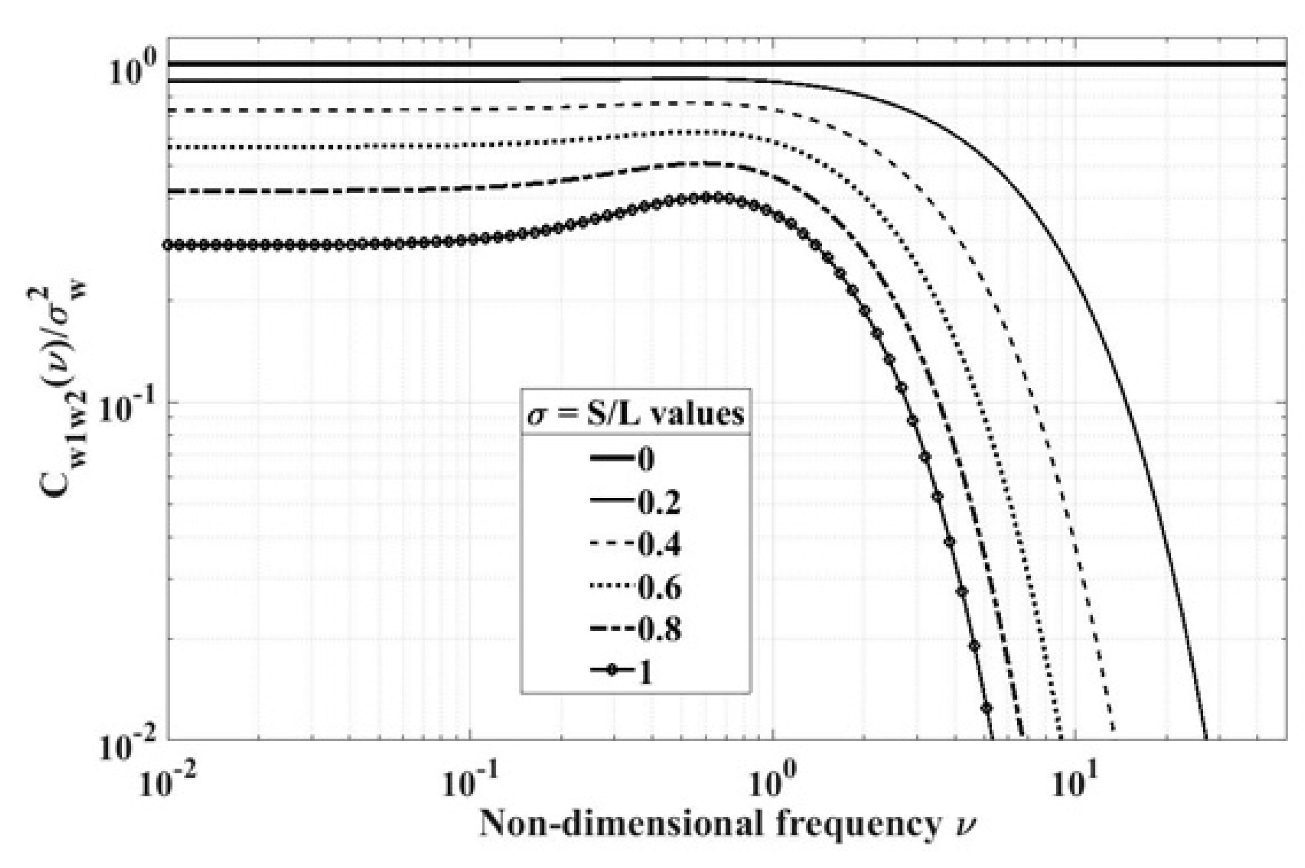
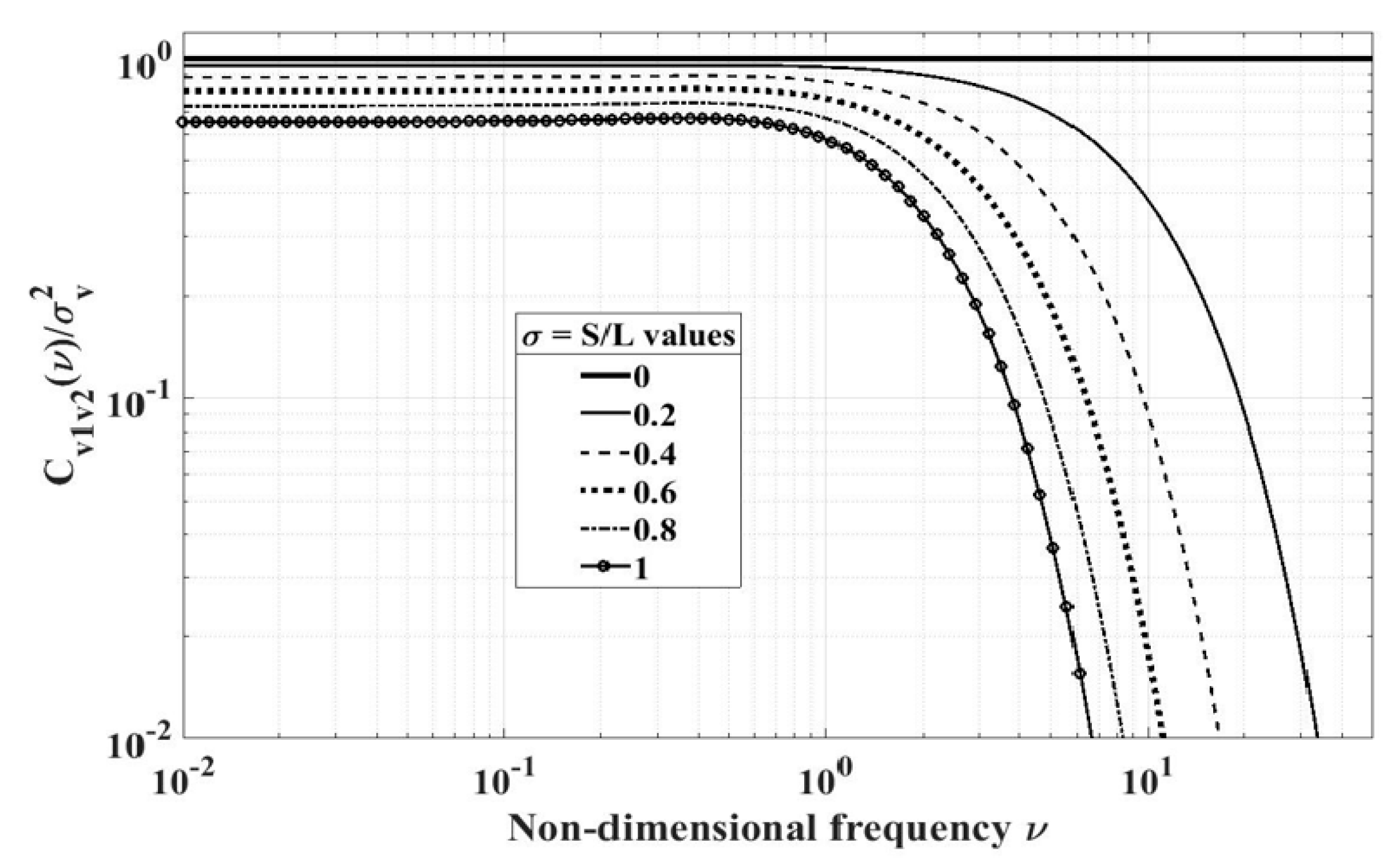
Given this background, it is emphasized that in the present study, the expressions of cross-spectra as typified by Equations (12c), (17a) and (18a) for the vertical, longitudinal and lateral components agree with those of Frost et al. [11]. As for coherence, the corresponding expressions given by Equations (16), (17b) and (18b) agree with those of Irwin [12]. Figure 6, Figure 7 and Figure 8, respectively, show vertical, longitudinal and lateral coherence between Points 1 and 2 as a function of dimensionless frequency $\nu =\omega$L/$V$ for $\sigma =S$/$L=0,0.1,0.2,\dots 1$. For $\sigma =0$, Point 2 merges into Point 1 and in turn the cross-spectra become the respective autospectra and thus the coherence represents the perfect coherence. For example, as seen from Figure 6 for the vertical coherence, $C_{w_1{w}_2}\left(\sigma ,\nu \right)\to 1$. Similarly, as seen from Figure 7 and Figure 8, $C_{u_1{u}_2}\left(\sigma ,\nu \right)\to 1$ and $C_{v_1{v}_2}\left(\sigma ,\nu \right)\to 1$. Exactly the opposite happens with increasing $\sigma$ = S/L. That is, with increasing $\sigma$, the correlation between these two points decreases and so does the corresponding coherence. For example, as seen from Figure 6, Figure 7 and Figure 8, $C_{w_1{w}_2}\left(\sigma ,\nu \right)\to 0$, $C_{u_1{u}_2}\left(\sigma ,\nu \right)\to 0$ and $C_{v_1{v}_2}\left(\sigma ,\nu \right)\to 0$ as $\sigma \to \infty$. Moreover, as seen from these figures, the coherence decreases rapidly for $\nu >1$ or so.

The longitudinal cross-spectrum $S_{u_1{u}_2}\left(\nu \right)$ and coherence $C_{u_1{u}_2}\left(\sigma ,\nu \right)$ are typified by Equations (17a) and (17b), respectively, and Figure 7 shows coherence $C_{u_1{u}_2}\left(\sigma ,\nu \right)$ as a function of dimensionless frequency $\nu =\omega$L/$V$; all of this merits revisiting. The reason is that $S_{u_1{u}_2}\left(\nu \right)$ and in turn the corresponding coherence can become negative at high frequencies. As seen from Equations (17a) and (17b), respectively, $S_{u_1{u}_2}\left(\nu \right)$ and $C_{u_1{u}_2}\left(\sigma ,\nu \right)$ can take on negative values for $K_{5/6}\left(z\right)\le z$/2$K_{1/6}\left(z\right)$. See Figure 9, which is a recasting of Figure 7 for a much expanded vertical scaling (1 to ${10}^{-6}$ in Figure 9 in comparison to 1 to ${10}^{-2}$ in Figure 7). The crosses (*) in Figure 9 indicate the termination of the curve to avoid generating negative coherence values. Given the state of the art and one’s initiation into cross-spectra and coherence, it is difficult to come up with a basis for these negative values of cross-spectrum and coherence for HIT; a resolution of this difficulty would require further research [11].

5.3. Coherence Modeling for Wind-Farm Wake Turbulence

Wind farm wake turbulence deviates from HIT. Accordingly, the framework for coherence modeling from a database accounts for this deviation based on perturbation theory. Here as well, the framework assumes the same topology that was assumed in the development of the basis functions; for illustration vertical coherence $C_{w_1{w}_2}\left(\sigma ,\nu \right)$ is selected.

Let $C_{w_1{w}_2}\left(\sigma ,\nu \right)$ represent the vertical coherence of wake turbulence. The framework begins with a perturbation series expansion of ${\tilde{C}}_{w_1{w}_2}\left(\sigma ,\nu \right)$ (essentially the same procedure applies to the other two components):

$${\tilde{C}}_{w_1{w}_2}\left(\sigma ,\nu \right)=C_{1w}{C}_{w_1{w}_2}\left(\sigma ,\nu \right)+C_{2w}{C}_{w_1{w}_2}^2\left(\sigma ,\nu \right)+\cdots +C_{nw}{C}_{w_1{w}_2}^n\left(\sigma ,\nu \right)$$

(19)

The basis function or the first term of the series is given by Equation (16). Since $C_{w_1{w}_2}\left(\sigma ,\nu \right)=1$ for $\sigma =0$, Equation (17) is subject to the constraint:

$$C_{1w}+C_{2w}+\cdots +C_{nw}=1$$

(20)

The second condition that ${\tilde{C}}_{w_1{w}_2}\left(\sigma ,\nu \right)=0$ for $\sigma =\infty$ is automatically satisfied since $C_{w_1{w}_2}\left(\sigma ,\nu \right)=0$ for $\sigma =\infty$. The coefficients in the series $C_{iw}$ are evaluated by satisfying the theoretical constraint of Equation (20) and fitting a curve on a set of selected numerically generated coherence points in a least squares sense.

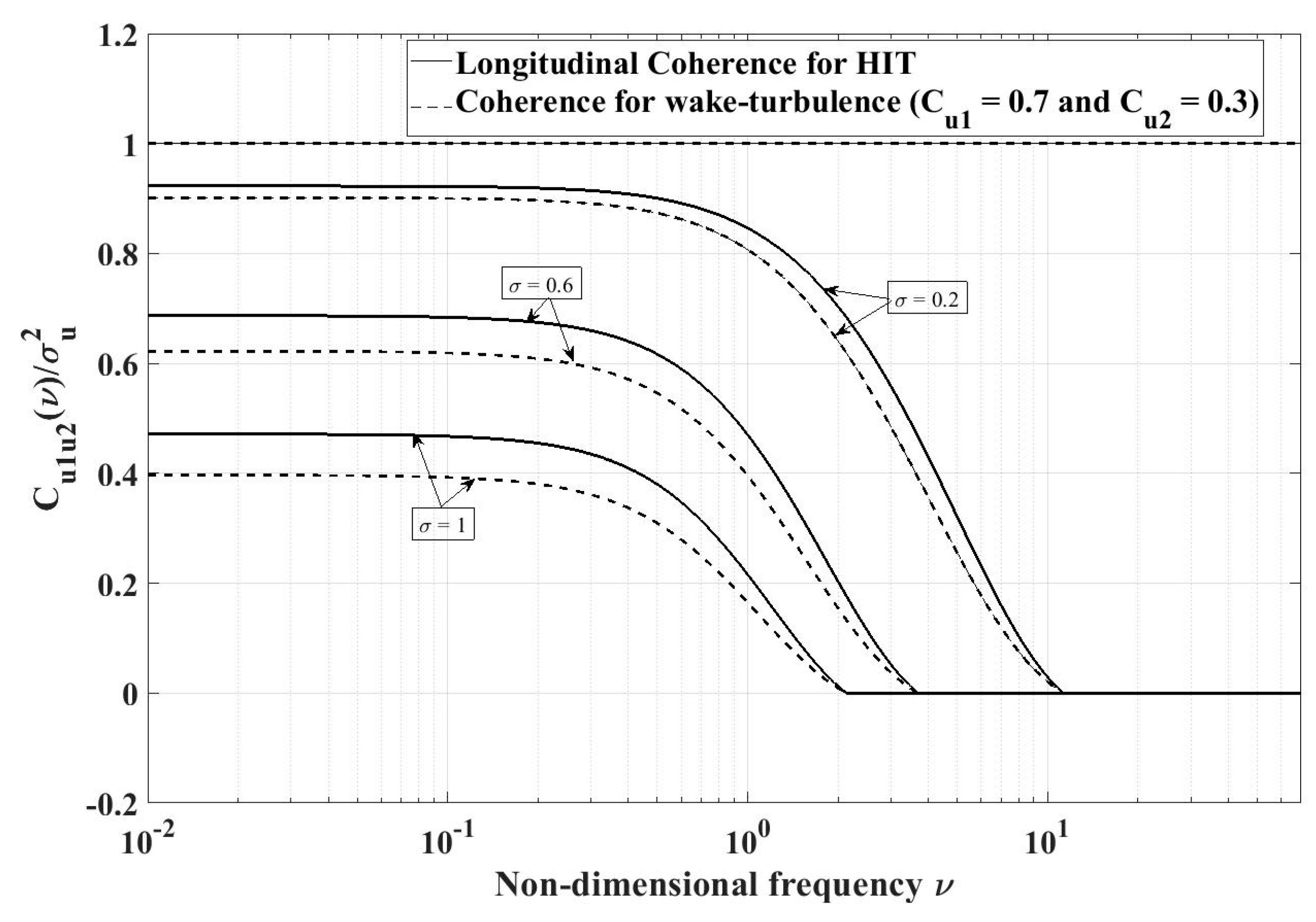
For illustrations, longitudinal coherence of wake turbulence ${\tilde{C}}_{u_1{u}_2}\left(\sigma ,\nu \right)$ is selected with a two- term perturbation series (also see Equation (19)):

$${\tilde{C}}_{u_1{u}_2}\left(\sigma ,\nu \right)=C_{1u}{C}_{u_1{u}_2}\left(\sigma ,\nu \right)+C_{2u}{C}_{u_1{u}_2}^2\left(\sigma ,\nu \right)$$

(21)

Specifically, consider $C_{1u}=0.7$ and $C_{2u}=0.3$ (also see constraint Equation (20)). Descriptively stated, this case represents wake turbulence, which deviates weakly from HIT. It is plausible that this case belongs to wake turbulence at locations that are downwind of the first two rows or so. Therein, wake turbulence is expected to deviate only weakly from HIT as depicted in Figure 10.

6. Conclusions

This study has shown that an earlier-exercised mathematical framework lends itself well to extracting interpretive autospectral models of wind farm wake turbulence from a database. While these models are database specific, the framework can be applied to any database and the model construction is straightforward. As to the two-point statistics of wake-turbulence, this study first presents a unified account of cross-spectrum and coherence for HIT; this account is of considerable utility in that, in the literature, the expressions of cross-spectrum and coherence show differences from one study to the other. Given these expressions of coherences, this study then builds a framework for extracting wake turbulence coherence models from a database. The frameworks for autospectra and coherences do not follow classical perturbation theory approach of a solution for a linearized problem along with successively added corrections. Both frameworks represent a practical combination of a series expansion, exploitation of a database, and theoretical constraints in closed form.

This study also leads to following specific findings:

• Generally, no more than a three-term series (second-order correction) is necessary to develop an autospectral model; in most cases, a two-term series (first-order correction) is found to be adequate for wind engineering applications.
• The addition of a third term to the series has significant power in reducing the “$Aerror$” between the model and the data. Recall that the “$Aerror$” refers to minimizing the sum of the errors in a least squares sense: the model deviation from the autospectral data points and from the measured high frequency autospectral decay level (when applicable).
• These developed models lend themselves well to design of filters driven by white noise; that is, the filter design is as routine as the currently used procedure for the von Kármán models.
• While this framework to constructing the coherence models from a database has not been tested against a database, it has been formulated from first principles and with a theoretical basis.
• This study has shown the feasibility of constructing both the one-point statistics of autospectral models and the two-point statistics of coherence models from a database. These models could serve as surrogate analytical models in the experimental and CFD investigations; thus, this feasibility offers promise in providing an improved understanding of wake turbulence.
• The two frameworks for the autospectrum and coherence increase the utility base of the database, involving enormous resources. Given the simple analytical structure of these models, they bring better understanding and transparency to a dataset.