An Improved LSSVM Model for Intelligent Prediction of the Daily Water Level


Abstract
1. Introduction
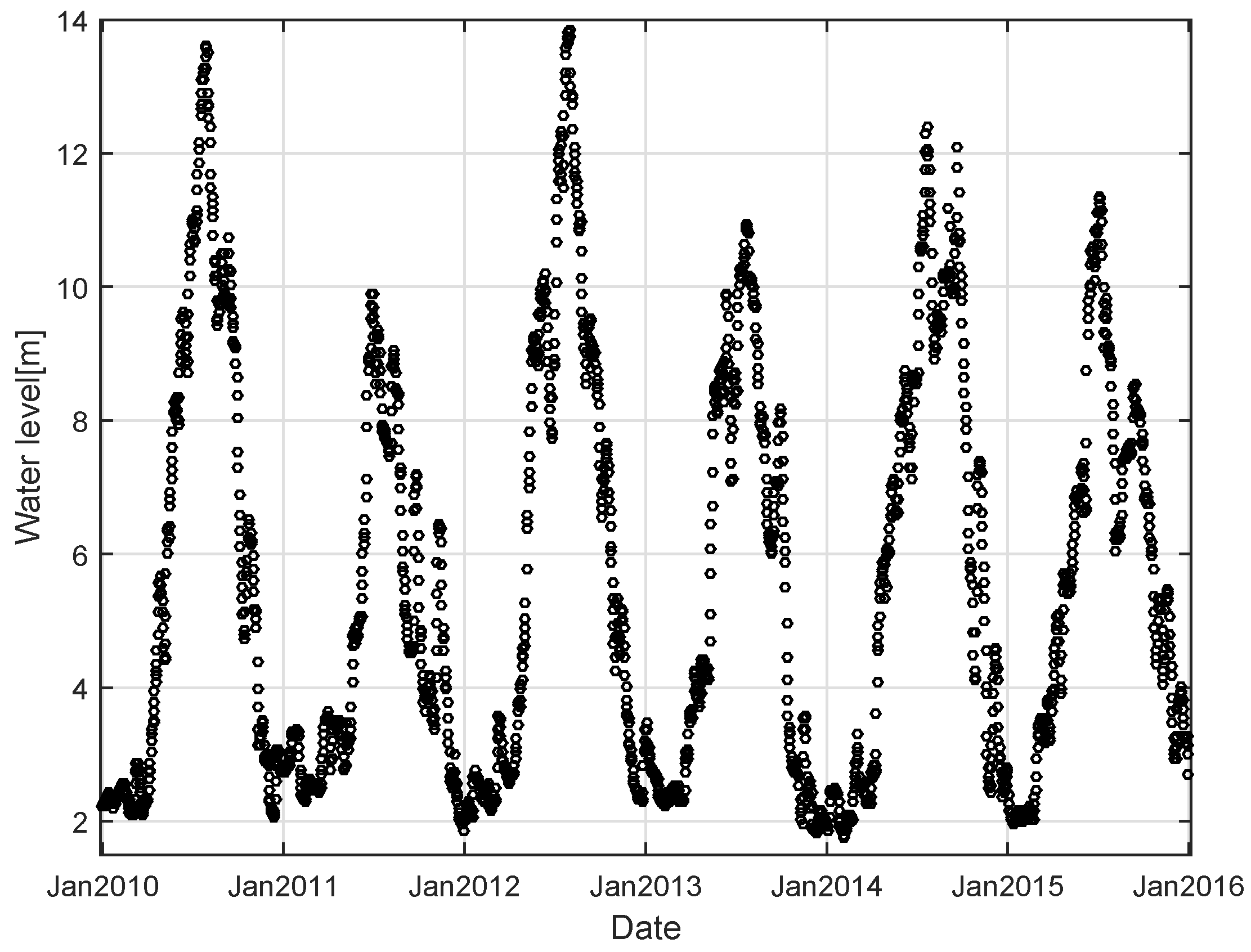
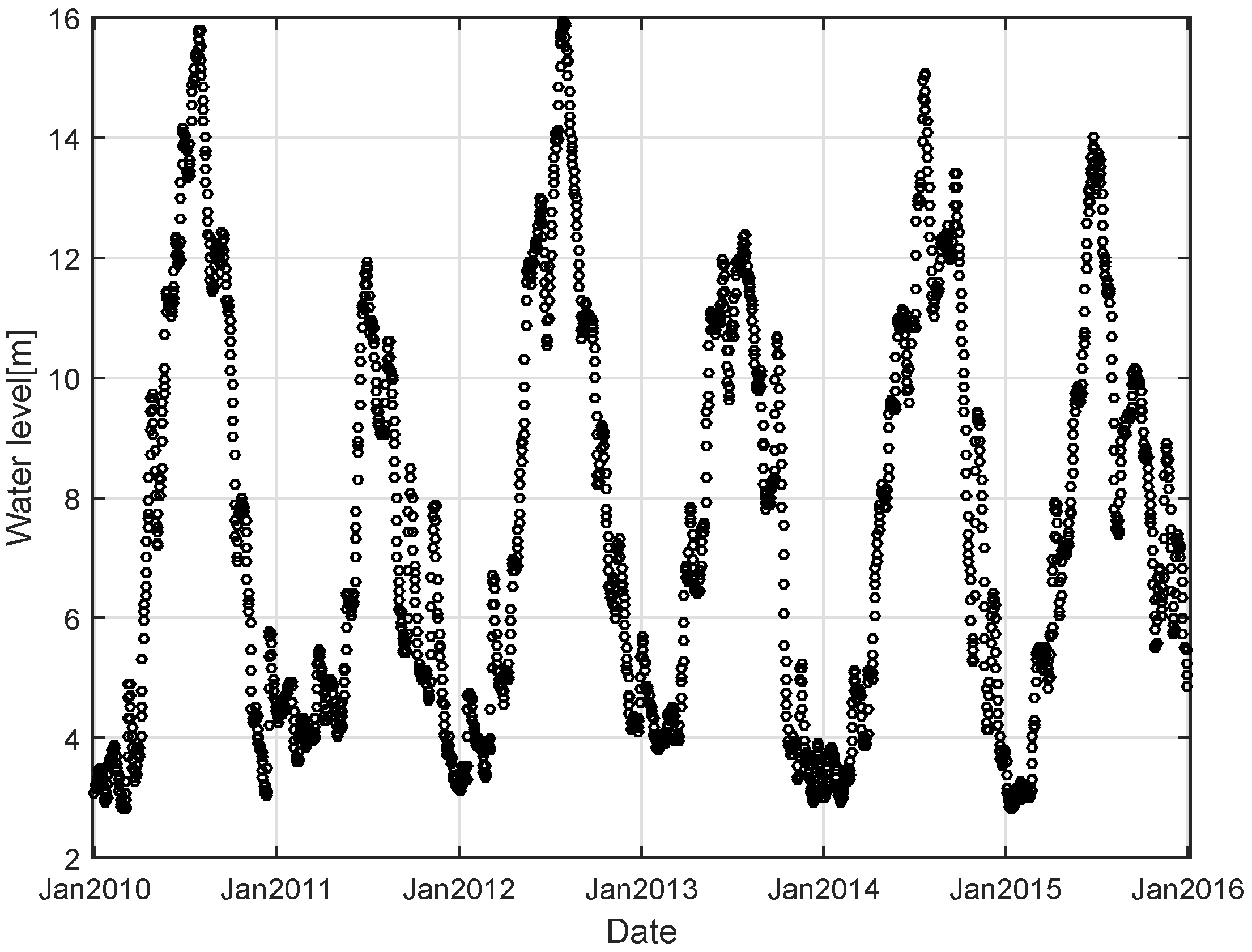
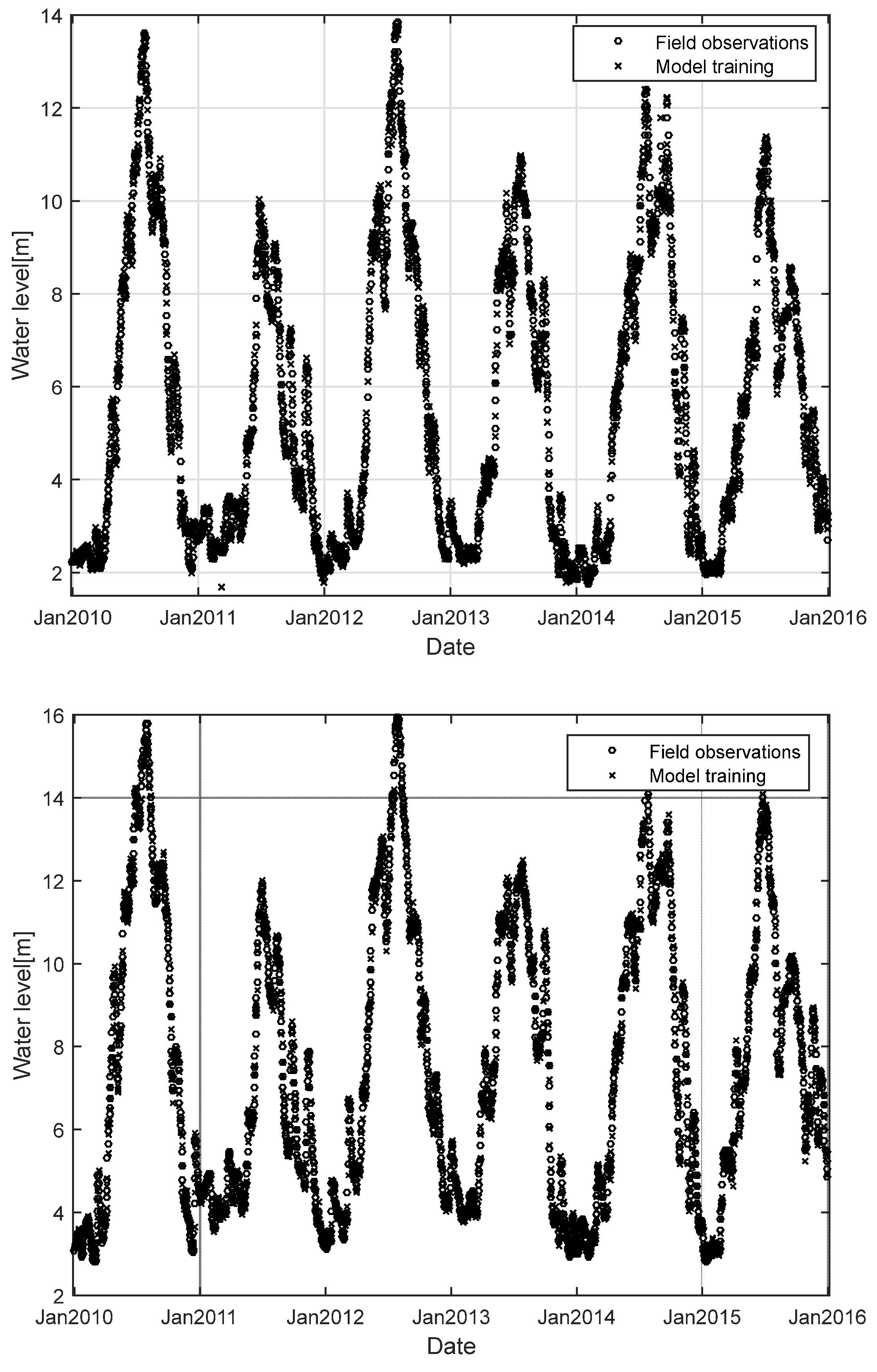
2. Data Source
3. Methodology
3.1. Conventional LSSVM Model
3.2. Improved LSSVM Model
3.3. Model Performace Metrics
4. Result and Discussion
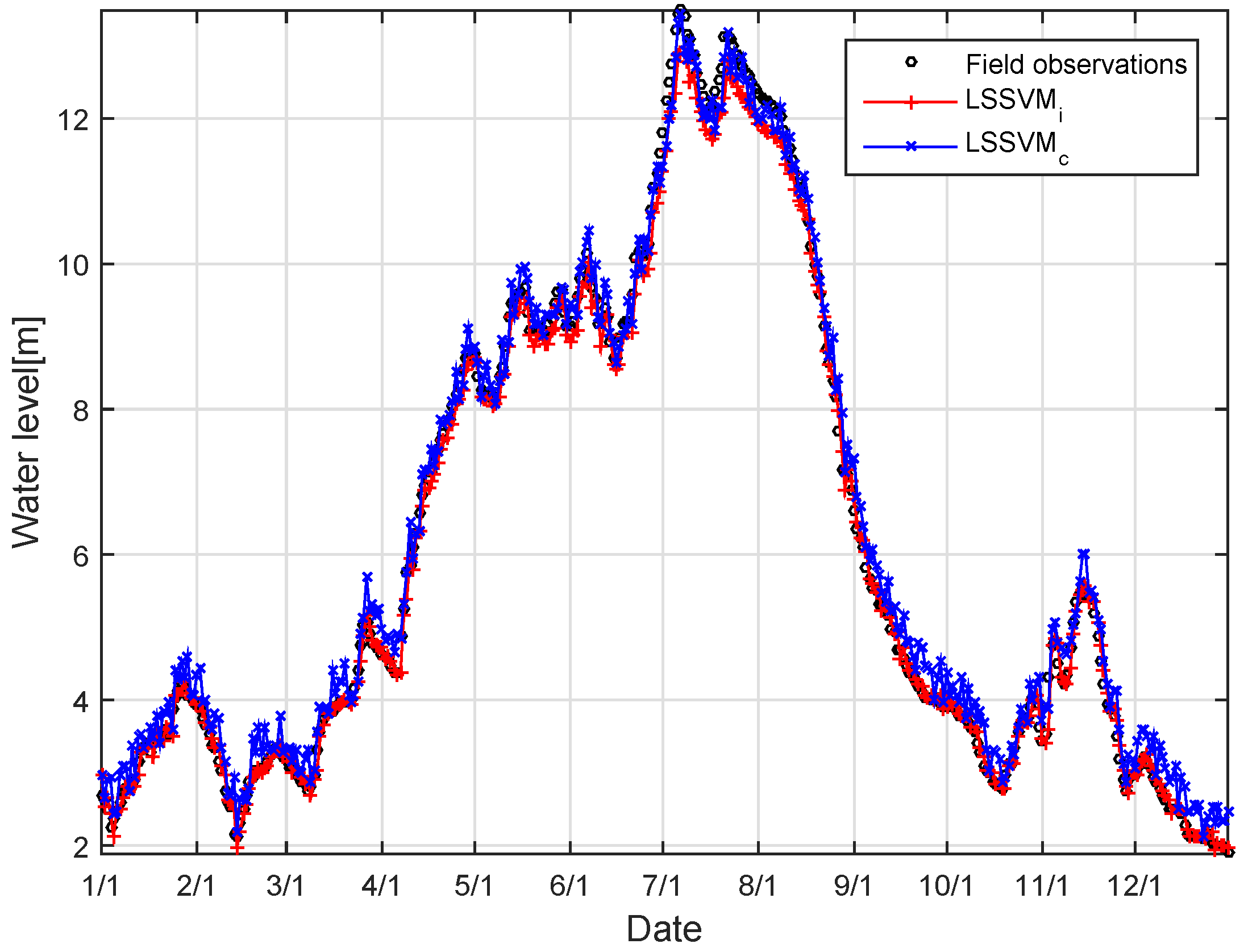
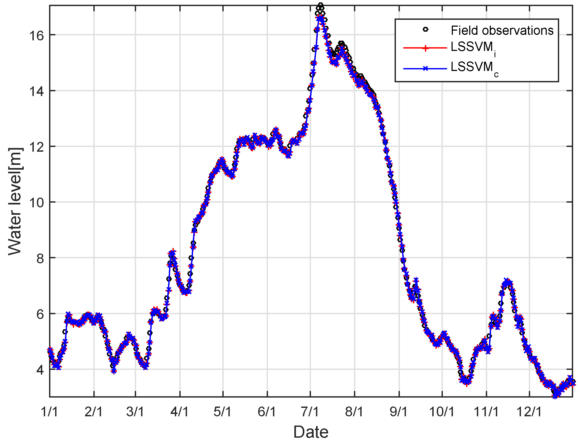
4.1. LSSVMi Forecasting of Daily Water Level
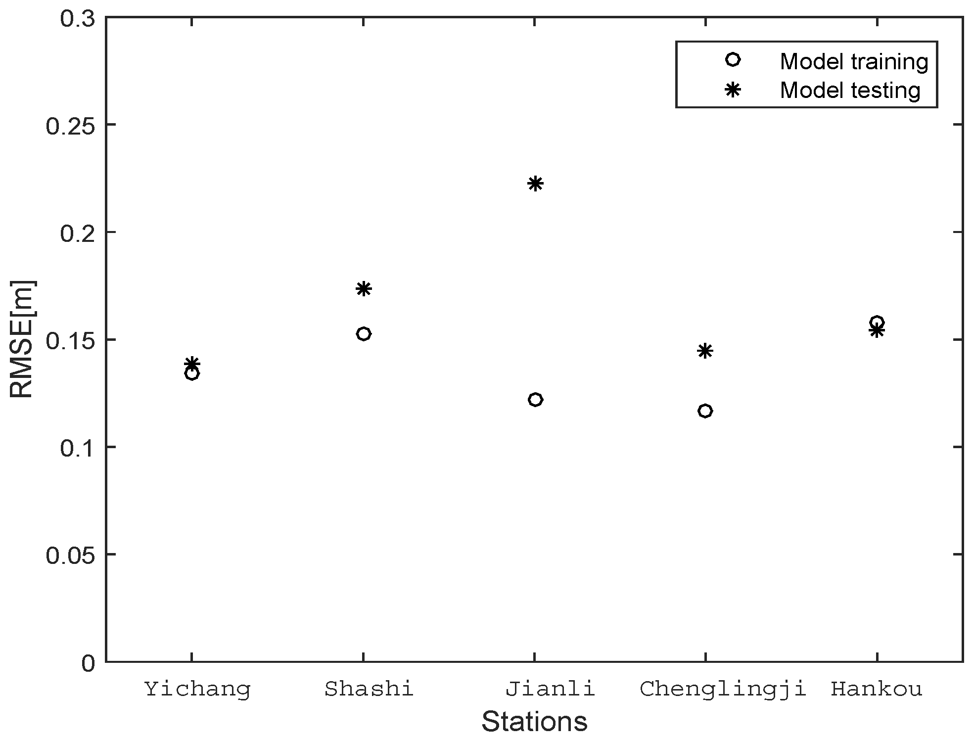
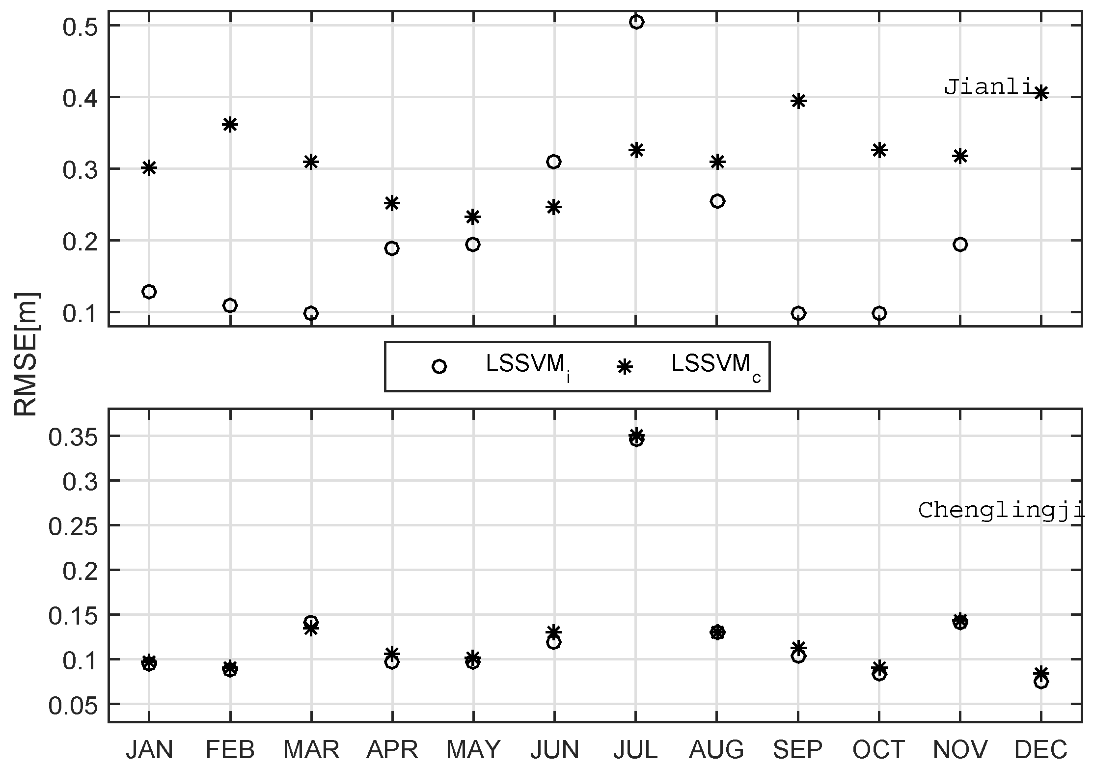
4.2. Model Performance Evaluation
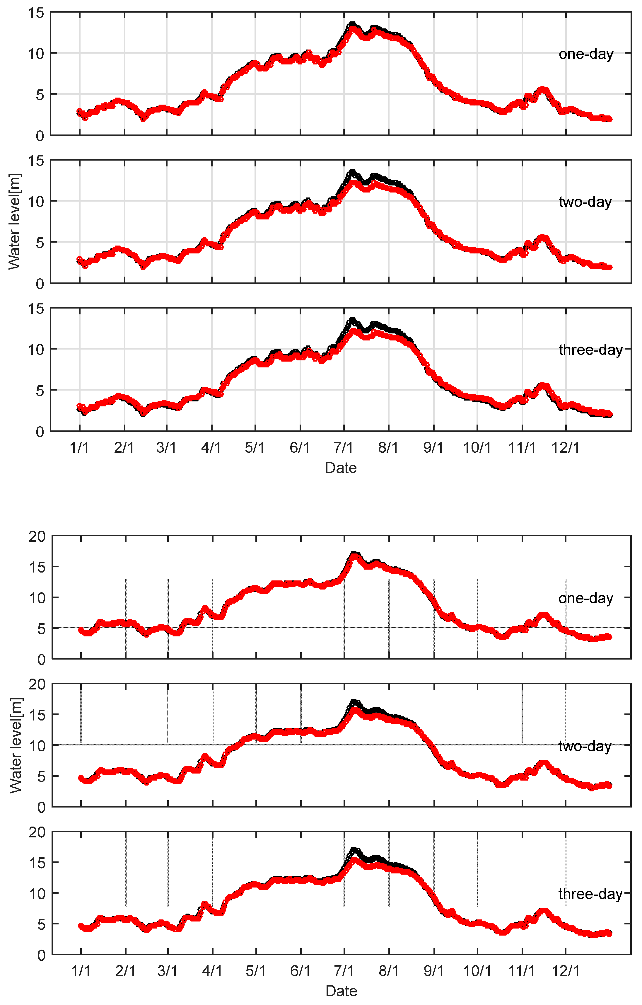
4.3. Influence of Forecast Lead Time
5. Conclusions
Author Contributions
Funding
Acknowledgments
Conflicts of Interest
References
- Choi, K.H.; Ang, B.W. A time-series analysis of energy-related carbon emissions in Korea. Energy Policy 2001, 29, 1155–1161. [Google Scholar] [CrossRef]
- Montoya, J.V.; Roelke, D.L.; Winemiller, K.O.; Cotner, J.B.; Snider, J.A. Hydrological seasonality and benthic algal biomass in a Neotropical floodplain river. J. N. Am. Benthol. Soc. 2006, 25, 157–170. [Google Scholar] [CrossRef]
- Buyukyildiz, M.; Tezel, G.; Yilmaz, V. Estimation of the Change in Lake Water Level by Artificial Intelligence Methods. Water Resour. Manag. 2014, 28, 4747–4763. [Google Scholar] [CrossRef]
- Kisi, O.; Shiri, J.; Nikoofar, B. Forecasting daily lake levels using artificial intelligence approaches. Comput. Geosci. 2012, 41, 169–180. [Google Scholar] [CrossRef]
- Sulaiman, M.; El-Shafie, A.; Karim, O.; Basri, H. Improved Water Level Forecasting Performance by Using Optimal Steepness Coefficients in an Artificial Neural Network. Water Resour. Manag. 2011, 25, 2525–2541. [Google Scholar] [CrossRef]
- Zhong, C.; Jiang, Z.; Chu, X.; Guo, T.; Wen, Q. Water level forecasting using a hybrid algorithm of artificial neural networks and local Kalman filtering. Proc. Inst. Mech. Eng. Part M J. Eng. Marit. Environ. 2017. [Google Scholar] [CrossRef]
- Alvisi, S.; Mascellani, G.; Franchini, M.; Bardossy, A. Water level forecasting through fuzzy logic and artificial neural network approaches. Hydrol. Earth Syst. Sci. Discuss. 2005, 2, 1107–1145. [Google Scholar] [CrossRef]
- Palani, S.; Liong, S.Y.; Tkalich, P. An ANN application for water quality forecasting. Mar. Pollut. Bull. 2008, 56, 1586–1597. [Google Scholar] [CrossRef]
- Nourani, V.; Mogaddam, A.A.; Nadiri, A.O. An ANN-based model for spatiotemporal groundwater level forecasting. Hydrol. Process. 2010, 22, 5054–5066. [Google Scholar] [CrossRef]
- Ivan, H.; Gilja, G. Time series forecasting of parameters in hydraulic engineering using artificial neural networks. In Proceedings of the International Symposium on Water Management & Hydraulic Engineering, Primošten, Hrvatska, 6–8 September 2017. [Google Scholar]
- Valizadeh, N.; El-Shafie, A.; Mirzaei, M.; Galavi, H.; Mukhlisin, M.; Jaafar, O. Accuracy Enhancement for Forecasting Water Levels of Reservoirs and River Streams Using a Multiple-Input-Pattern Fuzzification Approach. Sci. World J. 2014, 2014, 432976. [Google Scholar] [CrossRef] [PubMed]
- Kang, M.G.; Maeng, S.J. Gray Models for Real-Time Groundwater-Level Forecasting in Irrigated Paddy-Field Districts. J. Irrig. Drain. Eng. 2015, 142, 04015036. [Google Scholar] [CrossRef]
- Guo, Z.; Bai, G. Application of Least Squares Support Vector Machine for Regression to Reliability Analysis. Chin. J. Aeronaut. 2009, 22, 160–166. [Google Scholar] [CrossRef]
- Luo, W.L.; Zou, Z.J. Parametric Identification of Ship Maneuvering Models by Using Support Vector Machines. J. Ship Res. 2009, 53, 19–30. [Google Scholar]
- Sujay Raghavendra, N.; Deka, P.C.; Shukla, S. Forecasting monthly groundwater level fluctuations in coastal aquifers using hybrid Wavelet packet–Support vector regression. Cogent Eng. 2015, 2, 999414. [Google Scholar] [CrossRef]
- Seo, Y.; Kim, S.; Singh, V.P. Physical Interpretation of River Stage Forecasting Using Soft Computing and Optimization Algorithms. In Harmony Search Algorithm; Springer: Berlin/Heidelberg, Germany, 2016. [Google Scholar]
- Francesco, G.; Rudy, G.; Giovanni, D.M. Support Vector Regression for Rainfall-Runoff Modeling in Urban Drainage: A Comparison with the EPA’s Storm Water Management Model. Water 2016, 8, 69. [Google Scholar] [CrossRef]
- Noori, R.; Karbassi, A.R.; Moghaddamnia, A.; Han, D.; Zokaei-Ashtiani, M.H.; Farokhnia, A.; Gousheh, M.G. Assessment of input variables determination on the SVM model performance using PCA, Gamma test, and forward selection techniques for monthly stream flow prediction. J. Hydrol. (Amst.) 2011, 401, 177–189. [Google Scholar] [CrossRef]
- Kisi, O.; Cimen, M. Precipitation forecasting by using wavelet-support vector machine conjunction model. Eng. Appl. Artif. Intell. 2012, 25, 783–792. [Google Scholar] [CrossRef]
- Cheng, M.Y.; Hoang, N.D.; Wu, Y.W. Cash flow prediction for construction project using a novel adaptive time-dependent least squares support vector machine inference model. J. Civ. Eng. Manag. 2015, 21, 679–688. [Google Scholar] [CrossRef]
- Cong, Y.; Wang, J.; Li, X. Traffic Flow Forecasting by a Least Squares Support Vector Machine with a Fruit Fly Optimization Algorithm. Procedia Eng. 2016, 137, 59–68. [Google Scholar] [CrossRef]
- Ismail, S.; Shabri, A.; Samsudin, R. A hybrid model of self-organizing maps (SOM) and least square support vector machine (LSSVM) for time-series forecasting. Expert Syst. Appl. 2011, 38, 10574–10578. [Google Scholar] [CrossRef]
- Li, S.; Xiong, L.; Dong, L.; Zhang, J. Effects of the Three Gorges Reservoir on the hydrological droughts at the downstream Yichang station during 2003–2011. Hydrol. Process. 2013, 27, 3981–3993. [Google Scholar] [CrossRef]
- Guo, J.; Zhou, J.; Qin, H.; Zou, Q.; Li, Q. Monthly streamflow forecasting based on improved support vector machine model. Expert Syst. Appl. 2011, 38, 13073–13081. [Google Scholar] [CrossRef]
- Ghorbani, M.A.; Khatibi, R.; Goel, A.; FazeliFard, M.H.; Azani, A. Modeling river discharge time series using support vector machine and artificial neural networks. Environ. Earth Sci. 2016, 75, 685. [Google Scholar] [CrossRef]
- Willmott, C. On the validation of models. Phys. Geogr. 1981, 2, 184–194. [Google Scholar] [CrossRef]


| Lead Time | Parameter | Yichang | Shashi | Jianli | Chenglingji | Hankou |
|---|---|---|---|---|---|---|
| 1-day | 6.655e7 | 5.488e8 | 7.59e8 | 8.43e7 | 8.41e8 | |
| 1.75e6 | 3.489e2 | 2.688e7 | 6.93e2 | 4.85e3 | ||
| 2-day | 6.555e7 | 5.889e9 | 6.95e8 | 8.43e7 | 8.43e8 | |
| 2.75e6 | 3.689e2 | 1.388e7 | 5.99e2 | 2.97e5 | ||
| 3-day | 6.455e7 | 5.889e6 | 6.59e8 | 8.43e7 | 7.41e9 | |
| 3.75e6 | 1.789e3 | 1.188e7 | 5.95e3 | 3.07e5 |
| Stations | RMSE [m] | MAPE [%] [-] | D [-] | |||
|---|---|---|---|---|---|---|
| LSSVMc | LSSVMi | LSSVMc | LSSVMi | LSSVMc | LSSVMi | |
| Yichang | 0.1394 | 0.1384 | 10.0872 | 8.6710 | 0.9848 | 0.9863 |
| Shashi | 0.1727 | 0.1740 | 20.7350 | 20.5456 | 0.9796 | 0.9794 |
| Jianli | 0.3196 | 0.2222 | 6.1984 | 2.4874 | 0.9552 | 0.9736 |
| Chenglingji | 0.1482 | 0.1449 | 1.3801 | 1.3232 | 0.9852 | 0.9857 |
| Hankou | 0.1536 | 0.1546 | 1.5315 | 1.4613 | 0.9862 | 0.9865 |
| Stations | Yichang | Shashi | Jianli | Chenglingji | Hankou |
|---|---|---|---|---|---|
| LSSVMi | 0.9726 | 0.9235 | 1.0000 | 1.0000 | 1.0000 |
| LSSVMc | 0.9671 | 0.9207 | 0.9644 | 1.0000 | 1.0000 |
| Stations | RMSE [m] | MAPE [%] | D [-] | ||||||
|---|---|---|---|---|---|---|---|---|---|
| 1-day | 2-day | 3-day | 1-day | 2-day | 3-day | 1-day | 2-day | 3-day | |
| Jianli | 0.2222 | 0.3755 | 0.4175 | 2.4874 | 3.1273 | 4.7808 | 0.9736 | 0.9603 | 0.9489 |
| Chenglingji | 0.1448 | 0.3262 | 0.4056 | 1.3232 | 1.9215 | 2.1845 | 0.9857 | 0.9737 | 0.9681 |
© 2018 by the authors. Licensee MDPI, Basel, Switzerland. This article is an open access article distributed under the terms and conditions of the Creative Commons Attribution (CC BY) license (http://creativecommons.org/licenses/by/4.0/).
Share and Cite
Guo, T.; He, W.; Jiang, Z.; Chu, X.; Malekian, R.; Li, Z. An Improved LSSVM Model for Intelligent Prediction of the Daily Water Level. Energies 2019, 12, 112. https://doi.org/10.3390/en12010112
Guo T, He W, Jiang Z, Chu X, Malekian R, Li Z. An Improved LSSVM Model for Intelligent Prediction of the Daily Water Level. Energies. 2019; 12(1):112. https://doi.org/10.3390/en12010112
Chicago/Turabian StyleGuo, Tao, Wei He, Zhonglian Jiang, Xiumin Chu, Reza Malekian, and Zhixiong Li. 2019. "An Improved LSSVM Model for Intelligent Prediction of the Daily Water Level" Energies 12, no. 1: 112. https://doi.org/10.3390/en12010112
APA StyleGuo, T., He, W., Jiang, Z., Chu, X., Malekian, R., & Li, Z. (2019). An Improved LSSVM Model for Intelligent Prediction of the Daily Water Level. Energies, 12(1), 112. https://doi.org/10.3390/en12010112