Figure 1.
The flowchart of the constriction factor particle swarm optimization.
Figure 1.
The flowchart of the constriction factor particle swarm optimization.
Figure 2.
Fault location/faulty section identification flowchart employing the ST based MLT approach.
Figure 2.
Fault location/faulty section identification flowchart employing the ST based MLT approach.
Figure 3.
Four-node test distribution feeder used for fault location purpose.
Figure 3.
Four-node test distribution feeder used for fault location purpose.
Figure 4.
Comparison of the Stockwell transform (ST) based non-optimized MLT predicted and actual fault distances, for the test dataset of applied phase-A-to-ground (AG) fault.
Figure 4.
Comparison of the Stockwell transform (ST) based non-optimized MLT predicted and actual fault distances, for the test dataset of applied phase-A-to-ground (AG) fault.
Figure 5.
Scatter plot of the targeted and the ST based non-optimized MLT predicted outputs, for the test dataset of AG fault.
Figure 5.
Scatter plot of the targeted and the ST based non-optimized MLT predicted outputs, for the test dataset of AG fault.
Figure 6.
Comparison of the ST based constriction factor-based particle swarm optimization (CF-PSO) optimized MLT predicted and actual fault distances for the test dataset of AG fault.
Figure 6.
Comparison of the ST based constriction factor-based particle swarm optimization (CF-PSO) optimized MLT predicted and actual fault distances for the test dataset of AG fault.
Figure 7.
Scatter plot of the targeted and the ST based CF-PSO optimized MLT predicted outputs for the test dataset of AG fault.
Figure 7.
Scatter plot of the targeted and the ST based CF-PSO optimized MLT predicted outputs for the test dataset of AG fault.
Figure 8.
Comparison of the ST based optimized MLT predicted and actual fault distances, for the test dataset, in the presence of 30 dB SNR.
Figure 8.
Comparison of the ST based optimized MLT predicted and actual fault distances, for the test dataset, in the presence of 30 dB SNR.
Figure 9.
Scatter plot of the targeted and the ST based optimized MLT predicted outputs, for the test dataset, in the presence of 30 dB SNR.
Figure 9.
Scatter plot of the targeted and the ST based optimized MLT predicted outputs, for the test dataset, in the presence of 30 dB SNR.
Figure 10.
Comparison of the ST based optimized MLT predicted and actual fault distances, for the test dataset, in the presence of 20 dB SNR.
Figure 10.
Comparison of the ST based optimized MLT predicted and actual fault distances, for the test dataset, in the presence of 20 dB SNR.
Figure 11.
Scatter plot of the targeted and the ST based optimized MLT predicted outputs, for the test dataset, in the presence of 20 dB SNR.
Figure 11.
Scatter plot of the targeted and the ST based optimized MLT predicted outputs, for the test dataset, in the presence of 20 dB SNR.
Figure 12.
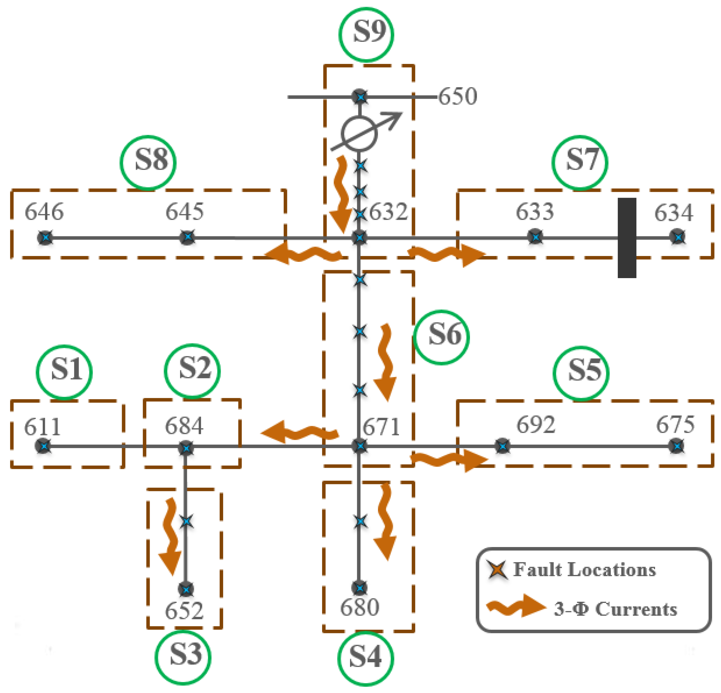
IEEE thirteen-node test distribution feeder.
Figure 12.
IEEE thirteen-node test distribution feeder.
Table 1.
ST Extracted Feature Selection and Removal Process Summary.
Table 1.
ST Extracted Feature Selection and Removal Process Summary.
| Selected Features | Correlation Factor/Comment | Action |
|---|
| F5 & F6 | 1.00 | Remove feature F6 |
| F9 & F13 | 1.00 | Remove feature F13 |
| F21 & F24 | 1.00 | Remove feature F24 |
| F25 & F28 | 1.00 | Remove feature F28 |
| F21 & F25 | 0.9999 | Remove feature F25 |
| F5 & F9 | 0.9997 | Remove feature F9 |
| F11 & F15 | 0.9996 | Remove feature F15 |
| F5 & F8 | 0.9965 | Remove feature F8 |
| F22 & F26 | 0.9958 | Remove feature F26 |
| F7 & F11 | 0.9957 | Remove feature F7 |
| F8, F12 & F16 | 1.00 | Remove features F12 & F16 |
| F17, F19 & F20 | Most of the cases they are zero | Remove all of them |
| F27 | It is constant for all cases | Remove F27 |
| The selected features: F1, F2, F3, F4, F5, F10, F11, F14, F18, F21, F22, and F23 |
Table 2.
Four-node test distribution feeder specifications.
Table 2.
Four-node test distribution feeder specifications.
| Item | Details |
|---|
| Transformer I | 12 MVA, 120/25 kV, Yg-D |
| Transformer II | 12 MVA, 25 kV/575 V, Yg-D |
| Length of distribution line | 30 km |
| System frequency | 60 Hz |
| Load (Unbalanced) | Phase A (1 MW, 0.48 MVAR)
Phase B (2 MW, 0.65 MVAR)
Phase C (2.5 MW, 1.2 MVAR) |
| Load variations | ±10% |
Table 3.
Randomly selected machine learning tools (MLT) control parameters.
Table 3.
Randomly selected machine learning tools (MLT) control parameters.
| MLT | Values of the Control Parameters |
|---|
| MLP-NN | Number of hidden neuron = 6 |
| SVR | C = 1000, λ = 10−8, ε = 0.1, KO = 100 and kernel = Gaussian RBF |
| ELM | CR = 1010, Kp = 1.5 × 10⁸ and kernel = Gaussian RBF |
Table 4.
Operation time and statistical performance indices for test datasets with randomly selected MLT parameters.
Table 4.
Operation time and statistical performance indices for test datasets with randomly selected MLT parameters.
| Fault Type | Technique | Time | Statistical Performance Measures |
|---|
| Training | Testing | RMSE | MAPE | RSR | PBIAS | R2 | WIA | NSCE |
|---|
| AG | ANN | 11.5469 | 0.0156 | 0.3333 | 0.0442 | 0.0378 | 0.0642 | 0.9993 | 0.9996 | 0.9986 |
| SVR | 28.6094 | 0.0469 | 2.6432 | 0.4612 | 0.2999 | 0.0569 | 0.9576 | 0.9775 | 0.9100 |
| ELM | 0.0625 | 0.0156 | 2.2721 | 0.4152 | 0.2578 | −1.238 | 0.9671 | 0.9834 | 0.9335 |
| BG | ANN | 11.5000 | 0.0156 | 0.4419 | 0.0816 | 0.0517 | −0.193 | 0.9987 | 0.9993 | 0.9973 |
| SVR | 27.4688 | 0.0313 | 2.9087 | 0.5246 | 0.3400 | 1.5522 | 0.9443 | 0.9711 | 0.8844 |
| ELM | 0.0781 | 0.0625 | 2.2018 | 0.4499 | 0.2574 | 0.5975 | 0.9664 | 0.9834 | 0.9338 |
| CG | ANN | 12.2344 | 0.0313 | 0.3327 | 0.0589 | 0.0385 | −0.151 | 0.9993 | 0.9996 | 0.9985 |
| SVR | 28.7656 | 0.0469 | 2.2030 | 0.4376 | 0.2550 | 1.1159 | 0.9686 | 0.9837 | 0.9350 |
| ELM | 0.1250 | 0.0469 | 1.6798 | 0.3493 | 0.1944 | 0.4669 | 0.9810 | 0.9905 | 0.9622 |
| ABG | ANN | 11.0000 | 0.0156 | 0.2627 | 0.0337 | 0.0298 | 0.0849 | 0.9996 | 0.9998 | 0.9991 |
| SVR | 33.4219 | 0.0156 | 3.1566 | 0.6123 | 0.3579 | 0.6687 | 0.9741 | 0.9680 | 0.8719 |
| ELM | 0.0938 | 0.0156 | 1.8594 | 0.3139 | 0.2108 | −0.384 | 0.9776 | 0.9889 | 0.9555 |
| BCG | ANN | 12.3750 | 0.0156 | 1.9296 | 0.1843 | 0.2240 | 1.2046 | 0.9748 | 0.9875 | 0.9498 |
| SVR | 29.6094 | 0.0156 | 3.0060 | 0.5706 | 0.3489 | 1.1242 | 0.9759 | 0.9696 | 0.8783 |
| ELM | 0.0469 | 0.0156 | 1.8044 | 0.3047 | 0.2094 | 0.0152 | 0.9779 | 0.9890 | 0.9561 |
| CAG | ANN | 11.1406 | 0.0469 | 0.2019 | 0.0261 | 0.0228 | −0.030 | 0.9997 | 0.9999 | 0.9995 |
| SVR | 31.6563 | 0.0156 | 3.1285 | 0.6507 | 0.3533 | 0.5950 | 0.9732 | 0.9688 | 0.8752 |
| ELM | 0.1250 | 0.0156 | 1.9358 | 0.3451 | 0.2186 | 0.9108 | 0.9759 | 0.9881 | 0.9522 |
| ABCG | ANN | 12.6406 | 0.0313 | 0.3496 | 0.0327 | 0.0425 | −0.002 | 0.9991 | 0.9995 | 0.9982 |
| SVR | 29.2500 | 0.0469 | 3.6239 | 0.7279 | 0.4409 | 1.7376 | 0.9867 | 0.9514 | 0.8056 |
| ELM | 0.0625 | 0.0313 | 2.5005 | 0.4327 | 0.3042 | −0.535 | 0.9529 | 0.9769 | 0.9075 |
Table 5.
CF-PSO optimized MLT control parameters.
Table 5.
CF-PSO optimized MLT control parameters.
| MLT | Values of the Control Parameters |
|---|
| MLP-NN | Number of hidden neuron = 6 |
| SVR | C = 1000, λ = 8.5 × 10⁻³, ε = 4.75×10⁻¹, KO = 100 and kernel = Gaussian RBF |
| ELM | CR = 5 × 10¹¹, Kp = 3.5 × 10⁹ and kernel = Gaussian RBF |
Table 6.
Operation time and statistical performance indices for test datasets with CF-PSO optimized MLT parameters.
Table 6.
Operation time and statistical performance indices for test datasets with CF-PSO optimized MLT parameters.
| Fault Type | Technique | Time | Statistical Performance Measures |
|---|
| Training | Testing | RMSE | MAPE | RSR | PBIAS | R2 | WIA | NSCE |
|---|
| AG | ANN | 11.5469 | 0.0156 | 0.3333 | 0.0442 | 0.0378 | 0.0642 | 0.9993 | 0.9996 | 0.9986 |
| SVR | 26.2813 | 0.0156 | 0.3646 | 0.0094 | 0.0414 | 0.0304 | 0.9991 | 0.9996 | 0.9983 |
| ELM | 0.1250 | 0.0469 | 0.2517 | 0.0266 | 0.0286 | 0.0388 | 0.9996 | 0.9998 | 0.9992 |
| BG | ANN | 12.5000 | 0.0156 | 0.4419 | 0.0816 | 0.0517 | −0.193 | 0.9987 | 0.9993 | 0.9973 |
| SVR | 26.3281 | 0.0156 | 0.2271 | 0.0058 | 0.0265 | 0.1045 | 0.9996 | 0.9998 | 0.9993 |
| ELM | 0.0781 | 0.0625 | 0.3172 | 0.0335 | 0.0371 | −0.035 | 0.9993 | 0.9997 | 0.9986 |
| CG | ANN | 12.2344 | 0.0313 | 0.3327 | 0.0589 | 0.0385 | −0.151 | 0.9993 | 0.9996 | 0.9985 |
| SVR | 29.8438 | 0.0156 | 0.2263 | 0.0030 | 0.0262 | 0.2070 | 0.9997 | 0.9998 | 0.9993 |
| ELM | 0.0938 | 0.0313 | 0.1668 | 0.0221 | 0.0193 | −0.001 | 0.9998 | 0.9999 | 0.9996 |
| ABG | ANN | 11.0000 | 0.0156 | 0.2627 | 0.0337 | 0.0298 | 0.0849 | 0.9996 | 0.9998 | 0.9991 |
| SVR | 28.1250 | 0.0156 | 0.4898 | 0.0814 | 0.0555 | 0.0985 | 0.9992 | 0.9992 | 0.9969 |
| ELM | 0.0781 | 0.0156 | 0.1899 | 0.0209 | 0.0215 | −0.012 | 0.9998 | 0.9999 | 0.9995 |
| BCG | ANN | 12.3750 | 0.0156 | 1.9296 | 0.1843 | 0.2240 | 1.2046 | 0.9748 | 0.9875 | 0.9498 |
| SVR | 30.1875 | 0.0313 | 0.4868 | 0.0799 | 0.0565 | 0.1896 | 0.9991 | 0.9992 | 0.9968 |
| ELM | 0.0625 | 0.0469 | 0.1638 | 0.0201 | 0.0190 | 0.0309 | 0.9998 | 0.9999 | 0.9996 |
| CAG | ANN | 12.1406 | 0.0469 | 0.2019 | 0.0261 | 0.0228 | −0.030 | 0.9997 | 0.9999 | 0.9995 |
| SVR | 26.5156 | 0.0313 | 0.4878 | 0.0874 | 0.0551 | 0.0111 | 0.9991 | 0.9992 | 0.9970 |
| ELM | 0.1094 | 0.0313 | 0.1714 | 0.0188 | 0.0194 | −0.012 | 0.9998 | 0.9999 | 0.9996 |
| ABCG | ANN | 11.6406 | 0.0313 | 0.3496 | 0.0327 | 0.0425 | −0.001 | 0.9991 | 0.9995 | 0.9982 |
| SVR | 30.7813 | 0.0469 | 0.5138 | 0.0852 | 0.0625 | 0.3396 | 0.9994 | 0.9990 | 0.9961 |
| ELM | 0.0625 | 0.0313 | 0.2942 | 0.0255 | 0.0358 | 0.2254 | 0.9994 | 0.9997 | 0.9987 |
Table 7.
Operation time and the statistical performance indices, for the test datasets with CF-PSO optimized MLT, in the presence of 30 dB SNR.
Table 7.
Operation time and the statistical performance indices, for the test datasets with CF-PSO optimized MLT, in the presence of 30 dB SNR.
| Fault Type | Technique | Time | Statistical Performance Measures |
|---|
| Training | Testing | RMSE | MAPE | RSR | PBIAS | R2 | WIA | NSCE |
|---|
| AG | ANN | 12.3906 | 0.0156 | 0.4775 | 0.0761 | 0.0542 | −0.075 | 0.9986 | 0.9993 | 0.9971 |
| SVR | 30.4688 | 0.0313 | 0.4179 | 0.0564 | 0.0474 | −0.006 | 0.9989 | 0.9994 | 0.9978 |
| ELM | 0.1250 | 0.0156 | 0.4959 | 0.0606 | 0.0563 | 0.1173 | 0.9984 | 0.9992 | 0.9968 |
| BG | ANN | 12.0000 | 0.0156 | 0.5551 | 0.0993 | 0.0649 | −0.443 | 0.9979 | 0.9989 | 0.9958 |
| SVR | 26.6406 | 0.0313 | 0.2184 | 0.0042 | 0.0255 | −0.056 | 0.9997 | 0.9998 | 0.9993 |
| ELM | 0.0781 | 0.0156 | 0.3641 | 0.0529 | 0.0426 | −0.243 | 0.9991 | 0.9995 | 0.9982 |
| CG | ANN | 12.2813 | 0.0313 | 0.2729 | 0.0495 | 0.0316 | −0.145 | 0.9995 | 0.9998 | 0.9990 |
| SVR | 27.3438 | 0.0313 | 0.7008 | 0.1291 | 0.0811 | 0.5864 | 0.9969 | 0.9984 | 0.9934 |
| ELM | 0.0781 | 0.0625 | 0.2815 | 0.0357 | 0.0326 | 0.1662 | 0.9995 | 0.9997 | 0.9989 |
| ABG | ANN | 12.9531 | 0.0156 | 0.2220 | 0.0264 | 0.0252 | 0.0921 | 0.9997 | 0.9998 | 0.9994 |
| SVR | 31.4063 | 0.0156 | 0.4898 | 0.0814 | 0.0555 | 0.0758 | 0.9991 | 0.9992 | 0.9969 |
| ELM | 0.0625 | 0.0156 | 0.2551 | 0.0307 | 0.0289 | 0.0261 | 0.9996 | 0.9998 | 0.9992 |
| BCG | ANN | 11.9375 | 0.0313 | 0.1421 | 0.0229 | 0.0165 | −0.094 | 0.9999 | 0.9999 | 0.9997 |
| SVR | 33.1094 | 0.0156 | 0.4876 | 0.0802 | 0.0566 | 0.1567 | 0.9991 | 0.9992 | 0.9968 |
| ELM | 0.0781 | 0.0156 | 0.2271 | 0.0244 | 0.0264 | 0.0301 | 0.9997 | 0.9998 | 0.9993 |
| CAG | ANN | 12.2813 | 0.0469 | 0.1599 | 0.0265 | 0.0181 | 0.0164 | 0.9998 | 0.9999 | 0.9997 |
| SVR | 28.9844 | 0.0156 | 0.4880 | 0.0876 | 0.0551 | 0.0313 | 0.9991 | 0.9992 | 0.9970 |
| ELM | 0.0938 | 0.0313 | 0.2265 | 0.0241 | 0.0256 | 0.0912 | 0.9997 | 0.9998 | 0.9993 |
| ABCG | ANN | 10.7344 | 0.0156 | 0.1960 | 0.0252 | 0.0238 | 0.0435 | 0.9997 | 0.9999 | 0.9994 |
| SVR | 29.3906 | 0.0156 | 0.5138 | 0.0852 | 0.0625 | 0.3203 | 0.9993 | 0.9990 | 0.9961 |
| ELM | 0.0469 | 0.0469 | 0.4437 | 0.0408 | 0.0540 | 0.1201 | 0.9985 | 0.9993 | 0.9971 |
Table 8.
Operation time and the statistical performance indices, for the test datasets with CF-PSO optimized MLT, in the presence of 20 dB SNR.
Table 8.
Operation time and the statistical performance indices, for the test datasets with CF-PSO optimized MLT, in the presence of 20 dB SNR.
| Fault Type | Technique | Time | Statistical Performance Measures |
|---|
| Training | Testing | RMSE | MAPE | RSR | PBIAS | R2 | WIA | NSCE |
|---|
| AG | ANN | 12.7344 | 0.0313 | 0.6308 | 0.1032 | 0.0716 | 0.1823 | 0.9975 | 0.9987 | 0.9949 |
| SVR | 26.7344 | 0.0313 | 0.4518 | 0.0635 | 0.0513 | 0.0368 | 0.9987 | 0.9993 | 0.9974 |
| ELM | 0.1250 | 0.0313 | 0.5413 | 0.0684 | 0.0614 | −0.190 | 0.9981 | 0.9991 | 0.9962 |
| BG | ANN | 11.3438 | 0.0156 | 0.7414 | 0.1215 | 0.0867 | 0.0410 | 0.9962 | 0.9981 | 0.9925 |
| SVR | 31.5781 | 0.0313 | 0.5687 | 0.0144 | 0.0665 | 0.4296 | 0.9978 | 0.9989 | 0.9956 |
| ELM | 0.1094 | 0.0156 | 0.6717 | 0.0775 | 0.0785 | 1.1419 | 0.9971 | 0.9985 | 0.9938 |
| CG | ANN | 10.6563 | 0.0313 | 0.4570 | 0.0625 | 0.0529 | −0.129 | 0.9986 | 0.9993 | 0.9972 |
| SVR | 33.8906 | 0.0313 | 0.7456 | 0.1352 | 0.0863 | 0.1454 | 0.9964 | 0.9981 | 0.9926 |
| ELM | 0.0781 | 0.0313 | 0.3366 | 0.0425 | 0.0390 | −0.118 | 0.9992 | 0.9996 | 0.9985 |
| ABG | ANN | 11.6250 | 0.0313 | 0.3126 | 0.0357 | 0.0354 | 0.0672 | 0.9994 | 0.9997 | 0.9987 |
| SVR | 32.5938 | 0.0156 | 0.4989 | 0.0823 | 0.0566 | 0.1467 | 0.9991 | 0.9992 | 0.9968 |
| ELM | 0.0625 | 0.0156 | 0.3678 | 0.0360 | 0.0417 | −0.032 | 0.9991 | 0.9996 | 0.9983 |
| BCG | ANN | 11.4375 | 0.0313 | 0.4005 | 0.0778 | 0.0465 | 0.0445 | 0.9989 | 0.9995 | 0.9978 |
| SVR | 28.4531 | 0.1920 | 0.4934 | 0.0801 | 0.0573 | 0.1787 | 0.9990 | 0.9992 | 0.9967 |
| ELM | 0.0781 | 0.0313 | 0.3747 | 0.0346 | 0.0435 | 0.0331 | 0.9991 | 0.9995 | 0.9981 |
| CAG | ANN | 11.8594 | 0.0156 | 0.2753 | 0.0407 | 0.0311 | 0.0033 | 0.9995 | 0.9998 | 0.9990 |
| SVR | 27.5938 | 0.4898 | 0.4972 | 0.0890 | 0.0562 | −0.146 | 0.9990 | 0.9992 | 0.9968 |
| ELM | 0.1094 | 0.1920 | 0.3388 | 0.0392 | 0.0383 | 0.1323 | 0.9993 | 0.9996 | 0.9985 |
| ABCG | ANN | 10.3281 | 0.0313 | 0.4188 | 0.0453 | 0.0509 | 0.1053 | 0.9987 | 0.9994 | 0.9974 |
| SVR | 29.1250 | 0.0156 | 0.5161 | 0.0854 | 0.0628 | 0.3574 | 0.9994 | 0.9990 | 0.9961 |
| ELM | 0.0938 | 0.4898 | 0.6710 | 0.0504 | 0.0816 | 0.2233 | 0.9967 | 0.9983 | 0.9933 |
Table 9.
Fault location results obtained employing the ST based machine learning tools, for the four-node test distribution feeder.
Table 9.
Fault location results obtained employing the ST based machine learning tools, for the four-node test distribution feeder.
| Applied Fault Information | Employed
Technique | Predicted Fault Information |
|---|
| Type | Location (km) | Location (km) | Accuracy (%) |
|---|
| AG | 9.0 | ANN | 8.9999 | 0.0003 |
| SVR | 9.0071 | 0.0237 |
| ELM | 8.9961 | 0.0130 |
| BG | 27.5 | ANN | 27.3093 | 0.6357 |
| SVR | 27.4908 | 0.0307 |
| ELM | 27.5084 | 0.0280 |
| CG | 17.5 | ANN | 17.5247 | 0.0823 |
| SVR | 17.2249 | 0.09170 |
| ELM | 17.5371 | 0.1237 |
| ABG | 3.5 | ANN | 3.5169 | 0.0563 |
| SVR | 3.5071 | 0.0237 |
| ELM | 3.5000 | 0.0000 |
| BCG | 21.5 | ANN | 21.5281 | 0.0937 |
| SVR | 21.5071 | 0.0237 |
| ELM | 21.5001 | 0.0003 |
| CAG | 10.0 | ANN | 10.0691 | 0.2303 |
| SVR | 10.0071 | 0.0237 |
| ELM | 10.0002 | 0.0007 |
| ABCG | 24.0 | ANN | 23.7609 | 0.7970 |
| SVR | 23.7249 | 0.9170 |
| ELM | 23.9999 | 0.0003 |
Table 10.
Multilayer perceptron neural networks (MLP-NN) parameters for the faulty section identification problem.
Table 10.
Multilayer perceptron neural networks (MLP-NN) parameters for the faulty section identification problem.
| Item | Specifications |
|---|
| Number of hidden neurons | 11 |
| Squashing function | Tan-sigmoid |
| Training algorithm | Resilient backpropagation |
| Objective function | Mean squared error (MSE) |
| Training data | 70% |
| Testing data | 30% |
Table 11.
Faulty section identification results for noise-free measurement.
Table 11.
Faulty section identification results for noise-free measurement.
| Symbol | S1 | S2 | S3 | S4 | S5 | S6 | S7 | S8 | S9 |
|---|
| S1 | 900 | 0 | 0 | 0 | 0 | 0 | 0 | 0 | 0 |
| S2 | 0 | 900 | 0 | 0 | 0 | 0 | 0 | 0 | 0 |
| S3 | 0 | 1 | 899 | 0 | 0 | 0 | 0 | 0 | 0 |
| S4 | 0 | 0 | 0 | 900 | 0 | 0 | 0 | 0 | 0 |
| S5 | 0 | 0 | 0 | 0 | 900 | 0 | 0 | 0 | 0 |
| S6 | 0 | 0 | 0 | 0 | 0 | 900 | 0 | 0 | 0 |
| S7 | 0 | 0 | 0 | 0 | 0 | 0 | 899 | 1 | 0 |
| S8 | 0 | 0 | 0 | 0 | 0 | 0 | 0 | 900 | 0 |
| S9 | 0 | 0 | 0 | 0 | 0 | 0 | 0 | 0 | 900 |
| Overall accuracy = 99.975% |
Table 12.
Faulty section identification results under noisy measurement.
Table 12.
Faulty section identification results under noisy measurement.
| Faulty Section | Samples Classified Successfully |
|---|
| 40 dB SNR | 30 dB SNR | 20 dB SNR |
|---|
| S1 | 900 | 897 | 895 |
| S2 | 899 | 896 | 893 |
| S3 | 898 | 899 | 894 |
| S4 | 897 | 896 | 891 |
| S5 | 900 | 900 | 896 |
| S6 | 900 | 895 | 892 |
| S7 | 898 | 899 | 895 |
| S8 | 900 | 900 | 893 |
| S9 | 898 | 895 | 889 |
| Overall accuracy (%) | 99.876 | 99.741 | 99.235 |
Table 13.
Faulty section identification results obtained employing the ST based machine learning tools, for the IEEE thirteen-node test distribution feeder.
Table 13.
Faulty section identification results obtained employing the ST based machine learning tools, for the IEEE thirteen-node test distribution feeder.
| Applied Fault Information | ST Based MLP-NN Predicted Faulty Section |
|---|
| Type | Node | Faulty Section |
|---|
| AG | 652 | 3 | 3 |
| BG | 671 | 6 | 6 |
| CG | 611 | 1 | 1 |
| ABG | 692 | 5 | 5 |
| BCG | 646 | 8 | 8 |
| CAG | 680 | 4 | 4 |
| ABCG | 650 | 9 | 9 |


