Optimal Scheduling of Power System Incorporating the Flexibility of Thermal Units

Abstract

Due to the randomness, volatility and intermittent nature of wind power, power systems with significant wind penetration face serious “curtailment” problems. The flexibility of a power system is an important factor that affects the large-scale consumption of wind power. Based on this fact, this paper takes into account the economics and flexibility of the system, and proposes an optimal scheduling method that takes the flexibility of each thermal power unit into account. Firstly, a comprehensive evaluation index system of thermal power unit flexibility is designed by an analytic hierarchy process and entropy method. The system covers the technical indexes and economic characteristics of thermal power units and is able to quantitatively evaluate the different types of thermal power units in the system. Secondly, a multi-objective optimization scheduling model involving the overall flexibility of the unit and the total power generation cost is established. Finally, the correctness and effectiveness of the proposed indicators and models are verified by a case study.

1. Introduction

Renewable energy sources such as wind power (WP) and photovoltaic power (PVP) are accelerating the replacement of coal, a carbon-intensive fuel. According to the statistics of the Global Wind Energy Commission (GWEC) [1], the global installed capacity of WP is above 50 GW in 2014–2017. The installed WP capacity of China has accumulated more than 188 GW, ranking first in the world. However, due to the randomness, volatility and intermittent nature of WP, power systems with high penetration wind power face serious “curtailment” problems. In 2017, the quantity of curtailment WP in China was 41.9 billion kWh and the wind curtailment rate was up to 12% [2]. Wind curtailment problems have seriously hindered the energy production and consumption revolution.

The flexibility of the power system is one of the most factors affecting the large-scale consumption of WP. Currently, there is no uniform standard or definition of power system flexibility (PSF). According to a report issued by the International Energy Agency in 2009 [3], PSF refers to the rapid response to large power fluctuations on both sides of supply and demand. By adjusting the power generation or load under certain economic cost constraints, the system can quickly respond to foreseeable and unforeseen changes, to maintain the system’s reliability. As increasing levels of WP are integrated in a power system, the flexibility requirements become more severe [4]. O’Malley et al. believed that the PSF refers to the ability of thermal units to track changes in the net load [5]. The net load is defined as the residual demand that must be supplied by conventional generation resources after all variable renewable energy generated has been used. To evaluate the PSF, many scholars have proposed corresponding PSF evaluation indicators for different application areas [4,5,6,7,8]. The literature [5] divides the PSF into the upward adjustment flexibility and the downward adjustment flexibility, and a performance evaluation index of the insufficient ramping resource expectation (IRRE) system has been defined. In reference [6], the influence of network constraints [9,10] on the realization of the flexibility of unconstrained factors such as the unit economic dispatch model and transmission resistance plug was analyzed, and the evaluation index defined in the literature in reference [5,7] was used to evaluate the PSF.

Besides, instead of using a large amount of historical data to evaluate PSF, dispatch departments are more concerned that the supply of sufficiently flexible resources is available in their generation fleet to enable the reliable operation of the power system under increased WP penetration. In addition to traditional units, demand-side management, energy facilities, interconnections to neighboring power system, and even, renewable energy sources have the potential to contribute significantly to the overall flexibility of a power system. However, under the existing system’s structure and load level, conventional power generation, especially the thermal power unit (TPU), will play a key role in effectively compensating for higher amplitudes and more frequent net load fluctuations [8,11,12,13]. Thus, it is necessary to quantitatively evaluate the flexibility of the TPU available in the power system. Yasuda [14] proposed a flexibility chart that provides a glimpse into the potential flexibility resources in a power system. Reference [15] listed the operating range of each generator and the rate of ramping up and down of each generator to determine the total lifting capacity available per hour in the power system. Literature [8] considered the operating range, ramping capabilities, start-up and shut-down times, and minimum up and down times characteristics of the generator; and used the analytic hierarchy process (AHP) [16] to quantitatively evaluate the flexibility resources of the system. However, these documents only considered the technical characteristics of the TPU and did not take into account the economic characteristics of the TPU and only subjectively judged the flexibility of the TPU. They did not consider the objective aspect of the power system.

Recently, many experts and scholars have tried to deal with the unit commitment (UC) problems in a modern power system with WP and the TPU. The UC problem is a highly constrained, large-scale mixed integer nonlinear programming problem [17]. The development of methods with high speed and high quality has been the focus of important research over the past few decades. The main methods for solving this problem now include prioritization, branching, dynamic programming, and Lagrangian relaxation algorithms, etc. [17,18]. Unfortunately, the low degree of WP forecast accuracy poses significant challenges in achieving the dual objective of having a reliable and economically efficient system operation. To address these challenges, advanced scheduling strategies have evolved over the past years, including deterministic and stochastic methods. The WILMAR project [19] developed a stochastic scheduling tool to examine the impact of the variability of wind in energy markets. In reference [20], by comparing the deterministic and stochastic methods, the impacts of modeling the uncertainty of wind on different timescales and modeling more of the uncertainty were examined. Based on the traditional UC model, the scenario-based stochastic UC generates multiple deterministic scenarios based on the distribution of uncertain variables to solve the UC problem, but even when advanced scenario reduction techniques are used, the presence of multiple scenarios increases the computational complexity and simulation time [21,22,23]. The uncertain and variable nature of WP in modern power systems raises significant challenges in achieving the dual objective of having a reliable and economically efficient system operation. Considering the uncertainty of WP, reference [24] employed optimal wind power confidence intervals in a traditional UC model to balance the economic costs and risks of the dispatch plan for the power system with WP integration. In order to reduce the imbalance of electric power supply and demands caused by WP forecast error, chance-constrained dependent chance goal programming was introduced into UC model in reference [25]. However, these studies neglect the flexibility of the power unit itself which will make the generation companies confused in the electricity bidding market. For example, if two identically-rated capacity units of different generation companies are scheduled to produce different amounts of power, companies that generate less electricity will complain about unfairness without realizing that their units are not flexible.

Based on this, in order to compensate for the more frequent net load fluctuations and make the scheduling plan more transparent, it may be necessary to consider incorporating the flexibility of the TPU into the scheduling of power systems with significant wind penetration. In this paper, under the existing power structure and load level, the economics and flexibility of the system are considered by optimizing the unit commitment and economic dispatching scheme. Compared with existing work, the main contributions of the paper are summarized as follows:

(1)

Considering both subjective and objective factors, a comprehensive evaluation index system for TPU flexibility is designed which covers the technical and economic characteristics of TPU.

(2)

A power system optimal scheduling model that considers the flexibility of each unit is proposed. The model takes both the economics and flexibility of the system operation into account which compensates for the greater amount of net load fluctuations and makes the scheduling plan more transparent.

(3)

The model presented in this article can increase the market competitiveness of flexible units and thus increase the power system flexibility.

The rest of this paper is organized as follows: Section 2 presents the flexible regulation characteristics of TPU, including technical and economic characteristics. In Section 3, by using AHP and the entropy method, the TPU flexibility comprehensive evaluation index system is formulated. Section 4 establishes a power system optimal scheduling model that considers the flexibility of each unit. Section 5 provides numerical results from case studies using an illustrative 10-unit system, and this paper is concluded in Section 6.

2. Flexible Regulation Characteristics of the TPU

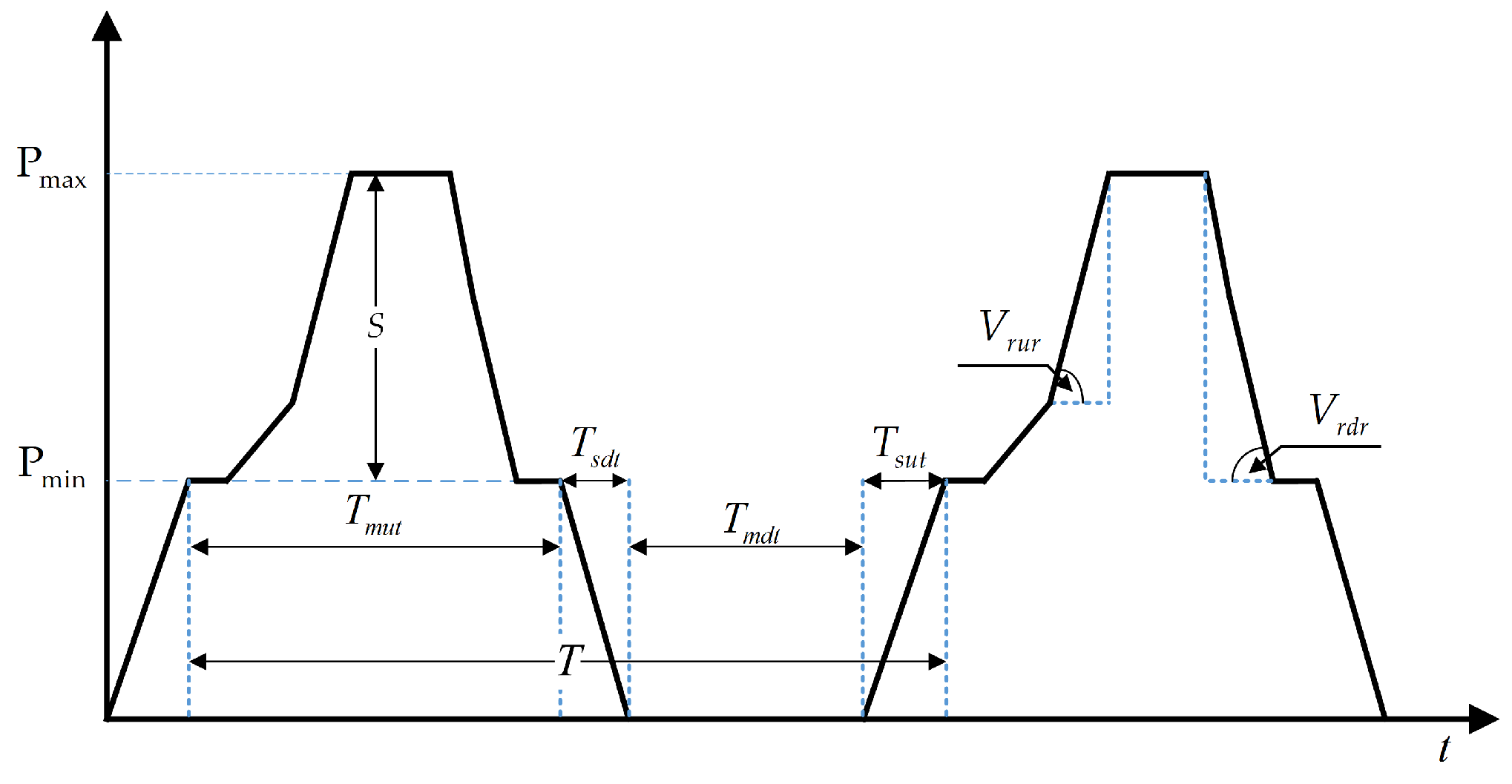
2.1. Technical Characteristics

The flexible technical characteristics of the TPU are mainly constrained in both time and output. In reference [8], eight indicators, namely, the operating range, ramping capabilities, start-up and shut-down times, and minimum up and down times of the generator were considered to characterize the technical characteristics of the unit’s flexibility. Although [8] analyzed the correlations between the indicators, the continuity of time was ignored. Because the operation of each unit is a continuous process, it is impossible for power units to start or stop in two consecutive time periods. Dispatchers are more concerned about how long the generator units can be flexibly adjusted to meet the imbalance of the power system. Therefore, this paper improves the indicators of the literature [8], by combining the indicators of start-up and shut-down time and minimum up and down time into one unified whole. The flexible technical characteristics of the TPU are shown in Figure 1:

where P_max is the maximum capacity, P_min is the minimum stable generation level, T_mut is the minimum up time, T_sdt is the shut-down time, T_mdt is the minimum down time, T_sut is the start-up time, V_rur is the maximum ramp up speed, and V_rdr is the maximum ramp down speed of the TPU.

2.1.1. Adjustable Capacity

The regulation capacity of TPU is defined as the steady adjustment of the unit output to meet the fluctuations in the net load under normal operating conditions, and the range of the adjustment output is the adjustable capacity. It is generally believed that the regulation capacity (S, as shown in Figure 1) of TPU is the rated capacity minus the minimum stable generation level:

$$S=P_{\max }-P_{\min }.$$

(1)

2.1.2. Ramping Rate

With the access to large-scale volatility power supplies, conventional generators require faster adjustment speeds in response to frequent changes in net load. The ramping rate is directional and has a close relationship with the time scale and operating conditions of the unit. The insufficient of each direction of ramping may cause an imbalance in the power system. Hence, in response to frequent fluctuations in net load, the ramping rate (V) can be characterized as the minimum absolute value of the ramp up and down speed:

$$V=\min \{\left|V_{rur}\right|,\left|V_{rdr}\right|\}.$$

(2)

2.1.3. Adjustment Period

As a result of high penetration fluctuating power in a power system, the unit sometimes needs to quickly start and stop to meet the requirements of the system. However, unlike energy storage, the start and stop of thermal power units is constrained by many factors. On the one hand, due to economic and security constraints, traditional generators must maintain a period of online operation after power-on to satisfy operating and maintenance costs. On the other hand, in order to prevent thermal stress and other factors from reducing the life of the unit, the conventional TPU is kept off for a period of time after the shutdown. The adjustment period (T) of a thermal unit is closely related to the start-up time, shut-down time, and the minimum up and down times of the unit. T (Figure 1) can be defined as the minimum time interval which begins at the moment the TPU starts up and goes until the P_min and ends at the next moment the TPU starts move to P_min:

$$T=\min (T_{sut}+T_{mut}+T_{sdt}+T_{mdt}).$$

(3)

2.2. Economic Characteristics

2.2.1. Operation Costs

In the power grid economic dispatching problem, the TPU peak regulation usually includes three stages [26]: regular peak regulation (RPR), deep peak regulation without oil (DPR), and deep peak regulation with oil (DPRO). DPRO includes RPR and DPR and involves a variety of factors. The peak energy cost (F) of the TPU is as follows:

$$F=f(P)+C_{\cos t}(P)+C_{oil}+C_{env}(P)$$

(4)

$$f(P)=(a{P}^2+bP+c)\times C_{coal }$$

(5)

where a, b, and c are the coefficients of the unit’s consumption characteristic function, and their values are related to the unit type, boiler type, and coal quality. C_coal is the unit coal price of the current season. C_cost is loss cost of the unit. C_oil is the cost of fuel consumption. C_env is the additional environmental cost.

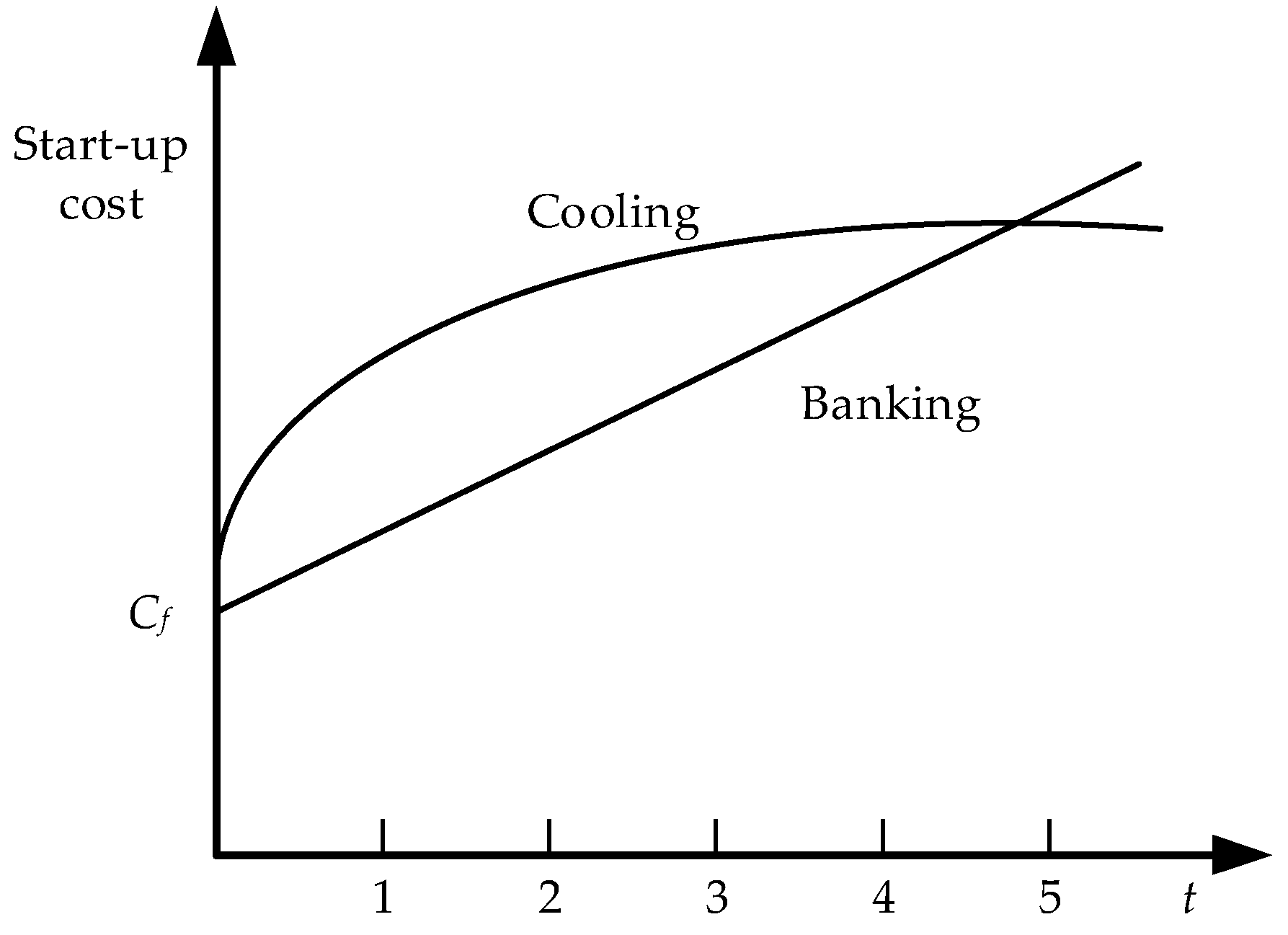
2.2.2. Start-up Costs

The start-up costs of a TPU are related to the pressure and temperature of the turbine at startup. Time-dependent start-up costs is shown in Figure 2 [27].

As shown in Figure 2, the cost (U) of a TPU is a function of time:

$$U=\{\begin{array}{cc}{C}_c(1-{\epsilon }^{-t/\alpha })\times F_c+C_f\hfill & cooling\hfill \\ C_t\times t\times F_c+C_f\hfill & banking\hfill \end{array}$$

(6)

where C_c is the cost of the cold start, F_c is the fuel cost, C_f is the fixed cost, and C_t is the cost of maintaining the unit temperature.

2.3. Selection of Flexibility Indexes of TPU

In this paper, the adjustable capacity (S) of the TPU, the ramping rate (V), the adjustment period (T), the operation costs (C) and the start-up costs (U) are selected to evaluate the flexibility of the unit. Any of these evaluation indicators reflect and characterize the flexibility of TPU. Figure 3 compares the five flexibility indicators of the three different units with three thermal power units (50 MW gas unit, and 100 MW and 300 MW coal-fired units) within the scope of an actual power grid.

It can be seen from Figure 3 that a gas turbine with a rated capacity of 50 MW is superior in the adjustment period and in terms of economic indicators, but its adjustable capacity and ramping rate are limited. The 300 MW unit with its larger rated capacity has a better adjustable capacity and ramp rate than the 100 MW unit, but the adjustment period is longer and the economy is poor. It is difficult to judge the overall flexibility of the unit through a single indicator. For this reason, a TPU flexibility evaluation index system is needed to evaluate the comprehensive flexibility of the TPU.

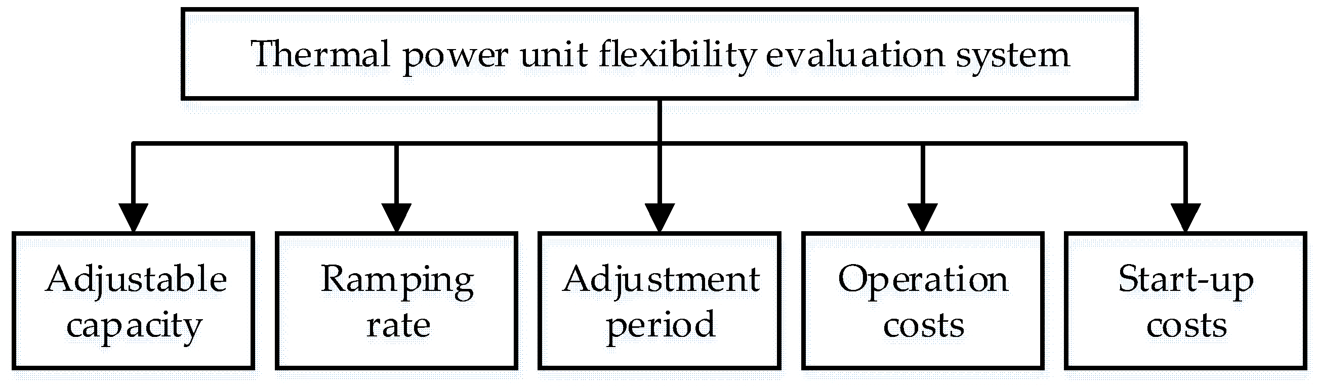
3. TPU Flexibility Evaluation Index System

The method of multiple indexes was used to analyze the TPU flexibility, because it is closely related with many factors. Composite metrics have been extensively used in diverse fields, such as economic, environmental, and technological performance, and have recently been applied to the power industry [28]. Reference [8] used AHP to quantitatively evaluate the flexibility resources of a power system, but did not consider the objective aspect. In this paper, the AHP-entropy method was used to calculate the index weight of TPU flexibility considering both subjective and objective factors. On the one hand, through the subjective judgment of experts by AHP, the knowledge and work experience can be better integrated into the weight coefficient decision. On the other hand, based on the amount of information provided by each indicator of the TPU, the entropy method was used to determine the objective index weight. Then, the comprehensive weight model was established.

3.1. Analytic Hierarchy Process

Saaty [29] provided a theoretical foundation for the AHP, that is, a decision support tool which can be used to solve complex decision problems by taking into account tangible and intangible aspects. The analytic hierarchy process (AHP) is generally divided into the following four steps:

• Establish a hierarchy, as shown in Figure 4.
• Construct a comparison judgment matrix (A).

  $$A={(a_{ij })}_{n\times n}=\left[\begin{array}{cccc}{a}_{11}& a_{12}& \cdots & a_{1n}\\ a_{21}& a_{22}& \cdots & a_{2n}\\ ⋮& \cdots & \cdots & ⋮\\ a_{n1}& a_{n1}& \cdots & a_{nn}\end{array}\right]$$

  (7)

  where a_ij is the pairwise comparison rating between indicator i and indicator j. The pairwise comparison scale is shown in

  Table 1. The analytic hierarchy process (AHP) pairwise comparison scale.

  Numerical Values	Verbal Scale	Explanation
  1	Equal importance of both elements	Two elements contribute equally
  3	Moderate importance of one indicator over another	Experience and judgment favor one indicator over another
  5	Strong importance of one indicator over another	An indicator is strongly favored
  7	Very strong importance of one indicator over another	An indicator is very strongly dominant
  9	Extreme importance of one indicator over another	An indicator is favored by at least an order of magnitude
  2, 4, 6, 8	Intermediate values	Used to compromise between two judgments

  [29].
• Consistency test of the judgment matrix.
  The quantitative indicator that measures the degree of inconsistency is called the consistency indicator (CI):

  $$CI=\frac{{\lambda }_{\max }-n}{n-1}$$

  (8)

  where λ_max is the largest eigenvalue of the comparison judgment matrix, and the expert’s judgment becomes inconsistent with an increase in the number of indicators. In order to measure the CI standard, Satty et al. proposed the use of the random consistency ratio (CR < 0.1) to correct the consistency index [29].
• Calculate the weight of the indicator.
  The formulas for calculating the weight of each index using the weight vector calculation method of the product square root method are as follows:

  $$r_i=\sqrt[n]{({\displaystyle \prod _{j=1 }^n{a}_{ij}})} i=1,2,\cdots ,n$$

  (9)

  $$p_j=r_j/{\displaystyle \sum _{k=1 }^n{r}_k, j=1,2,\cdots ,n}$$

  (10)

  where: r_i is the geometric mean of the elements of each row in the judgment matrix A; p_j is the weight coefficient of index j.

3.2. Entropy Method

Entropy was originally a term used in thermodynamics, and it is a measure of information in information theory. The entropy method mainly uses observation data provided by the index to avoid the disadvantages of the subjective weighting method. It is a method of objective weighting. The method of determining the weight coefficient is given by using the concept of entropy as follows:

A m × n observation data matrix (u_ij) was established, and represents the observation data of the j-th index of the evaluation object (i). For indicator j, the greater the difference in u_ij, the more information that indicator j contains, which means the weighting factor of indicator j is greater. The steps for determining the index weight coefficient by the entropy method are as follows:

• Calculate the feature weight of the i-th evaluated object under the j-th index:

  $$h_{ij}=u_{ij}/{\displaystyle \sum _{i=1}^m{u}_{ij}}.$$

  (11)
• Calculate the entropy value (e_j) of the j-th indicator:

  $$e_j=-k{\displaystyle \sum _{i=1}^m{h}_{ij}\ln \left(h_{ij}\right)}.$$

  (12)
• Calculate the difference coefficient matrix of the indicator:

  $${\beta }_j=1-e_j.$$

  (13)
• Calculate the weight coefficient:

  $$q_j={\beta }_j/{\displaystyle \sum _{k=1}^n{\beta }_k,j=1,2,\cdots ,n}.$$

  (14)

3.3. Construction of the Comprehensive Weighting Model

The AHP mainly reflects the subjective judgment of the evaluator on the flexibility of the TPU, and the entropy method dynamically analyzes the observation data of all units in the dispatching range to make the result more objective. Both methods have their own advantages. The weight coefficients calculated by these two methods are more objective and scientific. The steps for the construction of the comprehensive weighting model are as follows:

• This paper uses the commonly used Lagrangian multiplier method for comprehensive empowerment:

  $$z_j=\sqrt{p_j{q}_j }/{\displaystyle \sum _k^n\sqrt{p_k{q}_k}}$$

  (15)

  where w_j is the calculated comprehensive weight coefficient.
• The assembly model used in this paper is a linear “addition” integrated assembly model.

  $$Fle{x}_i={\displaystyle \sum _{j=1 }^n{z}_j}{x}_{ij}$$

  (16)

  where Flex_i is the comprehensive flexibility evaluation score of TPU i; n is the total number of indicators; x_ij is the observation value of index j of TPU i.

4. Optimization Scheduling Model Considering TPU Flexibility

4.1. Objective Function and Constraints

The conventional optimization scheduling model allocates the output power of TPU reasonably under the premise of satisfying the load and system operation constraints, so that the total power generation cost in the scheduling period is minimized. However, due to the large-scale WP grid connection, the conventional economic dispatch model has difficulty meeting the dual uncertainty of WP and load. In order to ensure the safe and stable economic operation of the power system, this paper proposes a power system optimization scheduling model that takes the flexibility of each TPU into account.

4.1.1. Objective Function

$$\min f_{th }={\displaystyle \sum _{t=1}^T{\displaystyle \sum _{i=1}^N{F}_{i,t}{I}_{i,t}+U_i}}{I}_{i,t}\times (1-I_{i,t-1})$$

(17)

$$\max f_f={\displaystyle \sum _{t=1 }^T{\displaystyle \sum _{i=1}^{N}Fle{x}_i{I}_{i,t}}}$$

(18)

where f_th is the conventional economic dispatch target and f_f is the flexibility dispatch target; F_i,t is the operating cost of unit i during t period, I_i,t is the binary integer variable which reflects the opening and stopping state of the unit i in the period t, and U_i is the starting cost of unit i. Flex_i in Equation (18) represents the flexibility score of the ith TPU. Through the scheduling models of Equations (17) and (18), it is possible to achieve a higher total TPU flexibility supply for a small power generation cost. Equations (17) and (18) represent a dual target optimization problem, in which the direction of optimization of the two objective functions is opposite. In order to solve the dual target optimization problem, the linear model (Equations (19)) commonly used in engineering was utilized in this paper:

$$\begin{array}{c}\min T=\alpha f_f^{*}+\beta f_{th }^{*}\\ \alpha +\beta =1\end{array}$$

(19)

where T is the total target; $f_{th}^{\ast }$ and $f_f^{\ast }$ are the normalized and consistent single target values; and α and β are the weights of targets f_f and f_th;

The advantage of using a linear model is that the model is simple and easy to solve. The mainly contribution of Equation (19) is that the model provides two open source parameters to the dispatching department which can adjust the parameters according to the actual conditions.

4.1.2. Restrictions

(1) Load balancing constraint.

$${\displaystyle \sum _{i=1 }^N(P_{G_{i,t}})I_{i,t}=}{P}_{Lt}-P_{Wt}$$

(20)

where P_Gi,t is the active power of unit i in period t; P_Lt is the predicted value of load in period t; and P_Wt is the total predicted value of wind power in the scheduling range of period t.

(2) Unit power generation limit constraint.

$$P_{Gi }^{\min }{I}_{i,t}\le P_{Gi,t}\le P_{Gi}^{\max }{I}_{i,t}$$

(21)

where $P_{Gi}^{\max }$ and $P_{Gi}^{\min }$ are the rated capacity and minimum stable output of unit i, respectively.

(3) System backup constraint.

$${\displaystyle \sum _{i=1 }^N{P}_{{}_{Gi}}^{\max }{I}_{i,t}\ge }{P}_{Lt}-P_{Wt}+P_{Rt}$$

(22)

where: P_Rt is the spare capacity of t period t.

(4) Minimum on–off time constraint.

$$(X_{{ }_{i,t-1}}^{on}-T_i^{on})(I_{{}_{i,t-1}}-I_{{}_{i,t}})\ge 0$$

(23)

$$(X_{{ }_{i,t-1}}^{off}-T_i^{off})(I_{{}_{i,t}}-I_{{}_{i,t-1}})\ge 0$$

(24)

where $X_{i,t-1}^{on}$ and $X_{i,t-1}^{off}$ are the times of continuous start (stop) of unit i to the dispatch period (t − 1); $T_i^{on}$ and $T_i^{off}$ are the minimum on (off) times of unit i.

(5) Ramping constraint of the unit.

$$P_{G_{i,t }}-P_{G_{i,t-1}}\le U{R}_i$$

(25)

$$P_{G_{i,t-1 }}-P_{G_{i,t}}\le D{R}_i$$

(26)

where: UR_i and DR_i are the limits of the amounts of active power increase and decrease of unit i, respectively.

4.2. System Flexibility Assessment

The renewable energy represented by WP is essentially the dispersion of the spatial scale and the random fluctuation uncertainty of the time scale. Moreover, the random uncertainty of wind energy varies with different seasonal, climatic, local meteorological, and geographical conditions. The dispatching department must grasp the fluctuation law of WP within its dispatching range, and should make power generation schedule have strong flexibility under the background that the WP prediction accuracy is not high at this stage.

4.2.1. System Flexibility Assessment Indicators

The flexibility demands of the system are divided into the upward adjustment flexibility demand {upd_t} and the downward adjustment flexibility demand {dnd_t}, which is mainly related to the changes in the system’s net load (P_net):

$$\begin{array}{l}\{\begin{array}{l}up{d}_t=P_{net,t+1.}-P_{net,t}\\ dn{d}_t=0\end{array} P_{net,t+1}-P_{net,t}>0\\ \{\begin{array}{l}up{d}_t=0\\ dn{d}_t=P_{net,t}-P_{net,t+1}\end{array} P_{net,t+1}-P_{net,t}\le 0\end{array}.$$

(27)

After the power generation plan has been completed, the dispatching department needs to evaluate the adaptability of the power generation plan.

In this paper, we use the two indicators proposed in reference [30] (upward flexibility deficiency probability P_UFNS and downward flexibility deficiency probability P_DFNS) to evaluate the system’s flexibility:

$$\{\begin{array}{l}{P}_{UFNS,t }=\mathrm{Pr}\{R{U}_t<up{d}_t\}\\ R{U}_t=\min [{\displaystyle \sum _{i=1}^{N_g}(P_{Gi}^{\max }-}{P}_{Gi,t}^{}),{\displaystyle \sum _{i=1}^{N_g}(U{R}_i\times \Delta T)}]\end{array}$$

(28)

$$\{\begin{array}{l}{P}_{DFNS,t }=\mathrm{Pr}\{R{D}_t<dn{d}_t\}\\ R{D}_t=\min [{\displaystyle \sum _{i=1}^{N_g}(P_{Gi,t}^{}-P_{Gi}^{\min }}),{\displaystyle \sum _{i=1}^{N_g}(D{R}_i\times \Delta T)}]\end{array}$$

(29)

where RU_t and RD_t are, respectively, the upward adjustment flexibility supply and the downward adjustment flexibility supply provided by TPU, during the system’s scheduling interval of Δt at time t.

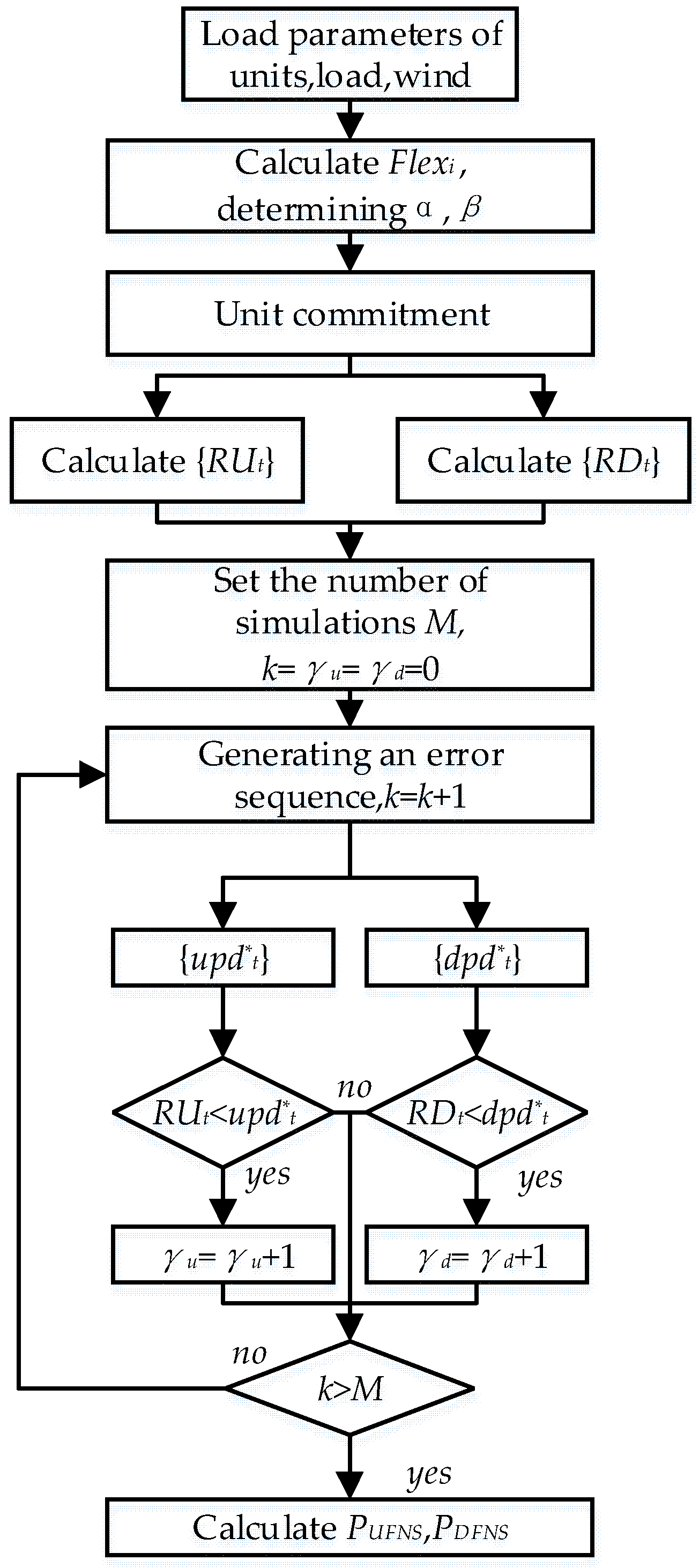
4.2.2. Power Generation Plan Flexibility Assessment Process

This section presents a practical algorithm that is based on the Monte Carlo algorithm to assess the flexibility of a power generation plan. The process is shown in Figure 5.

The steps are as follows:

(1)

Input the unit parameters, the comprehensive flexibility evaluation value, and the load and wind data and determine the flexibility factor (α) in Equation (19).

(2)

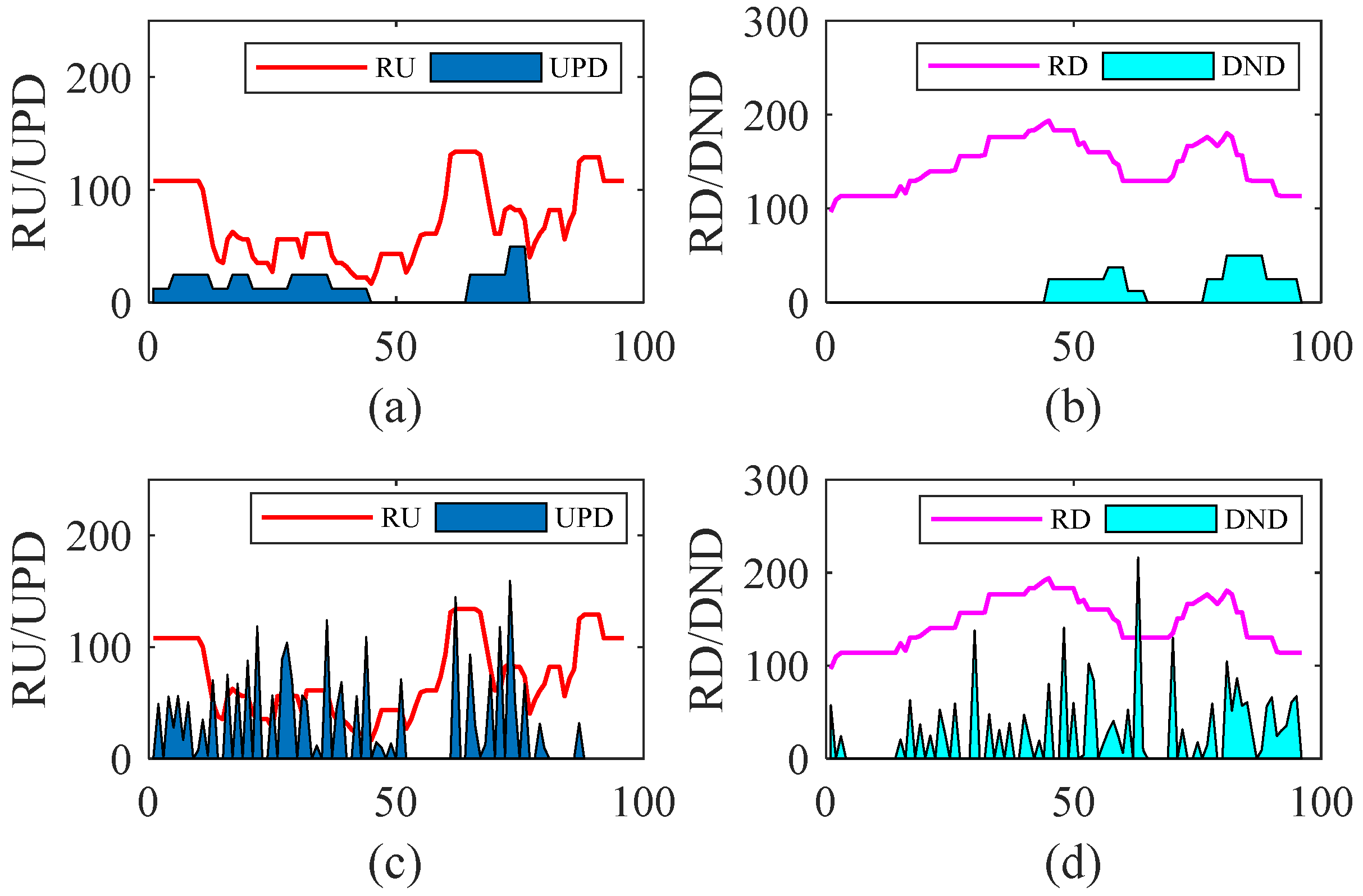
Based on the wind power and load forecast data, determine the power generation plan, obtain the upward adjustment flexibility supply ({RU_t}) and the downward adjustment flexibility supply ({RD_t}), and set the simulation frequency (M).

(3)

Based on Equation (27), obtain the up-regulated flexibility requirement sequence ({upd_t}) and down-regulated flexibility requirement sequence ({dnd_t}) during the scheduling period.

(4)

Using the WP historical prediction error distribution within the scheduling range, use the Monte Carlo simulation to generate the prediction error timing ({ε_t}).

(5)

According to the WP prediction error sequence ({ε_t}) generated in step 4, modify the up-regulated flexibility requirement sequence and down-regulated flexibility requirement sequence to obtain ({$up{d}_t^{\ast }$}) and ({$dn{d}_t^{\ast }$}).

(6)

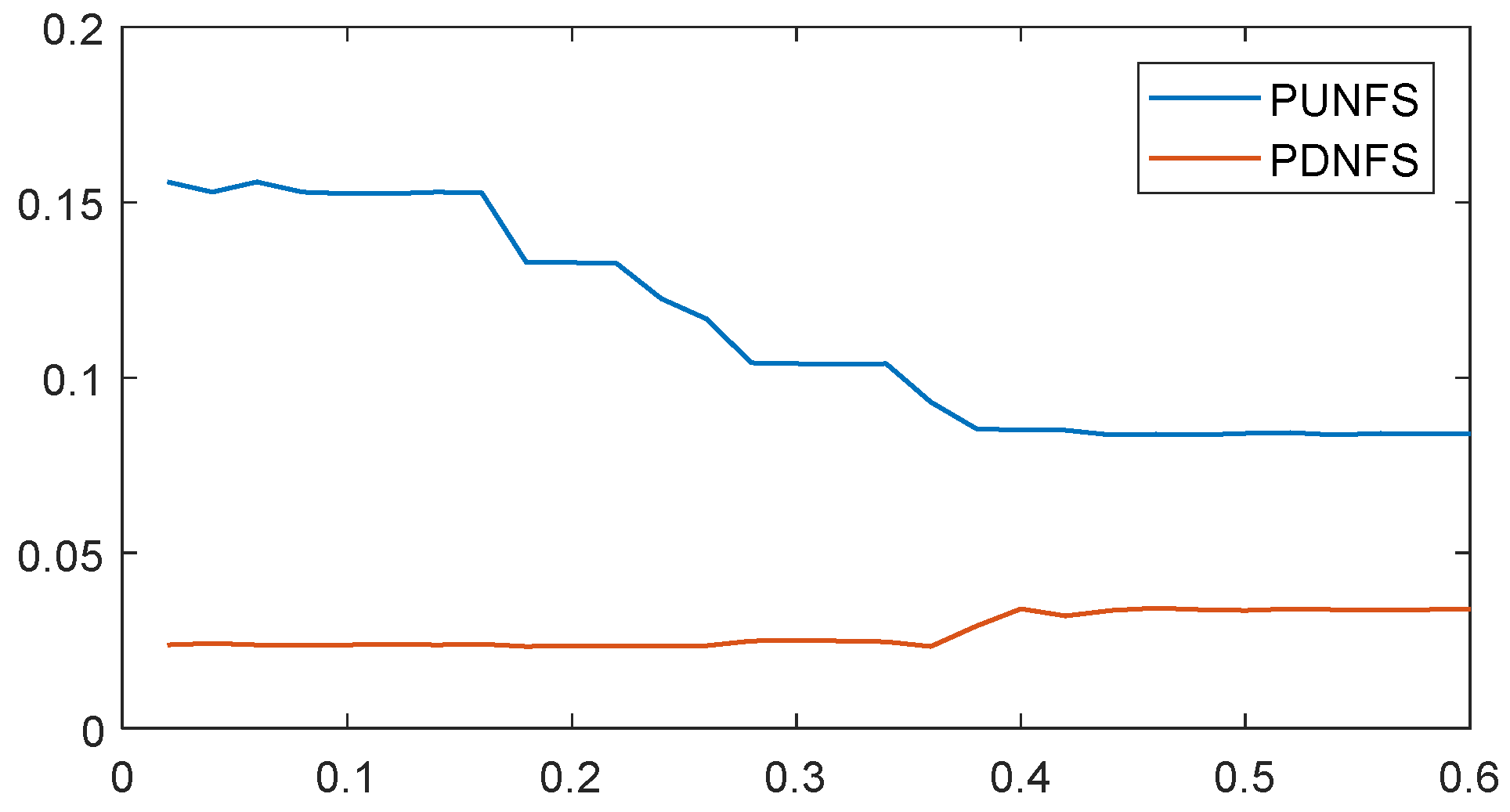
Set the intermediate variables γ_u and γ_d to record the simulation results, and finally get the upward flexibility deficiency probability (P_UFNS) and downward flexibility deficiency probability (P_DFNS).

5. Case Study

The data used for the case was based on a 10-unit system [31] and the data parameters are provided in Appendix A. Since the data parameters of the 10 units provided by reference [31] do not provide the data for unit ramping, this paper used the 15% rated capacity of the unit to simulate the maximum up and down adjustment capacities in a 15-min period. And this article expands the 24-point load data [31] to 96 points by interpolation to cope with 15-min period WP fluctuations. The solution of the unit commitment was implemented by the Cplex12.8 solvers.

5.1. Unit Flexibility Evaluation

Eight experts were invited to participate in this evaluation. According to the relevant national standards, the experts provided scores on the basis of the comparison of two indexes that represented the importance of the various factors. Then, judgment matrix A was established:

$$\mathrm{A}=\left[\begin{array}{ccccc}1& 1& 1/3 & 3& 2\\ 1& 1& 1/3& 2& 2\\ 1/3& 3& 1& 4& 3\\ 1/3& 1/2& 1/4& 1& 1/3\\ 1/2& 1/2& 1/3& 3& 1\end{array}\right]$$

The testing of CR < 0.1 showed that it meets the requirements for consistency. After loading the 10 TPU parameters, the comprehensive weights of the five indicators were obtained using Equations (9)–(16).

Table 2. Comprehensive weights of the indicators.

Index	S	V	T	C	U
Subjective weight	0.228	0.210	0.327	0.084	0.150
Objective weight	0.195	0.199	0.198	0.180	0.227
Comprehensive weight	0.222	0.209	0.322	0.076	0.171

lists the comprehensive weights of the indicators.

It can be seen from Table 2 that T is the most important indicator affecting the flexibility of the TPU. Because the economical operation of the unit was considered in the process of economic dispatching, the weight of the unit’s operational economic indicators weakened during the flexibility assessment of the unit. The final flexibility quantitative scores of the 10 units are shown in

Table 3. Comprehensive weight of the indicators.

Index	1	2	3	4	5	6	7	8	9	10
Pmax	455	455	130	130	162	80	85	55	55	55
Flex	126.50	126.61	60	60.14	69.15	66.15	60.89	143.58	143.51	143.46

:

As can be seen from Table 3, the three 55 MW units can quickly start and stop with the highest flexibility. However, due to different starting costs and operating costs, the flexibility of the three units is also different.

5.2. The Impacts of Uncertainty on the System

After large-scale WP is connected to the grid, the system’s net load fluctuates more severely. In this paper, the prediction error of 105,216 time points of a power grid in Northeast China from 2015 to 2017 was used as the error empirical distribution to simulate the uncertainty of wind power, as shown in Figure 6.

The greater the proportion of wind power access, the flexibility the demand needed is. The unit commitment strategy changes when α value in the unit commitment target is changed, so the unit commitment strategy is more adaptable. The configuration parameters of the wind power access ratio (k) and flexibility target weight (α) are shown in

Table 4. Configuration parameters.

Strategies	S1	S2	S3	S4
k	0	10%	10%	10%
α	0	0	0.2	0.35

.

In order to cope with the impact of wind power uncertainty, this paper adopts four configuration strategies. The purpose was to explore the impact of TPU flexibility on the uncertainty of the adaptation plan of the dispatching department. Figure 7a,b are the bidirectional flexibility supply and demand maps of the system without WP.

The space for net load upward adjustment is very tiny, and it is prone to a lack of upward flexibility supply after adding WP (Figure 7c). The downward adjustment space of the net load is very large, and the downward flexibility supply is sufficient (Figure 7d). A comparison of the results of Figure 7a,c shows that the 10-unit system is prone to imbalance due to the lack of upward flexibility supply. Considering only the economic dispatch, the schedule lacks flexibility and is prone to outage and wind curtailment. The reason why Figure 7 appears is that the scheduling plan cannot cope with the prediction error of wind power. The flexibility supply of TPU is limited by the economic scheduling plan.

5.3. The Impacts of the TPU Flexibility on the System

In order to ensure the safe and stable economic operation of the power system, strategies S3 and S4 were used which released the TPU’s flexible adjustment space. Comparison of strategies of S2, S3 is shown in Figure 8.

As shown in Figure 8a, the upward adjustment flexibility supply of Strategy 3 is better than Strategy 2. By using the model proposed by this paper, the TPU’s upward flexible adjustment space is increased. Comparison of the downward adjustment flexibility supply is shown in Figure 8b. Strategy 3 is better than Strategy 2 when the net load is large, but when the net load is low, the situation is reversed. The reason why the RD decreases in Strategy 3 is that the units’ minimum operating constraints limit the RD while providing RU. However, the two indicators, P_UNFS and P_DNFS, are better than Strategy 2 compared to Strategy 3.

Using Figure 5, P_UNFS and P_DNFS were obtained, and the comparison of strategies S2, S3, and S4 are shown in Figure 9. P_UNFS and P_DNFS indicators experienced different degrees of decline. The Equation (19) provide two open source parameters to the dispatching department which can adjust the parameters according to actual conditions. When the flexibility of TPU was considered, the system’s indicators of P_UNFS and P_DNFS decreased, as shown in Figure 9.

5.4. Sensitivity Analysis

Due to the power structure and load level of the system, the flexibility of the system is limited. As shown in Figure 10, as the value of the adjustment (α) continuously increases, the two indicators P_UNFS and P_DNFS do not infinitely decrease. Convergence occurs near α = 0.4, which reaches the limit of the flexibility of the system.

As the installed capacity of wind power continues to expand, it is necessary to change the power structure within the scheduled areas, and increase the proportion of flexible adjustment of the unit. Increasing the proportion of flexible adjustment units is an effective method to reduce P_UNFS and P_DNFS, which have greater uncertainty adaptability.

6. Conclusions

In order to alleviate the uncertainty caused by large-scale WP grid-connected systems, this paper proposed an optimal scheduling method that considers the flexibility of the TPU. (1) Based on the AHP-entropy method, a comprehensive evaluation system for unit flexibility was established based on five variables: adjustable capacity, ramping rate, adjustment period, operation costs and start-up costs of TPU; (2) The flexibility of the unit was considered in the traditional economic dispatch optimization model, and the multi-objective optimization scheduling model was established with the aims of system economy and flexibility. Through linearization processing, the transformation from multi-target to single target was realized; (3) The example analysis showed that the proposed optimal scheduling method can effectively alleviate the imbalance between supply and demand in bidirectional flexibility of the system.

The shortcomings and limitations of the model is that the evaluation of TPU flexibility does not take the impacts of environmental factors into account. There are many flexibility resources, but this article only considered thermal power units. The next step in this paper is to evaluate the flexibility of hydropower and nuclear power plants to take each unit’s flexibility into account during the scheduling process.

References

1. Global Statistics. Available online: http://gwec.net/global-figures/graphs (accessed on 8 July 2018).
2. 2017 Wind Power Grid Operation. Available online: http://www.nea.gov.cn/2018-02/01/c_136942234.htm (accessed on 19 August 2018).
3. International Energy Agency. Empowering Variable Renewables-Options for Flexible Electricity Systems; OECD Publishing: Paris, France, 2009; pp. 13–14. [Google Scholar]
4. Xiao, D.; Wang, C.; Zeng, P. A survey on power system flexibility and its evaluations. Power Syst. Technol. 2014, 38, 1569–1576. [Google Scholar]
5. Lannoye, E.; Flynn, D.; O’Malley, M. Evaluation of power system flexibility. IEEE Trans. Power Syst. 2012, 27, 922–931. [Google Scholar] [CrossRef]
6. Lannoye, E.; Flynn, D.; O’Malley, M. Power system flexibility assessment; state of the art. In Proceedings of the IEEE Power and Energy Society General Meeting, San Diego, CA, USA, 22–26 July 2012. [Google Scholar]
7. Lannoye, E.; Flynn, D.; O’Malley, M. Transmission, variable generation and power system flexibility. IEEE Trans. Power Syst. 2015, 30, 57–66. [Google Scholar] [CrossRef]
8. Oree, V.; Hassen, S.Z.S. A composite metric for assessing flexibility available in conventional generators of power systems. Appl. Energy 2016, 177, 683–691. [Google Scholar] [CrossRef]
9. Exposito, A.G.; Santos, J.R.; Romero, P.C. Planning and Operational Issues Arising from the Widespread Use of HTLS Conductors. IEEE Trans. Power Syst. 2007, 22, 1446–1455. [Google Scholar] [CrossRef]
10. Wydra, M. Performance and Accuracy Investigation of the Two-Step Algorithm for Power System State and Line Temperature Estimation. Energies 2018, 11, 1005. [Google Scholar] [CrossRef]
11. Kubik, M.L.; Coker, P.J.; Barlow, J.F. Increasing thermal plant flexibility in a high renewables power system. Appl. Energy 2015, 154, 102–111. [Google Scholar] [CrossRef]
12. Eser, P.; Singh, A.; Chokani, N.; Abhari, R.S. Effect of increased renewables generation on operation of thermal power plants. Appl. Energy 2016, 164, 723–732. [Google Scholar] [CrossRef]
13. Van den Bergh, K.; Delarue, E. Cycling of conventional power plants: technical limits and actual costs. Energy Convers. Manag. 2015, 97, 70–77. [Google Scholar] [CrossRef]
14. Yasuda, Y.; Ardal, A.R.; Carlini, E.M.; Estanqueiro, A.I.; Flynn, D.; Gomez-Lazaro, E.; Holttinen, H.; Kiviluoma, J.; Van Hulle, F.; Kondoh, J.; et al. Flexibility chart: evaluation on diversity of flexibility in various areas. In Proceedings of the 12th International Workshop on Large-Scale Integration of Wind Power into Power Systems As Well As on Transmission Networks for Offshore Wind Power Plants, London, UK, 22–24 October 2013. [Google Scholar]
15. Kirby, B.; Milligan, M.R. A Method and Case Study for Estimating the Ramping Capability of a Control Area or Balancing Authority and Implications for Moderate or High Wind Penetration; 2005. Available online: http://www.nrel.gov/docs/fy05osti/38153.pdf (accessed on 19 August 2018).
16. Mustafa, M.A.; Al-Bahar, J.F. Project risk assessment using the analytic hierarchy process. IEEE Trans. Eng. Manag. 1991, 38, 46–52. [Google Scholar] [CrossRef]
17. Padhy, N.P. Unit commitment—A bibliographical survey. IEEE Trans. Power Syst. 2004, 19, 1196–1205. [Google Scholar] [CrossRef]
18. Saravanan, B.; Das, S.; Sikri, S.; Kothari, D.P. A solution to the unit commitment problem—A review. Front. Energy 2013, 7, 223–236. [Google Scholar] [CrossRef]
19. Wind Power Integration in Liberalized Electricity Markets (Wilmar) Project. Available online: www.wilmar.risoe.dk (accessed on 19 August 2018).
20. Tuohy, A.; Meibom, P.; Denny, E.; O’Malley, M. Unit commitment for systems with significant wind penetration. IEEE Trans. Power Syst. 2009, 24, 592–601. [Google Scholar] [CrossRef] [Green Version]
21. Wu, L.; Shahidehpour, M.; Li, Z. Comparison of scenario-based and interval optimization approaches to stochastic SCUC. IEEE Trans. Power Syst. 2012, 27, 913–921. [Google Scholar] [CrossRef]
22. Bai, W.; Lee, D.; Lee, K.Y. Stochastic dynamic AC optimal power flow based on a multivariate short-term wind power scenario forecasting model. Energies 2017, 10, 2138. [Google Scholar] [CrossRef]
23. Growe-Kuska, N.; Heitsch, H.; Romisch, W. Scenario reduction and scenario tree construction for power management problems. In Proceedings of the IEEE Bologna Power Tech Conference, Bologna, Italy, 23–26 June 2003. [Google Scholar] [Green Version]
24. Hu, M.; Hu, Z. Optimization scheduling method for power systems considering optimal wind power intervals. Energies 2018, 11, 1710. [Google Scholar] [CrossRef]
25. Li, Z.; Jin, T.; Zhao, S.; Liu, J. Power system day-ahead unit commitment based on chance-constrained dependent chance goal programming. Energies 2018, 11, 1718. [Google Scholar] [CrossRef]
26. Lin, L.; Zou, L.; Zhou, P.; Tian, X. Multi-angle Economic Analysis on Deep Peak Regulation of Thermal Power Units with Large-scale Wind Power Integration. Autom. Electr. Power Syst. 2017, 41, 21–26. [Google Scholar]
27. Wood, A.J.; Wollenberg, B.F. Power Generation, Operation, and Control, 2nd ed.; Wiley: New York, NY, USA, 1996. [Google Scholar]
28. Shi, R.; Fan, X.; He, Y. Comprehensive evaluation index system for wind power utilization levels in wind farms in China. Renew. Sustain. Energy Rev. 2017, 69, 461–471. [Google Scholar] [CrossRef]
29. Saaty, T.L. Fundamentals of the analytic hierarchy process. In Analytic Hierarchy Process in Natural Resource and Environmental Decision Making: Fundamentals of the Analytic Hierarchy Process; Schmoldt, D.L., Kangas, J., Mendoza, G.A., Pesonen, M., Eds.; Kluwer Academic Publishers: Dordrecht, The Netherlands, 2001. [Google Scholar]
30. Li, H.; Lu, Z.; Qiao, Y.; Zeng, P. Large-scale wind power grid-connected power system operational flexibility assessment. Power Syst. Technol. 2015, 39, 1672–1678. [Google Scholar]
31. Kazarlis, S.A.; Bakirtzis, A.G.; Petridis, V. A genetic algorithm solution to the unit commitment problem. IEEE Trans. Power Syst. 1996, 11, 83–92. [Google Scholar] [CrossRef]
Figure 1. Flexibility of thermal power unit (TPU) technical characteristics.
Energies 11 02195 g001
Figure 2. Time-dependent start-up costs.
Energies 11 02195 g002
Figure 3. Comparison of five flexibility indicators of different units: (a) 50 MW gas unit and 100 MW coal-fired unit; (b) 100 MW and 300 MW coal-fired units.
Energies 11 02195 g003
Figure 4. Thermal power unit flexibility evaluation system.
Energies 11 02195 g004
Figure 5. Algorithm flowchart.
Energies 11 02195 g005
Figure 6. Wind power prediction error distribution.
Energies 11 02195 g006
Figure 7. The results of the comparison of the S1 and S2 strategies. (a) The comparison of the upward adjustment flexibility supply (RU) and the up-regulated flexibility requirement (UPD) of S1; (b) comparison of the downward adjustment flexibility supply (RD) and the down-regulated flexibility requirement DND of S1; (c) comparison of RU and UPD of S2; (d) comparison of RD and DND of S2.
Energies 11 02195 g007
Figure 8. Comparison of strategies of S2, S3. (a) Comparison of the RU; (b) Comparison of the RD.
Energies 11 02195 g008
Figure 9. Comparison of strategies of S2, S3 and S4. (a) Comparison of PUNFS; (b) Comparison of PDNFS.
Energies 11 02195 g009
Figure 10. Sensitivity analysis.
Energies 11 02195 g010