1. Introduction
Protection is one of the most critical and challenging problems when it comes to microgrid systems. Microgrids contain converter-interfaced distributed energy resources (DER) and loads along with traditional electric machinery. In the case of various faults within these architectures, the converters interfacing the DER provide limited fault current in comparison to the response of electric machinery [
1,
2,
3]. The maximum output current is typically clamped to 1–3 times the rated output current of the converter [
4]. This becomes even more problematic if the microgrid were to operate in islanded mode [
1,
2,
3]. Other reported microgrid concerns that can cause protection difficulty include the bi-directionality of power flow [
5], and the diversification of DERs [
6,
7].
When it comes to protecting the microgrid, traditional over-current protection is not a reliable method [
5]. A microgrid can experience a fairly wide range of fault current magnitudes and, thus, conventional overcurrent schemes are not effective for microgrid protection [
8]. In fact, lower available source currents will result in longer trip times or blinding [
6,
7]. Fault detection methods utilizing voltage sag information have been successfully demonstrated in the literature [
9]. However, microgrid fault detection cannot be based on voltage levels alone [
10], because renewables must meet low-voltage and high-voltage ride-through requirements specified in IEEE1547.
Most protection methods proposed in the literature depend on differential protection and a communication system in order to achieve suitable protection metrics which can be slow and very costly [
6,
7,
11]. Relying on communication degrades the reliability because the system becomes more prone to a single point of failure. The communication based approaches solve the protection problem by adjusting relay settings through online communication platforms. Examples are found in [
12,
13,
14] where an extensive communication infrastructure was developed to update the relay settings adaptively or a central supervisory protection unit is utilized. A combination of different protection approaches have been proposed in [
15] with differential protection being used as the main strategy. This method is costly and slow since it relies on other mechanisms as backup.
Other approaches make use of advanced signal processing algorithms. Research teams have utilized sequence components [
2], which fail in detecting balanced three-phase faults and are unreliable in the case of unbalanced conditions [
7,
16]. Some have used data mining approaches along with the differentials, which are complex methods, and also depend on communication [
17]. The same is true for traveling wave-based approaches [
18,
19]. Wavelet analysis has been proposed in [
20] and [
21]. In [
22], the authors developed a method based on analyzing non-stationary differential signals using the Hilbert Huang transform. This method is complex and suffers from unsatisfactory reliability and high cost due to the differential protection used. The authors in [
23] used differential protection as a foundation and tried to improve it by using Hilbert space and fuzzy processes. This method still suffers from the same cost and reliability issues as pure differentials due to the use of differentials. In [
24], the authors proposed a solution based on transient polarity comparison, which is based on a wavelet transform but requires a central communication network. Finally, the research team utilizes harmonic impedances to identify faults in [
25]. This approach is able to distinguish between high impedance faults and bolted faults.
Other techniques make use of external devices to elevate fault current magnitudes. In [
26], the authors have added a flywheel in the microgrid in order to boost fault currents and use traditional over-current protection. Such approaches can be costly and depend on the proper operation of the flywheel. The latest hardware solutions in the literature make use of phasor measurement units [
27,
28] and a digital central protection unit in [
27]. This approach protects radial and looped microgrids against various fault types with the capability of single-phase tripping but still requires communications.
A unique solution that does not fit within the general category of fault identifying techniques listed thus far is found in [
29], which makes use of the phase change that is established between measured current and voltage during faults (with loads located on the main bus). With distributed loads (located between the generation and the protection relay) in the system, this method can fail.
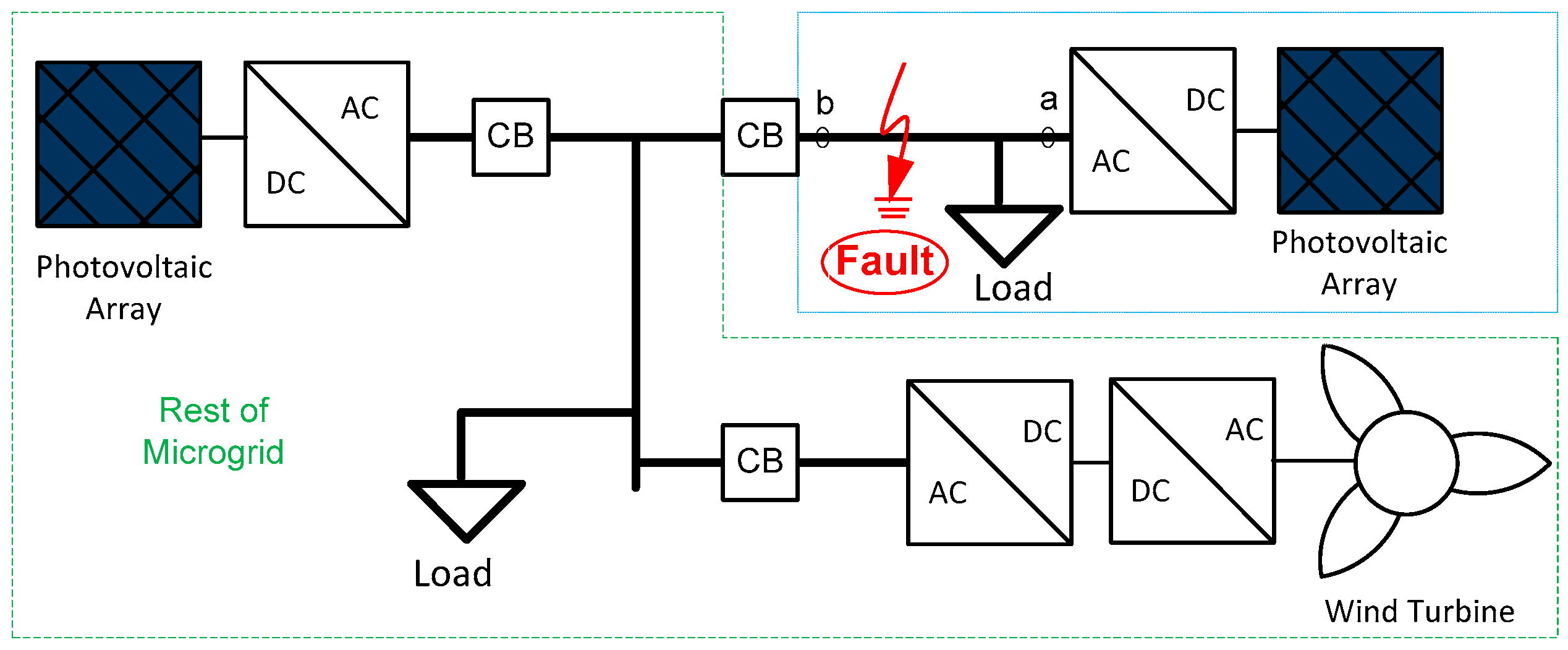
In this article a novel, model-based, communication-free fault detection method for inverter-based microgrids is proposed. The method can detect faults in the power transmission paths (feeders) of a microgrid (
Figure 1) regardless of the fault current level and the mode of operation (islanded or grid-connected). The developed scheme will overcome the issue of low fault levels that may cause breaker misoperation (nuisance tripping) or prevent the microgrid protection from tripping at all (blinding). It will not use central communication to allow the protection system to operate faster, be more reliable, and be less costly. Another main contribution of this article is the development of a mathematical framework to analyze and avoid blinding and nuisance tripping scenarios.
The rest of this paper is organized as follows: In the materials and methods section, the microgrid feeder model with different faulted and non-faulted conditions is given along with an explanation of the model-based fault detection approach. In the theory/calculation section, the mathematical proof of the ability to detect faults using one-sided measurement only (communication-less) will be provided and system constraints to avoid nuisance tripping and blinding will be given. In the simulations section, simulation results for the method using two-sided measurement (with communication) and the method using only one-sided measurement (no communication) will be provided. The simulation will demonstrate numerically that the proposed approach is able to distinguish between different conditions (faulted and non-faulted) in an inverter-dominated microgrid that produces low fault current levels. Finally, the article concludes and provides insight into the usefulness of the article with future work described.
2. Materials and Methods: Feeder Modelling and Fault Detection Approach
The major challenge of microgrid protection is that voltage and current levels alone cannot be used to detect faults. Hence, a method based on the structure (internal dynamics) of the microgrid is developed here. This approach is used because the circuit structure will change when a fault occurs within the microgrid. If we can identify the change in the internal system dynamics, we can detect faults. One approach to detect system changes is to have a prior knowledge of the possible system structures modeled as transfer functions, state-space descriptions or static models [
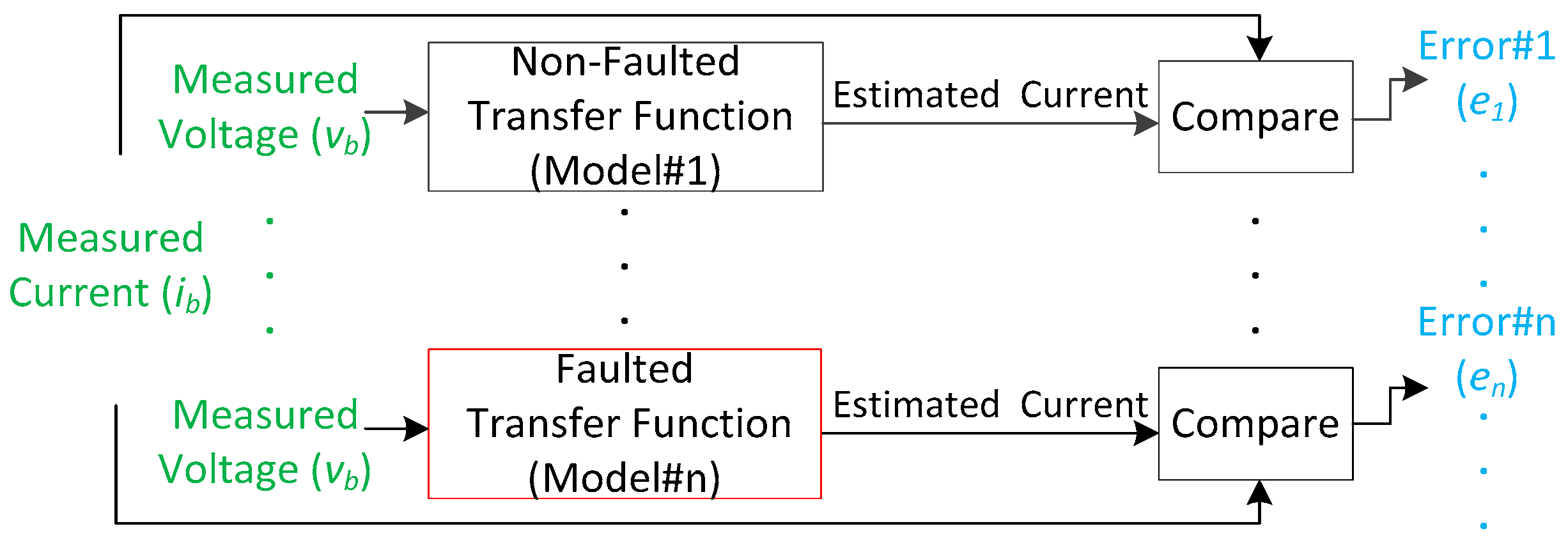
30]. Therefore, the different possible mathematical descriptions for different possible faulted conditions and a non-faulted condition must be derived. In the modeling process, the voltage of the system is treated as a system input and the current as a system output. Our methodology for identifying microgrid faults is depicted in
Figure 2. The communication-based approach utilizes two measurement locations at both ends of the transmission path (these occur at point
a and point
b in
Figure 1) as inputs to the protection apparatus. The communication-free approach exploits only one measurement located at the microgrid side (point
b only in
Figure 1) as an input to the protection apparatus. For both approaches, each model produces an estimated current which is compared to the measured current in real-time. When there is a match between a measured current and an estimated current, there will be a clear distinction between a faulted condition and a non-faulted condition. This will lead to the successful detection of a fault despite the low-current levels that the inverter-based sources produce during faults.
For the communication-free approach, the error between measured and estimated current could be large. This might hinder the operation of the protection system which can be avoided under certain system constraints derived in forthcoming sections of the article.
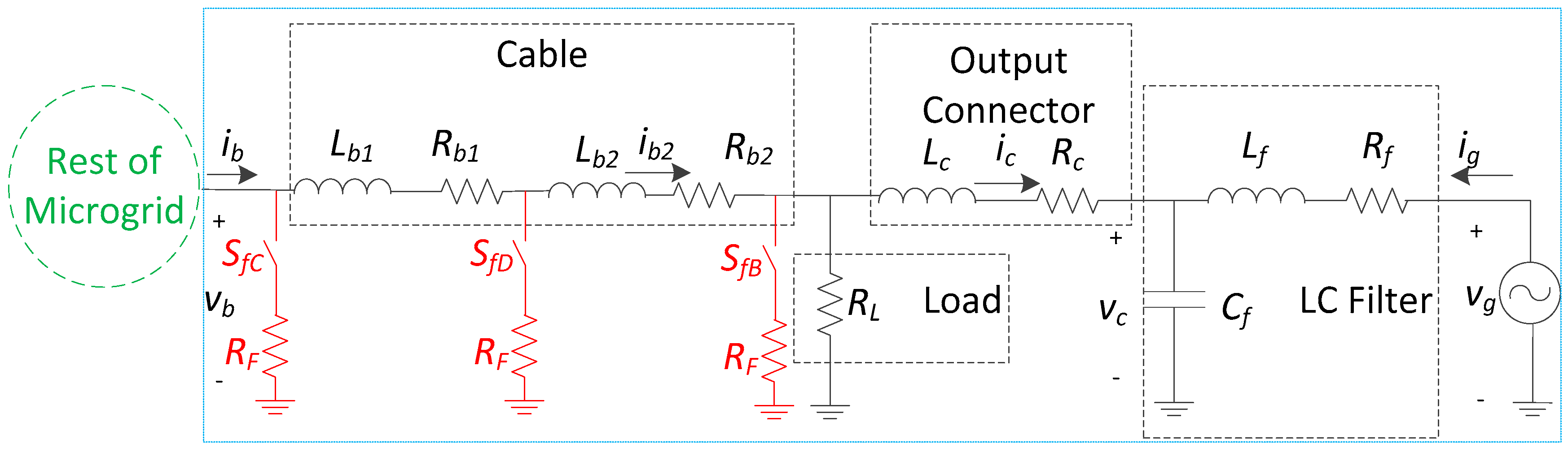
A detailed circuit representation of the microgrid feeder of
Figure 1 (components within the dotted, blue lined region) is found in
Figure 3. The fault locations under evaluation are identified in
Figure 3 and shown in red. A fault within the circuit is activated by a switch labeled
SfB,
SfC, or
SfD. To perform the aforementioned approach, the different models for the non-faulted and faulted microgrid cases are derived in the
Appendix A. These models are provided in a state-space format, from which sets of system transfer functions can be obtained, and can be used in the simulation. Three different state-space representations for various fault points within the studied microgrid and one model describing the system under normal operation are derived in the
Appendix A to show that there is a clear distinction in the matrices for faulted and non-faulted conditions.
If switch SfC is closed, this configuration corresponds to the case of a fault at the beginning of the feeder. If switch SfB is closed, this configuration corresponds to a fault near the system load. If switch SfD is closed, this configuration corresponds to a fault in the middle of the cable. Finally, if all switches are open, this case refers to normal operation of the microgrid.
Note that the system in each condition (non-faulted and faulted conditions) can be represented in the
s-domain as
where
T(
s) is the transfer function resulting from the input
vb, which can be derived by setting
ρ = 0 (see
Appendix A) and solving
where
Tg(
s) is the transfer function resulting from the input
vg. The parameters
A,
B,
C and
D are matrices corresponding to the state-space description derived in the
Appendix A. Four different transfer functions,
Tn(
s) (where
n = 1, 2, 3 and 4) are derived for the four different state space descriptions (see
Appendix A) which are used in the fault detection approach described in
Figure 2.
3. Theory/Calculation: Analytical Analysis of the Communication-Free Approach for Determining System Constraints to Avoid Nuisance Tripping and Blinding
Relying on communication is not desirable in protection systems because it degrades the reliability, slows protection operation and adds cost. This is why we investigate the effectiveness of a communication-free approach. Hence, we develop a mathematical proof showing that model-based fault detection works when only one measurement from the microgrid side is used under specific constraints.
To do so, we investigate the conditions upon which the fault identification method works when ignoring the source contribution (ig), filter and output connecter impedance at the end of the feeder. We ignore the source measurement (ig and vg) because the source and the microgrid side measurements (ib, and vb) are separated by cable with a specific length and would require the use of a communication channel to send the measurement information to the protection system if measurements on both ends are utilized. Hence, by ignoring the source, system fault identification can be communication-free. It is understood that the error between estimated system current and actual current will not be close to zero depending on the available ig. However, we propose the following:
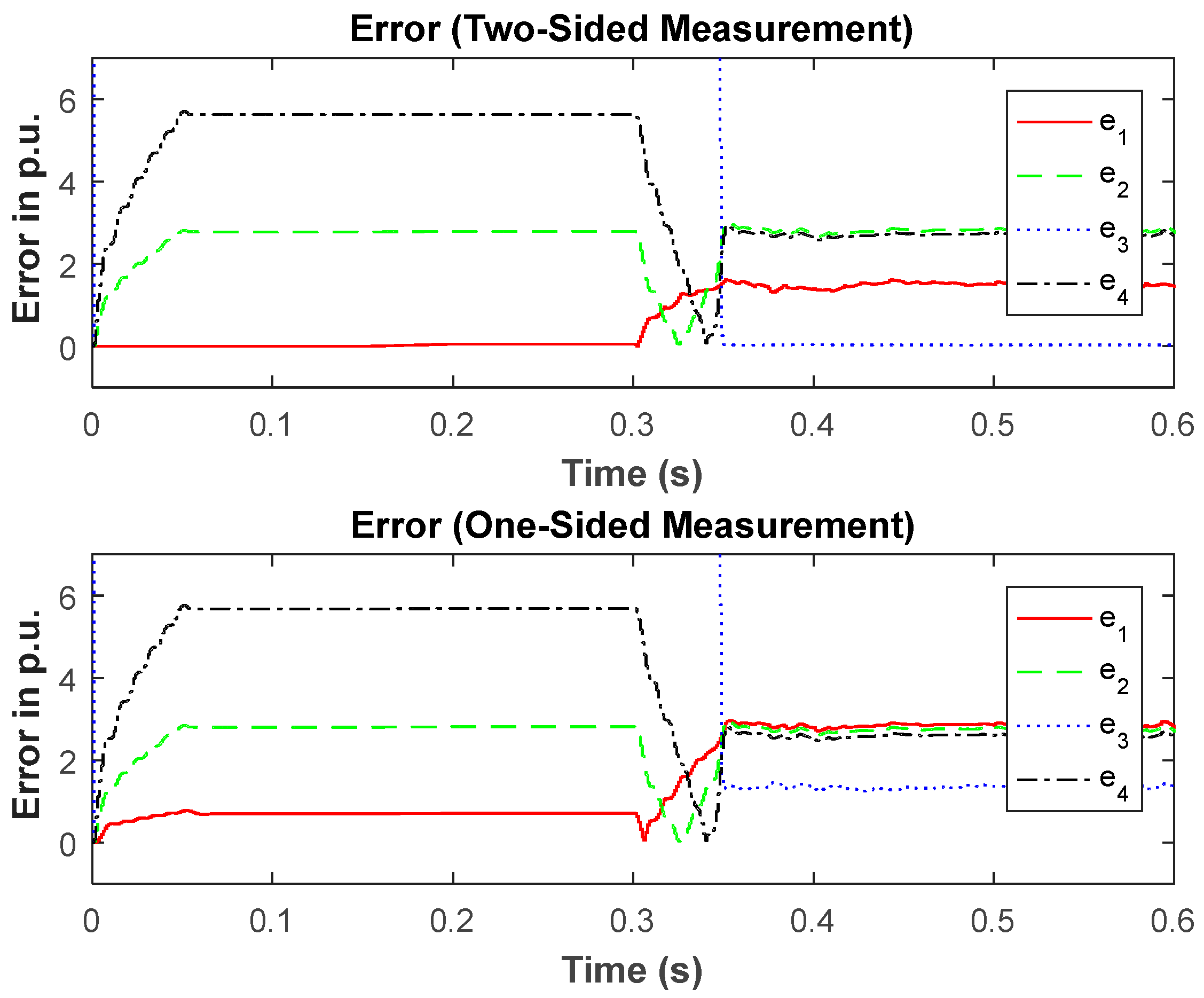
Proposition 1. The function giving the smallest error between the actual current and the estimated current describes the state of the system regardless of the size of error and regardless of the magnitude of ig for certain system constraints. This proposition is explained by the inequalities below:
- (1)
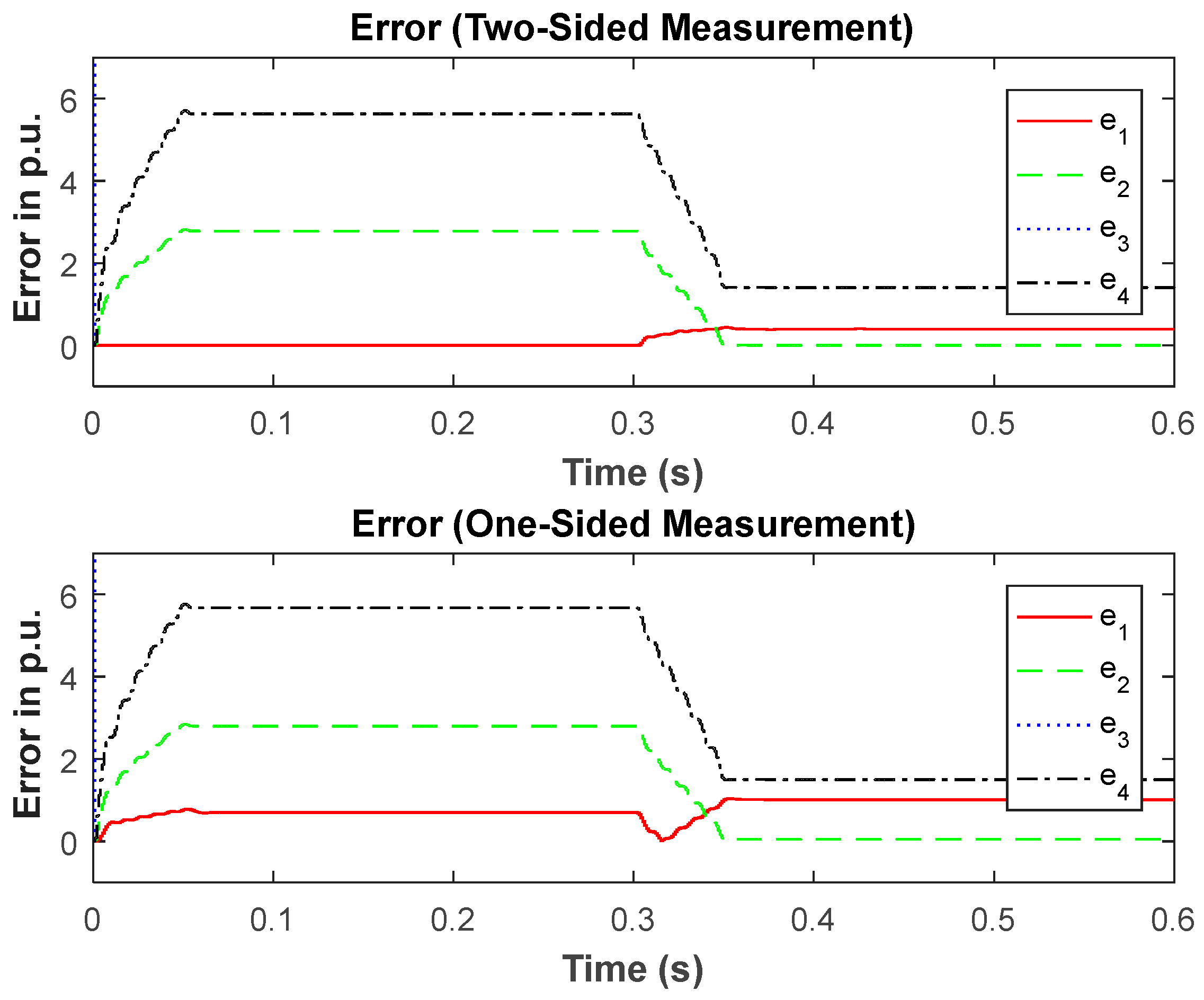
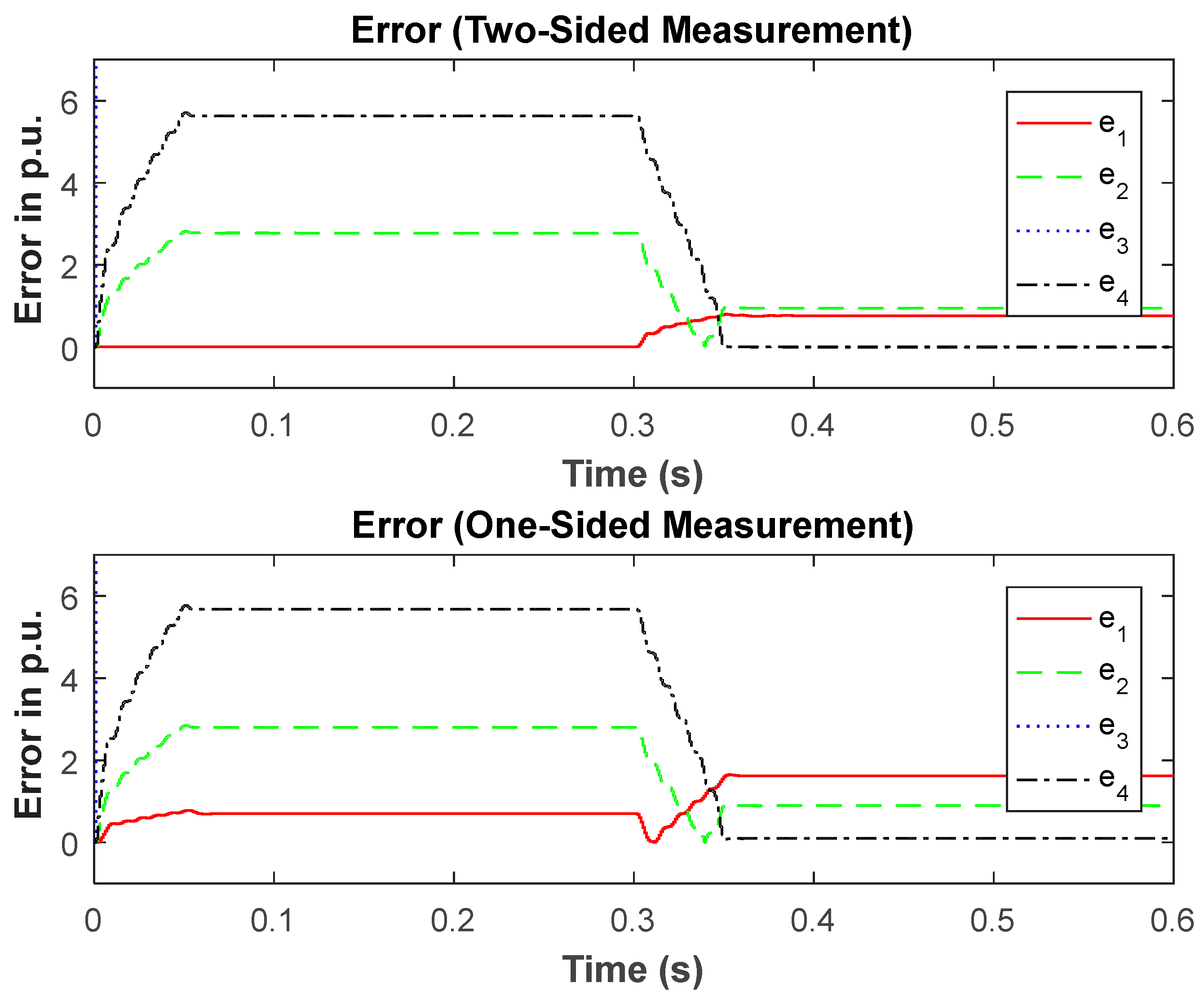
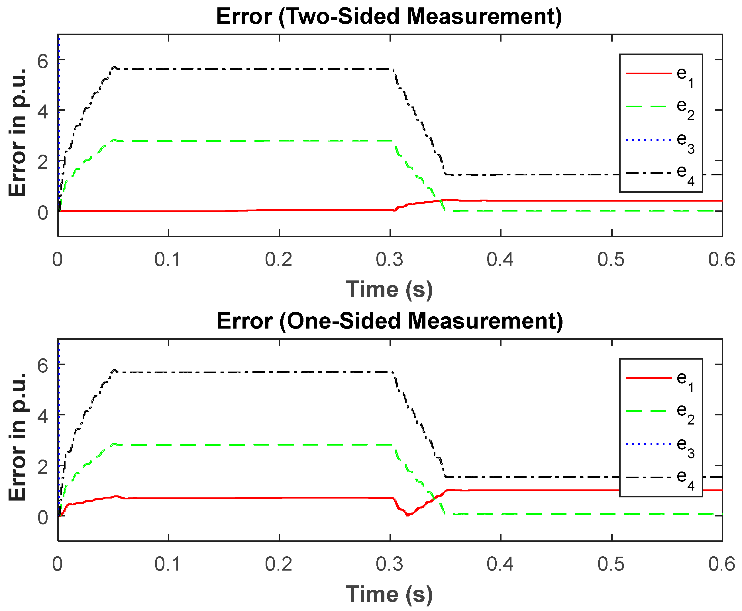
For no fault (all fault switches are opened): |e1| < |e2| and |e1| < |e3| and |e1| < |e4|
- (2)
For (SfB only closed, other switches opened): |e2| < |e1| and |e2| < |e3| and |e2| < |e4|
- (3)
For (SfC only closed, other switches opened): |e3| < |e1| and |e3| < |e2| and |e3| < |e4|
- (4)
For (SfD only closed, other switches opened): |e4| < |e1| and |e4| < |e2| and |e4| < |e3|
Note that
en is the error resulting from the difference between the measured value and the estimated output of transfer function
n which is derived from condition
n (
n = 1, 2, 3 and 4 for when all switches of
Figure 3 are open,
SfB is closed,
SfC is closed, and
SfD is closed, respectively). This error is calculated using the amplitude of the steady-state signal. In equalities 1–4 in Proposition 1 show that the error associated with the transfer function describing the true dynamics of the system
must be lower than any of the errors resulting from the remaining transfer functions with incorrect system dynamics for the given microgrid fault scenario in order to successfully detect the fault.
Before proceeding, it is important to note that according to our best knowledge the analysis in this section is a first attempt that analytically examines blinding and nuisance tripping scenarios giving clear indications of when they might occur based on system parameters. This is to allow for protection without the use of communication. Additionally, the analysis provided here presents a general guideline that can be followed to include more faulted scenarios. Hence, this analysis procedure is general enough to be easily extended to n number of faults.
Observing matrices from Equations (A3), (A7), (A8) and (A12) in the
Appendix A for the different conditions of the system, we can see that there is a clear distinction between a non-faulted condition shown in Equation (A3) and the faulted conditions shown in Equations (A7), (A8) and (A12). This will be used as a basis to detect faults in the microgrid feeder regardless of fault current levels.
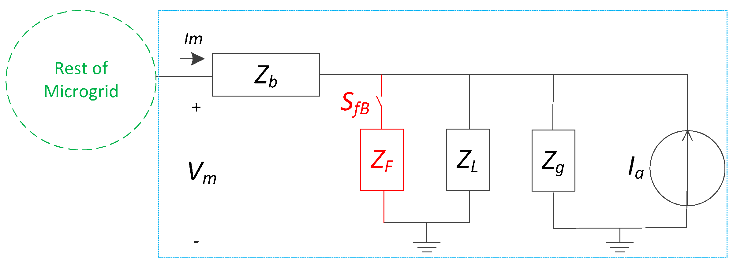
To prove Proposition 1 and find the system constraints guaranteeing its validity, we compare different mathematical relationships describing the system at different scenarios. To do so, we develop a static-based model for the non-faulted and faulted condition of the feeders as shown in
Figure 4.
Before proceeding, it is worth noting that the faulted condition used in this analysis is condition (SfB closed) only. Other conditions have not been explored because other conditions will give less restrictive constraints. The reason why condition (SfB closed) will give the most restrictive constraint is because the current contribution from the DER (ig) for other conditions (SfC closed or SfD closed) will be lower than the current for condition (SfB closed). This is because there is more impedance within the path for all faulted conditions compared to condition SfB. Additionally, the other fault conditions make a significant alteration to the state-space matrix which is evident by inspecting Equations (A3), (A8) and (A12).
Executive summary of mathematics to prove Proposition 1. Since ignoring the DER-side measurement could lead to detection errors (blinding or nuisance tripping), we investigate through counter-examples on how to avoid these errors. This is done by developing inequality constraints that guarantee the avoidance of those errors (i.e., the counter-examples of blinding and nuisance tripping). We start by assuming that the system is not-faulted and derive equations for the actual measured current (Equation (3)) and of the estimated non-faulted current based upon a one-sided measurement (Equation (4)). Then we assume that the system is faulted and derive the actual measured faulted current (Equation (5)) and the estimated fault current based upon a one-sided measurement (Equation (6)). We then develop the counter examples one by one and develop the constraints as a result of each counter example. Two different counter examples are possible. The first is for the blinding scenario and the second is for a nuisance tripping scenario. The blinding scenario occurs when the system is faulted and the detection device behaves as if the system is healthy. This occurs when the output of Equation (5) is closer in magnitude to that of Equation (4) rather than Equation (6). The nuisance tripping scenario occurs when the system is healthy and the detection device behaves as if the system is faulted. This occurs when the output of Equation (3) is closer in magnitude to that of Equation (6) rather than Equation (4). The formal mathematical relationships of these concepts are derived herewith in. The four inequality constraints listed are derived and guarantee that relay errors do not occur.
Formal mathematics to prove Proposition 1. In
Figure 4, the distributed source, filter and output connecter of
Figure 3 are lumped into the Norton equivalent represented by
Ia and
Zg. Hence, during normal operation (
Figure 4) the actual measured value of current magnitude, |
Im|, during a non-faulted condition is
where
Zb is the impedance of the line and
ZL is the load impedance. Note that
Vm,
Ia,
ZL,
Zg,
Zb, are all complex phasors. Note that the magnitude of power phasors are RMS values. In order to prove Proposition 1 and find the constraints upon which the proposition remains valid, we need to find a relationship describing the estimated current for when the current contribution (
Ia) from the distributed generation is ignored. This condition is described by (4). Equation (4) is necessary in order to construct inequalities proving Proposition 1 and the reason for its necessity will be explained in further subsections:
Here
IENF is defined as the estimate of the measured current for a non-faulted condition,
ImNF. This estimate of the non-faulted condition could be the output of the transfer function derived from Equations (A3), (A4), (A5) and (A6) if
vg is treated as a disturbance (i.e.,
ρ = 0 in the relationships found in the
Appendix A). Throughout this article, we will use the subscript
E to denote the value estimated by the model function and subscript
m to denote the actual measured value.
For the case when a fault occurs between the load and cable (
SfB closed in
Figure 4) the current magnitude representing the actual measurement is defined by
where,
Note that
Zeq is a complex phasor, and
ZF =
RF. The current estimate of the faulted condition when
SfB is closed is described by
Equations (3)–(6) will be used to prove Proposition 1 under specific system constraints. This is done by disproving all possible counter examples.
3.1. Theory/Calculation: Analytical Analysis of Masked Fault (Blinding) Scenarios
The first counter example that will be analyzed here is a masked fault scenario. A masked fault (blinding scenario) is a fault in the system that has not been detected by the proposed, communication-free detection method. When we ignore the contribution of the DER, it is possible to get a masked fault due to the effects of the DER because the DER produces current that we are not accounting for. A masked fault occurs when
while the system is faulted. This scenario occurs when inequality Equation (7) is satisfied:
Inequality Equation (7) describes a condition when there is a fault in the system yet the model for the non-faulted case gives a smaller error than the model for the faulted case when compared to actual measurement. This leads to a masked fault condition. Solving Equation (7) gives four distinct regions depending on the left hand side (LHS) and right hand side (RHS) sign of the expressions within the outside absolute value of Equation (7) ( and ). The four distinct region analyses are as follows:
• If LHS ≥ 0 and RHS ≥ 0
Here Equation (7) becomes
Solving Equation (8) gives
Note the real and imaginary parts of
Zb,
ZL and
ZF are positive. Therefore, Equation (9) is satisfied when Equation (10) is satisfied.
Inequality Equation (10) can never be satisfied implying that Equation (9) is never satisfied. Thus, Equation (8) is never satisfied. Hence, a masked fault never occurs within this region.
• If LHS < 0 and RHS < 0
Here Equation (7) becomes
Inequality Equation (11) is always satisfied because Equation (8) is never satisfied. Therefore, in order to know the conditions of the system giving a masked fault, we check the bounds of this region which is defined by (
LHS < 0 and
RHS < 0) as
If one of the sides of Equation (12) is dissatisfied then we are guaranteed that Equation (12) is never satisfied because the two sides of Equation (12) have to be satisfied simultaneously. Hence, we only investigate
LHS < 0 which is
Realize that
Vm, and
Ia are complex quantities, and |
Im| is a the
RMS signal. Substituting Equation (4) and Equation (5) into Equation (13), simplifying and rearranging gives
Our ultimate goal is to disprove all counterexamples or give as few and as relaxed constraints as possible to disprove all counterexamples. For the case if either side of Equation (12) is prevented from being true (never operating in this region), we can guarantee that a masked fault never occurs. Hence, inequality Equation (13) can be made to always be false so that Equation (12) is never satisfied. This is done by performing an inequality reversal to force the system to always operate in the opposite region. Hence, the sign of Equation (14) is redirected and we solve for an impedance ratio limit which is shown as Constraint 1:
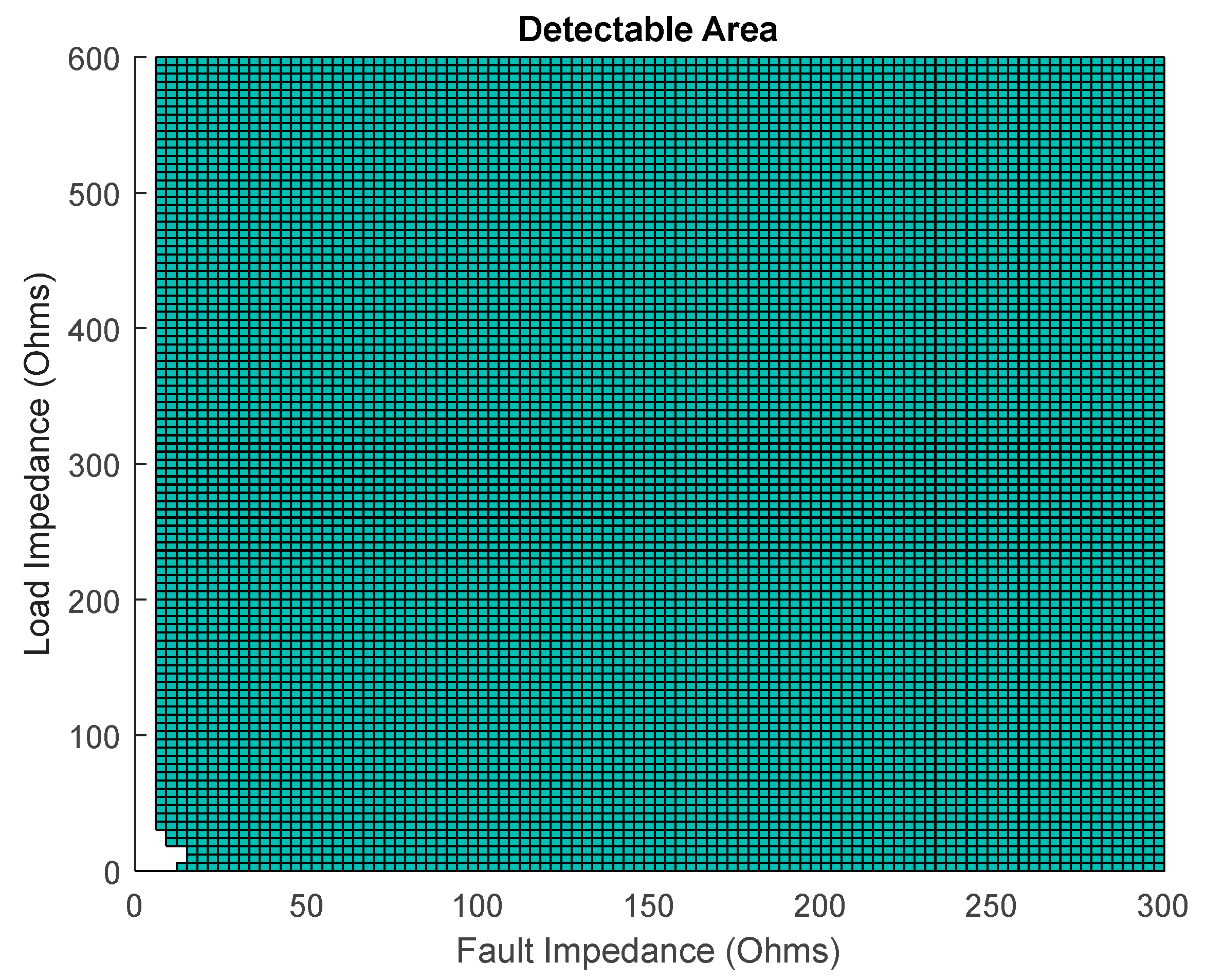
Constraint 1: The inequality below must be satisfied to prevent a masked fault scenario: Note that backup protection based on low-voltage (lower than IEEE1547 ride-through requirements) is assumed to always exist. Hence, Vm in Constraint 1 is a constant quantity chosen above the backup protection value. Current Ia should be as large as possible during faulted conditions which is typically 2 p.u. for inverters. Analyzing the microgrid according to Equation (15), the range of fault impedances (ZF) that the apparatus can detect can be determined. The constraint should be tested for the minimum and maximum possible values of ZL. Constraint 1 represented by Equation (15) provides the following physical insight: the ratio of the faulted system equivalent impedance to the non-faulted system equivalent impedance must be lower than the ratio of the voltage drop across the cable up to the fault point to the total voltage (Vm).
• If LHS ≥ 0 and RHS < 0
Here Equation (7) becomes
Solving Equation (16) does not give much physical insight. Hence, we reverse the inequality sign of Equation (16) so that it is never satisfied and find a system constraint preventing a masked fault:
Constraint 2: The inequality below must be satisfied to prevent a masked fault scenario: Note that the result of ZF based on Constraint 1 can be substituted into Constraint 2 to make sure that Equation (17) is true. If it is not, then ZF is lowered and the analysis process is repeated until Equation (17) is satisfied. At the end of the iterations, the maximum value of ZF that the communication-free method can detect will be obtained. An optimization problem can also be formulated to find the optimal values.
• If LHS < 0 and RHS ≥ 0
Here Equation (7) becomes
Solving Equation (18) for when
ZF = 0 Ω gives us a condition where it is always satisfied. Therefore, we check the system parameters that allow the system to operate in this region if this region exists for a general
ZF (all possible types of faults—low and high impedance). This region (
LHS < 0 and
RHS ≥ 0) is expressed by
By examining Equation (19), we see that the left hand side of this equation is the same as Equation (13). Equation (13) is forced to always be false by Constraint 1. Hence, Equation (19) cannot be satisfied under Constraint 1. Therefore, a masked fault is impossible for this region.
3.2. Theory/Calculation: Analytical Analysis of False Positive (Nuisance Tripping) Scenarios
The only other counterexample that must be disproven to prove Proposition 1 to find all the constraints that guarantee its validity is a false positive (nuisance trip) scenario. A false positive scenario occurs when there is no fault and we falsely identify a fault (i.e., when
while there is no fault). This condition occurs when the following is satisfied:
Here, the LHS and RHS are redefined to be the expressions within the outside absolute value of (20) (i.e., and ). Solving Equation (20) gives four distinct regions as follows:
• If LHS ≥ 0 and RHS ≥ 0
Here Equation (20) becomes
Solving Equation (21) gives
Equation (22) is the same as Equation (9) but with a reversed inequality sign and we concluded that Equation (9) can never be satisfied. Hence, Equation (22) is always satisfied. Therefore, if this region is entered, there is always a false positive. Hence, we check if it is possible to operate in this region or find the conditions that make the system operate within these boundaries. This region is expressed by
Solving
LHS ≥ 0 of (23), we obtain
where,
Equation (24) does not give much insight as to whether or not it is possible to operate in this region. Hence, we reverse the inequality sign of Equation (24) so that Equation (24) is never satisfied and find a system constraint (Constraint 3) preventing a false positive. Note that in forthcoming section when we solve for the maximum value of
ZF, this gives us the value of the highest impedance for a fault on the system, which the apparatus can detect. However, in this section the analysis is for a false positive scenario, which means that there is no fault to begin with. Hence, the constraints here restrict the value of the assumed fault impedance in the model equations. However, when the range of the assumed fault resistance is decreased, this also decreases the range of faults that can be detected when faults occur. Hence, a trade-off between protection system dependability (guaranteeing the relay always operates for faults) and security (guaranteeing the relay will not trip when there is no fault) is made. In protection system design, this trade-off always exists [
31] and the same is true for the proposed method. From Constraint 3, to make the protection system more secure, the fault impedance used in the model equations needs to be lowered. However, the more this impedance is lowered, the lower the range of fault impedances that can be detected in the communication-free approach (more security as opposed to more dependability). Hence, a thorough analysis has to be done by the designer to choose whether dependability versus security is valued most for a particular application. It is worth noting here that the communication-based approach is more robust in detecting a wide range of faults with a higher range of fault impedance.
Constraint 3: The fault impedance value used to calculate the equations must be such that the system satisfies the following constraint if security is desired over dependability: Note that here
Vm is chosen (for
Section 3.2 constraints) based on the largest possible stable normal operating value (i.e.,
Vm = 1.10 p.u.) as opposed to the smallest possible faulted value for
Section 3.1 constraints. This is because a nuisance trip means that we are operating normally as opposed to a faulted condition in a blinding scenario in
Section 3.1. Also, the constraint is checked for the largest and smallest possible
Ia and
ZL during normal operation.
• If LHS < 0 and RHS < 0
Inequality (28) is the same as (9) which was proven to never be satisfied in
Section 3.1. Hence, (27) is never satisfied and a false positive can never occur in this region.
• If LHS ≥ 0 and RHS < 0
In region (LHS ≥ 0 and RHS ≥ 0) Constraint 3 has already been derived to prevent LHS ≥ 0 from occurring. This means we can never operate in this region under Constraint 3. Hence, a false positive can never occur in this region.
• If LHS < 0 and RHS ≥ 0
Here Equation (20) becomes
Solving Equation (29) yields
Inspecting Equation (30) does not provide much insight into a system physical constraint. Hence, we investigate the region (LHS < 0 and RHS ≥ 0) to get insight into the possibility of a false positive.
First,
LHS < 0 is solved to obtain
Then,
RHS ≥ 0 is solved to achieve
Here, we try to use all possible Equations (30)–(32) to give multiple sufficient conditions guaranteeing the prevention of a false positive. We do this to give more room for ZF to increase in order to increase dependability while keeping the same level of security.
If one of the inequalities of Equations (30), (31) or (32) is reversed then a false positive can never occur. However, Equation (31) cannot be reversed to prevent a false positive because that will violate Constraint 3 developed in Equation (26). Hence, the system must satisfy one of the equations listed as Constraint 4.
Constraint 4: One of the following conditions must be satisfied to prevent a false positive if security is desired over dependability: Note that the values derived from the previous constraints (Constraints 1–3) are checked against Constraint 4. If Constraint 4 is satisfied, then the analysis procedure ends. If it is not, then the analysis is repeated until all constraints are satisfied.
5. Discussion
Selecting an appropriate protection scheme for a microgrid design is dependent upon available capital, engineering requirements, and system topology. To compare the model-based approach developed in this work, a qualitatively summary of common relay protection techniques with specific benchmark features is outlined in
Table 1. Overcurrent, symmetrical component, overvoltage, differential and distance protection schemes are the common routines that are well developed. Adaptive and traveling wave methods have shown promise by various research groups and in test settings. The phase-based and model-based approaches are beginning to be conceptualized and evaluated by the engineering community.
With microgrids in mind, the top criteria is understanding if a communication system is required and how robust a protection scheme must be for the distributed loads throughout the system architecture. An interesting observation is that these two criteria often go hand-in-hand, that is, if a communication system exists then the specific method will be robust against distributed loads impacting fault identification. An advantage is shown in that the model-based approach does not require a communication system but is robust enough to identify faults in the presence of distributed load.
The methods requiring communication include differential, adaptive, traveling wave, and PMU approaches. Only the adaptive, traveling wave, and PMU have the required robustness for distributed load but come at a higher cost due to processing power in the hardware. An advantage is found in model-based approaches as they will be cheaper because they require no communication system and are robust against distributed load and varying network impedance as shown in the results section.
Regarding sensing technology, the methods can be ranked. Traveling wave approaches use current sensors, which are a well defined technology. Phase based approaches will need to measure both voltage and current to measure the phase differential changes, which is slightly more challenging than the latter. The model-based work used in this work utilized and understanding of system impedances. An argument can be made that impedance measurement can be challenging to quantify, however, all microgrids are all custom designed and smaller in scale compared to bulk power systems such that the microgrid impedances can be estimated with strong accuracy. Therefore, the model-based approach sensing technology technique becomes comparable to the phase-based approach but the former has higher robustness to fault identification. Adaptive routines use current sensing but the routines require a lot of processing power with the amount of information obtained from the system.
The largest competition for the model-based approach developed in this work are the traveling wave approaches in the context of microgrid design, robustness to distributed loads, sensing technology and cost. However, the main differentiator between both besides cost is the ability to identify blinding and nuisance tripping scenarios. Traveling wave based relay settings require precise tuning for sensitivity reasons and can lead to nuisance tripping. The impedance based constraints for blinding and nuisance tripping scenarios for the model-based approach in this paper have been derived and can be derived similarly for other architectures to ensure blinding and nuisance tripping will not occur. Blinding and nuisance tripping for the advanced, communication based approaches are not analyzed in the literature according to the author’s knowledge.
This article provided models for different conditions (faulted and non-faulted) for a microgrid feeder. These models were developed and to be used in a model-based approach to detect faults in the case of low-fault current levels in inverter-dominated microgrids. To make the system more reliable, faults can be detected without introducing communication; a mathematical proof and system constraints are provided. The method developed in the article can easily distinguish between non-faulted and faulted conditions of microgrids regardless of fault current levels because faults cause significant alterations to the governing system relationships. The proposed approach can be extended to other microgrid configurations. The faults are detected in steady-state here. However, the models developed in the
Appendix A can serve as a basis to develop future methods that operate much faster by investigating the transient region for the model-based fault detection. Additionally, the approach that we followed to derive system constraints provides a general framework that can be applied to other protection methods to avoid nuisance tripping and blinding scenarios. This framework also serves as a general foundation to study DER effects on systems and perform inverter-based system design more effectively.


