An Improved Multi-Timescale Coordinated Control Strategy for Stand-Alone Microgrid with Hybrid Energy Storage System

Abstract

A scientific and effective coordinated control strategy is crucial to the safe and economic operation of a microgrid (MG). With the continuous improvement of the renewable energy source (RES) penetration rate in MG, the randomness and intermittency of its output lead to the increasing regulation pressure of the conventional controllable units, the increase of the operating risk of MG and the difficulty in improving the operational economy. To solve the mentioned problems and take advantage of hybrid energy storage system (HESS), this study proposes a multi-time scale coordinated control scheme of “day-ahead optimization (DAO) + intraday rolling (IDR) + quasi-real-time correction (QRTC) + real-time coordinated control (RTCC).” Considering the shortcomings of existing low prediction accuracy of distributed RES and loads, the soft constraints such as unit commitment scheduling errors and load switching scheduling errors are introduced in the intraday rolling model, allowing the correction of day-ahead unit commitment and load switching schedule. In the quasi-real-time coordinated control, an integrated criterion is introduced to decide the adjustment priority of the distributed generations. In the real-time coordinated control, the HESS adopts an improved first order low pass filtering algorithm to adaptively compensate the second-level unbalanced power. Compared with the traditional coordinated control strategy, the proposed improved model has the advantages of good robustness and fast solving speed and provides some guidance for the intelligent solution for stable and economic operation of stand-alone MG with HESS.

1. Introduction

In recent years, distributed generation (DG) technology has rapidly developed due to its advantage of efficiently consuming energy locally. To fully take advantage of DG and improve the safety and reliability of power supply, the MG is proposed as an effective scheme to improve the DG penetration rate of the distribution network.

MG consists of distributed generations (DGs), energy storage system (ESS), power load, monitoring, protection and automation devices. It can be viewed as a small power supply system that can realize the internal power balance. MG can operate in many modes. It can connect to the distribution network through point of common coupling (PCC), operating as an “equivalent controllable load.” Or it can be disconnected from the distribution network operating in stand-alone mode and provides power for the interior load [1,2]. For occasions where it is not feasible to establish distribution network, MG can only operate independently and autonomously [3,4,5,6]. For the stand-alone MG, the current mainstream operation control strategies are master-slave strategy and peer-to-peer strategy [7]. In master-slave strategy, one of the DGs (diesel generators, PV system, ESS, etc.) uses V/f control method, producing voltage and frequency references for other DGs and other DGs use P/Q control method. While in peer-to-peer strategy, each DG that participates in V/f regulation and control plays an equivalent role. In this strategy, DG controllers usually use droop control, automatically dispatch the output power.

A scientific and effective coordinated control strategy is crucial to the safe and economic operation of MG. Current researches on coordinated control of stand-alone MGs can be categorized into two groups: coordinated control strategies based on fixed logic criteria and strategies based on optimization theory. Reference [8] targets at stand-alone MG that contains wind turbine (WT), photovoltaic (PV) system, diesel generators (DSGs) and ESS and summarizes several commonly used coordinated control strategies based on logic criteria, including power smoothing strategy, minimum running time strategy for DSGs, soft cycle charging strategy, hard cycle charging strategy and so forth. Since the fixed logic criteria based control strategy is based on pre-analysis and operational experience and does not change with the load or RES, it is easy to design and has high decision-making speed. Therefore, most of the stand-alone MGs adopt this kind of strategy.

Due to the volatility and randomness of RES, the fixed logic criteria based coordinated control strategy cannot guarantee optimal economic operation of MG. Therefore, the strategy based on optimization theory has been extensively studied by scholars. An improved simplified warm optimization method for day-ahead operation optimization model is proposed in [9]. The day-ahead model includes fuel cost, battery operation cost and power transmission cost. In [8], an economic dispatch model considering battery lifetime for MG is proposed. A scenario-based robust energy management method accounting for the worst-case amount of renewable generation (RG) and load is developed in [10]. Reference [11] presented an optimal management of battery energy storage in a PV-based commercial building to increase its resilience as it minimizes its operational cost. The Conditional Value at Risk (CVaR) was used to account for the uncertainties in both the day-ahead electricity price and the PV power generation. To deal with the prediction uncertainties of RE and loads and take advantage of the time-of-use electricity price, reference [12] developed an interval-based optimization model for maximum profits.

The above papers are based on day-ahead prediction results, focusing on the research of day-ahead scheduling optimization model to reduce the risk brought by the uncertainty of RES. However, compared to centralized RES, the prediction accuracy of distributed RES is poor, so the schedule result may not be directly applied in MG. Reference [13] shows that the shorter the prediction horizon, the higher the prediction accuracy. So, the using of control strategy with smaller timescale can correct the residual errors produced in larger timescale. Therefore, ultra-short-term prediction with smaller timescale is applied to the IDR optimization in MG and multi-timescale coordinated control strategies have emerged. Reference [14] developed an energy management framework for MG including multi-timescale demand response. The timescales are days, hours and minutes. The hour-ahead scheduling model is based on model prediction control, with prediction data generated by ultra-short-term prediction. Reference [15] proposes a coordinated control strategy in day-ahead and intraday aspects, considering battery lifetime degradation cost when optimizes operation cost. In [14,15], the startup and shutdown schedule of controllable generation units cannot be modified. When the day-ahead prediction error is high, it is possible that the generation power cannot balance load power. [16] proposes a two-timescales robust optimization method by scheduling energy storage and the direct load control. Reference [17] proposed an energy management model for MG based on day-ahead and real-time timescale. Day-ahead power prediction is used in the decision-making of next-day economic operation of MG. A fuzzy control based supervisory control strategy is adopted in real-time timescale to reduce the tie line power deviation. In [18], a strategy for obtaining optimal scheduling of multiple microgrid systems with power sharing through coordination among microgrids that have no cost function of generation units is proposed.

However, these papers have the following shortcomings:

(1)

HESS is not included as an element of coordinated control; thus, applicability is limited.

(2)

The SOC balance of HESS in daily dispatch period has not received enough attention.

(3)

The multi-timescale framework is relatively simple, with large gap between different timescales.

At present, energy-type ESS (ETESS) such as batteries are usually used as the main energy storage device in MG. ETESS has the characteristics of high energy density, low power density, short cycle life and slow power response, thus cannot economically smooth high frequency disturbance in MG. Power-type ESS (PTESS) represented by supercapacitor (SC) has the characteristics of high power density, low energy density, long cycle life and fast power response. Therefore, a better solution is to combine ETESS and PTESS, forming HESS. According to [5], it is proved theoretically that HESS can make full use of the complementary advantages of battery and SC, improve the output performance of ESS and prolong the service life of battery, reducing the life cycle cost of ESS. By now, many research has been conducted on the optimal configuration and control methods for HESS [19,20,21] but only a few research on energy management and coordinated control for MG wit HESS. Reference [22] proposed a two-layer energy management framework for HESS composed of battery and SC and incorporated the battery cycle charge and discharge life loss into the model. However, this study is only for MG with RES, HESS and load, limited for the scenario where other controllable power sources (for example, diesel generators and micro gas turbine) exist in MG. Reference [23] proposed a two-layer energy scheduling framework for MG: hour-ahead scheduling and real-time scheduling. In hour-ahead scheduling, a deterministic optimization model is formulated to minimize the operation cost of microgrids and to guarantee the operation safety. The real-time scheduling is conducted every minute and the scheduling period is still too long compared to the SC with a charge and discharge cycle of only tens of seconds.

In this paper, an improved multi-time scale coordinated control strategy is proposed for stand-alone MG with HESS. The strategy consists of day-ahead optimization model, model predictive control based intraday rolling optimization model, comprehensive criteria based quasi-real-time correction model and real-time coordinated control model. Compared with the traditional coordinated control strategy, the proposed improved model has the advantages of good robustness and fast solving speed and provides some guidance for the intelligent solution for stable and economic operation of stand-alone MG with HESS.

The remainder of this paper is organized as follows. Section 2 describes the typical topology of stand-alone microgrid with hybrid energy storage system. Section 3 presents the multi-time scale coordinated control proposed in this paper. Section 4 demonstrates and analyzes the simulation results of a case study. Summary, conclusions and outlook are given in Section 5.

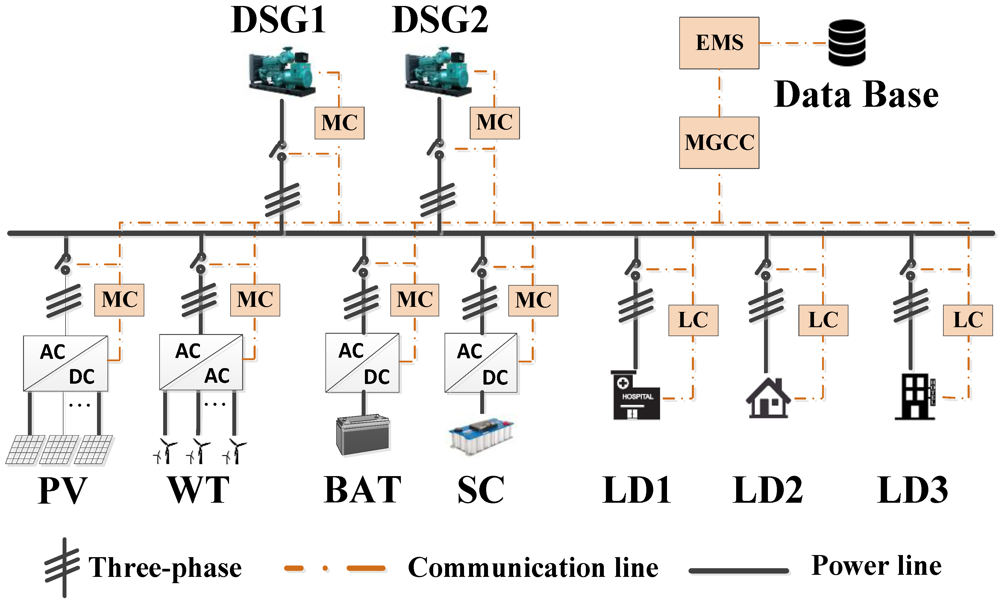
2. Typical Topology of Stand-Alone Microgrid with Hybrid Energy Storage System

Figure 1 is a typical topology of stand-alone MG with HESS. In this MG, wind power generation units, PV units, diesel generation units, HESS and load are connected to the AC bus through multiple feeders. Feeders are usually equipped with circuit breaker and the entire grid has a radial structure.

The hierarchical control architecture is adopted to allocate the secondary system of stand-alone MG and each layer has a corresponding control unit to execute the control strategy:

(1)

The first layer is the optimal schedule layer and the corresponding control unit is EMS (energy management system). The DAO and IDR algorithm in EMS is used to realize coordinated control strategy of a large time scale and provide scheduling curve for MGCC (microgrid central controller).

(2)

The second layer is the MG control layer and the corresponding control unit is MGCC. The QRTC and RTCC in MGCC based on logical judgment is used to correct the deviation between the actual operating state and the ideal state of the MG and issue control commands to the device controller.

(3)

The third layer is the local control layer and the corresponding control unit is device controllers. Control commands from the MG real-time control layer are executed by DGs/load/HESS.

To coordinate various DGs in MG, it is necessary to model the operating characteristics and boundaries of DGs, including the wind power system operation model, PV power system operation model, diesel power generation system operation model, the charge/discharge model of HESS and energy storage life model and so forth. The wind power and PV power system operation model re implemented by [18], the diesel model is implemented by [15], the HESS model is implemented by [24,25] and the life model is implemented by [26]. These models will not be further discussed here.

3. Multi-time Scale Coordinated Control

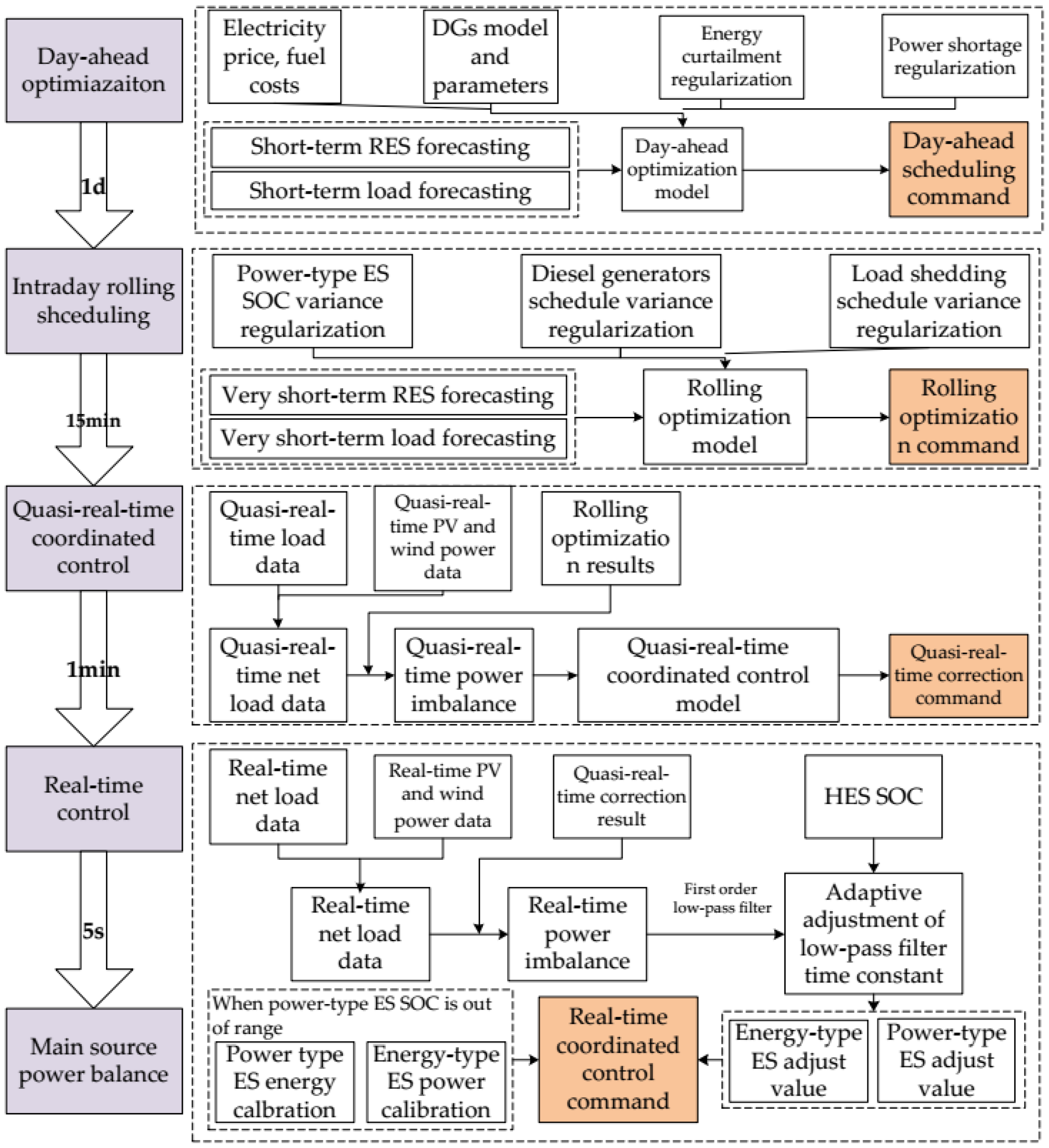
3.1. Multi-time Scale Coordinated Control Framework

The framework of multi-time scale coordinated control is shown in Figure 2. This framework is comprised of day-ahead optimization model, intraday rolling scheduling model, quasi-real-time coordinated control model and real-time control model, which are described as follows:

(1)

Day-ahead optimization model: Based on the short-term load forecasting results, DGs’ hourly output scheduling curve (except PTESS) and load switching scheme are determined by DAO Day-ahead optimization model in the EMS. The execution cycle of this model is 1 day.

(2)

Intraday rolling model: Based on the ultra short-term power forecasting results, the DAO results are continuously corrected by the time-limited rolling optimization scheduling. The time scale of the rolling time window is 4h (same as the ultra short-term prediction). The model has an execution cycle of 15 min.

(3)

Quasi-real-time coordinated control model: The deviation between the constantly updated intraday rolling scheduling plan and the actual operating conditions of MG is calculated by the real-time collected data and will be corrected quickly. An integrated criterion is introduced to decide the adjustment priority of the distributed generations. The execution cycle of this model is 1 min.

(4)

Real-time coordinated control model: Under the condition of ensuring frequency and voltage stability, real-time control commands are determined to follow the command from quasi-real-time coordinated control as much as possible in second time scale and real-time smooth control strategy for HESS based on logic judgment is used to smooth unbalanced power of second time scale. The execution cycle of this model is 5 s.

3.2. Day-Ahead Optimization Model

3.2.1. Decision Variables

This paper assume that stand-alone MG includes WT system, PV system, ETESS, PTESS and DSGs on the source side and important load, secondary load and interruptible load of participation in demand response on the load side. The optimization variables of the MG’s day-ahead optimization scheduling model include the set P of output scheduling curves of controllable DGs and the set u of DG unit commitment and load switching schedule:

$$\begin{array}{l}\mathit{P}=\left\{{\mathit{P}}_{\mathrm{de},i},{\mathit{P}}_{\mathrm{ba},j},{\mathit{P}}_{\mathrm{pv},l},{\mathit{P}}_{\mathrm{wt},m}\right\};\mathit{u}=\left\{{\mathit{u}}_{\mathrm{de},i},{\mathit{u}}_{\mathrm{ba},j},{\mathit{u}}_{\mathrm{sdload},k},{\mathit{u}}_{\mathrm{itload},p}\right\}\\ \{\begin{array}{l}{\mathit{P}}_{\mathrm{de}}=\left\{{\mathit{P}}_{\mathrm{de},1},{\mathit{P}}_{\mathrm{de},2},\cdots ,{\mathit{P}}_{\mathrm{de},i},\cdots ,{\mathit{P}}_{\mathrm{de},n_{\mathrm{de}}}\right\}\\ {\mathit{P}}_{\mathrm{ba}}=\left\{{\mathit{P}}_{\mathrm{ba},1},{\mathit{P}}_{\mathrm{ba},2},\cdots ,{\mathit{P}}_{\mathrm{ba},j},\cdots ,{\mathit{P}}_{\mathrm{ba},n_{\mathrm{ba}}}\right\}\\ {\mathit{P}}_{\mathrm{pv}}=\left\{{\mathit{P}}_{\mathrm{pv},1},{\mathit{P}}_{\mathrm{pv},2},\cdots ,{\mathit{P}}_{\mathrm{pv},l},\cdots ,{\mathit{P}}_{\mathrm{pv},n_{\mathrm{pv}}}\right\}\\ {\mathit{P}}_{\mathrm{wt}}=\left\{{\mathit{P}}_{\mathrm{wt},1},{\mathit{P}}_{\mathrm{wt},2},\cdots ,{\mathit{P}}_{\mathrm{wt},m},\cdots ,{\mathit{P}}_{\mathrm{wt},n_{\mathrm{wt}}}\right\}\\ {\mathit{u}}_{\mathrm{de}}=\left\{{\mathit{u}}_{\mathrm{de},1},{\mathit{u}}_{\mathrm{de},2},\cdots {\mathit{u}}_{\mathrm{de},k},\cdots ,{\mathit{u}}_{\mathrm{de},n_{\mathrm{de}}}\right\}\\ {\mathit{u}}_{\mathrm{ba}}=\left\{{\mathit{u}}_{\mathrm{ba},1},{\mathit{u}}_{\mathrm{ba},2},\cdots ,{\mathit{u}}_{\mathrm{ba},j},\cdots ,{\mathit{u}}_{\mathrm{ba},n_{\mathrm{ba}}}\right\}\\ {\mathit{u}}_{\mathrm{sdload}}=\left\{{\mathit{u}}_{\mathrm{sdload},1},{\mathit{u}}_{\mathrm{sdload},2},\cdots ,{\mathit{u}}_{\mathrm{sdload},k},\cdots ,{\mathit{u}}_{\mathrm{sdload},n_{\mathrm{sdload}}}\right\}\\ {\mathit{u}}_{\mathrm{itload}}=\left\{{\mathit{u}}_{\mathrm{itload},1},{\mathit{u}}_{\mathrm{itload},2},\cdots ,{\mathit{u}}_{\mathrm{itload},p},\cdots ,{\mathit{u}}_{\mathrm{itload},n_{\mathrm{itload}}}\right\}\end{array}\end{array}$$

(1)

where $n_{\mathrm{de}}$, $n_{\mathrm{ba}}$, $n_{\mathrm{pv}}$, $n_{\mathrm{wt}}$, $n_{\mathrm{sdload}}$, $n_{\mathrm{itload}}$ are the number of diesel generators, ETESS, PV system, wind power system, secondary load and interruptible load. ${\mathit{P}}_{\mathrm{de}}$, ${\mathit{P}}_{\mathrm{ba}}$, ${\mathit{P}}_{\mathrm{pv}}$, ${\mathit{P}}_{\mathrm{wt}}$ are the output schedule matrix of diesel generators, ETESS, PV system and wind power system. ${\mathit{u}}_{\mathrm{de}}$, ${\mathit{u}}_{\mathrm{ba}}$ are the operation state matrix of diesel generators and ETESS, where 0 means stopped and 1 means running. ${\mathit{u}}_{\mathrm{sdload}}$, ${\mathit{u}}_{\mathrm{ctload}}$ are load switching schedule matrix of secondary load and interruptible load, where 0 means off and 1 means on. ${\mathit{P}}_{\mathrm{de},i}$ is the output schedule of the ith diesel generator for the next 24 h. ${\mathit{P}}_{\mathrm{ba},j}$ is the charging/discharging schedule of the jth ETESS for the next 24 hours. ${\mathit{P}}_{\mathrm{pv},l}$ is the output schedule of the lth PV system for the next 24 h. ${\mathit{P}}_{\mathrm{wt},m}$ is the output schedule of the mth wind power system for the next 24 h. ${\mathit{u}}_{\mathrm{de},i}$ is the unit commitment of the ith diesel generator for the next 24 h. ${\mathit{u}}_{\mathrm{ba},j}$ is the unit commitment of the jth ETESS for the next 24 h. ${\mathit{u}}_{\mathrm{sdload},k}$ is the load switching schedule of the kth secondary load. ${\mathit{u}}_{\mathrm{ctload},p}$ is the load switching schedule of the pth interruptible load.

Since the time scale of PTESS’s charge-discharge cycling is second and charge-discharge capacity is very small, there is no need to optimize the output scheduling of PTESS in day-ahead optimization.

3.2.2. Objective Function and Constraints

To maximize the utilization of RES under the condition of ensuring MG safety and stability and maintain system reliability, the objective function consist of operation cost F and decision penalty term C. The operation cost includes diesel generators operation cost, ETESS cost, RES system cost and load profit (electricity selling profit and interruptible load compensation). The decision penalty term includes penalty of abandoned solar and wind power and load outage. Since the objective function includes the penalty term above, the system will make the decisions of RES curtailment or load shedding only when the safety and stability constraints cannot be satisfied. Considering system power balance constraint, reserve capacity constraint and operation constraints of each DGs, a day-ahead optimization model of stand-alone MG is established as follows:

$$\begin{array}{cc}\hfill y(\mathit{P},\mathit{u})& =F_{\mathrm{load}}({\mathit{u}}_{\mathrm{load}})-F_{\mathrm{ba}}({\mathit{P}}_{\mathrm{ba}},{\mathit{u}}_{\mathrm{ba}})-F_{\mathrm{de}}({\mathit{P}}_{\mathrm{de}},{\mathit{u}}_{\mathrm{de}})-F_{\mathrm{re}}({\mathit{P}}_{\mathrm{pv}},{\mathit{P}}_{\mathrm{wt}})\hfill \\ & +C_{\mathrm{dep}}({\mathit{P}}_{\mathrm{pv}},{\mathit{P}}_{\mathrm{wt}})+C_{\mathrm{lpsp}}({\mathit{u}}_{\mathrm{load}})\hfill \end{array}$$

(2)

$$F_{\mathrm{de}}={\displaystyle \sum _{t=1}^{T_1}{\displaystyle \sum _{i=1}^{n_{\mathrm{de}}}\begin{array}{l}[(s_{\mathrm{de},\mathrm{start},i}(t)f_{\mathrm{de},\mathrm{start}}+s_{\mathrm{de},\mathrm{down},i}(t)f_{\mathrm{de},\mathrm{down}})+\\ f_{\mathrm{diesel}}(P_{\mathrm{de},i}\Delta T)+g_{\mathrm{diesel}}(P_{\mathrm{de},i}\Delta T)]\end{array}}}$$

(3)

$$F_{\mathrm{ba}}={\displaystyle \sum _{t=1}^{T_1}{\displaystyle \sum _{j=1}^{n_{\mathrm{ba}}}{f}_{\mathrm{ba},\mathrm{oper}}\left|P_{\mathrm{ba},j}(t)\right|\Delta T}}+f_{\mathrm{ba},\mathrm{inv}}{D}_{\mathrm{ba},\mathrm{cyc}}$$

(4)

$$F_{\mathrm{re}}={\displaystyle \sum _{t=1}^{T_1}({\displaystyle \sum _{l=1}^{n_{\mathrm{pv}}}[f_{\mathrm{pv},\mathrm{oper}}{P}_{\mathrm{pv},l}(t)\Delta T]}+{\displaystyle \sum _{m=1}^{n_{\mathrm{wt}}}[f_{\mathrm{wt},\mathrm{oper}}{P}_{\mathrm{wt},m}(t)\Delta T]})}$$

(5)

$$F_{\mathrm{load}}={\displaystyle \sum _{t=1}^{T_1}{\displaystyle \sum _{k=1}^{n_{\mathrm{load}}}[f_{\mathrm{load},\mathrm{sale}}{P}_{\mathrm{load},k}(t)-f_{\mathrm{load},\mathrm{cut}}\Delta P_{\mathrm{cutload},k}(t)]}}$$

(6)

$$C_{\mathrm{dep}}={\beta }_{\mathrm{dep}}{\displaystyle \sum _{t=1}^{T_1}({\displaystyle \sum _{l=1}^{n_{\mathrm{pv}}}[P_{\mathrm{pv},l}^{\mathrm{short}-\mathrm{term}}(t)-P_{\mathrm{pv},l}(t)]}+{\displaystyle \sum _{m=1}^{n_{\mathrm{wt}}}[P_{\mathrm{wt},m}^{\mathrm{short}-\mathrm{term}}(t)-P_{\mathrm{wt},m}(t)]})}$$

(7)

$$C_{\mathrm{lpsp}}={\beta }_{\mathrm{lpsp}}{\displaystyle \sum _{t=1}^{T_1}({\displaystyle \sum _{k=1}^{n_{\mathrm{sdload}}}[(1-u_{\mathrm{sdload},k}(t))P_{\mathrm{sdload},k}(t)]}+{\displaystyle \sum _{p=1}^{n_{\mathrm{ctload}}}[(1-u_{\mathrm{ctload},p}(t))P_{\mathrm{ctload},p}(t)]})}$$

(8)

$$\begin{array}{l}s.t.\\ \begin{array}{c}{\displaystyle \sum _{i=1}^{n_{\mathrm{de}}}{P}_{\mathrm{de},i}(t)}+{\displaystyle \sum _{j=1}^{n_{\mathrm{ba}}}{P}_{\mathrm{ba},j}(t)}\\ +{\displaystyle \sum _{l=1}^{n_{\mathrm{pv}}}{P}_{\mathrm{pv},l}(t)}+{\displaystyle \sum _{m=1}^{n_{\mathrm{wt}}}{P}_{\mathrm{wt},m}(t)}\end{array}=\begin{array}{c}{\displaystyle \sum _{\mathrm{s}=1}^{n_{\mathrm{ipload}}}{P}_{\mathrm{ipload},s}(t)+{\displaystyle \sum _{p=1}^{n_{\mathrm{ctload}}}{u}_{\mathrm{ctload},p}(t)P_{\mathrm{ctload},p}(t)}}\\ +{\displaystyle \sum _{k=1}^{n_{\mathrm{sdload}}}{u}_{\mathrm{sdload},k}(t)P_{\mathrm{sdload},k}(t)}\end{array}\end{array}$$

(9)

$$u_{\mathrm{ba},j}(t)P_{\mathrm{ba},\mathrm{n},j}^{\mathrm{cha}}\le P_{\mathrm{ba},j}(t)\le u_{\mathrm{ba},j}(t)P_{\mathrm{ba},\mathrm{n},j}^{\mathrm{dis}}$$

(10)

$$So{c}_{\mathrm{ba},\min ,j}\le So{c}_{\mathrm{ba},j}(t)\le So{c}_{\mathrm{ba},\max ,j}$$

(11)

$$So{c}_{\mathrm{ba},j}(1)-\Delta So{c}_{\mathrm{balance}}\le So{c}_{\mathrm{ba},j}(T_1)\le So{c}_{\mathrm{ba},j}(1)+\Delta So{c}_{\mathrm{balance}}$$

(12)

$$u_{\mathrm{de},i}(t){\beta }_{\mathrm{de},i,\min }{P}_{\mathrm{de},\mathrm{n},i}\le P_{\mathrm{de},i}(t)\le u_{\mathrm{de},i}(t)P_{\mathrm{de},\mathrm{n},i}$$

(13)

$$-\Delta P_{\mathrm{de},\mathrm{down},i}\le P_{\mathrm{de},i}(t)-P_{\mathrm{de},i}(t-1)\le \Delta P_{\mathrm{de},\mathrm{up},i}$$

(14)

$$0\le P_{\mathrm{pv},l}(t)\le P_{\mathrm{pv},l}^{\mathrm{short}-\mathrm{term}}(t)$$

(15)

$$0\le P_{\mathrm{wt},m}(t)\le P_{\mathrm{wt},m}^{\mathrm{short}-\mathrm{term}}(t)$$

(16)

$$\begin{array}{l}{\displaystyle \sum _{i=1}^{n_{\mathrm{de}}}\min (u_{\mathrm{de},i}(t)P_{\mathrm{de},\mathrm{n},i}-P_{\mathrm{de},i}(t),\Delta P_{\mathrm{de},\mathrm{up},i})}+\\ {\displaystyle \sum _{j=1}^{n_{\mathrm{ba}}}\min (u_{\mathrm{ba},j}(t)P_{\mathrm{ba},\mathrm{n},j}^{\mathrm{dis}}-P_{\mathrm{ba},j}(t),\frac{E_{\mathrm{ba},\mathrm{n},j}(So{c}_{\mathrm{ba},j}(t)-So{c}_{\mathrm{ba},\min ,j})}{\Delta T}{\eta }_{\mathrm{ba},\mathrm{dis}})}\ge R_s(t)\end{array}$$

(17)

where $F_{\mathrm{de}}$ is the operation cost of diesel generators in a scheduling period $T_1$. $T_1$ is the time length of day-ahead scheduling,$T_1$ = 24 h. $n_{\mathrm{de}}$ is the number of diesel generators. $\Delta T$ is time interval, $\Delta T$ = 1 h. $s_{\mathrm{de},\mathrm{start},i}(t)$ and $s_{\mathrm{de},\mathrm{down},i}(t)$ are the operating state switching variable of ith diesel generator in the tth time period, $s_{\mathrm{de},\mathrm{start},i}(t)=1$ means the operating state of ith diesel generator switched from stopped to running. While $s_{\mathrm{de},\mathrm{down},i}(t)=1$ means the operating state of ith diesel generator from running to stopped. $u_{\mathrm{de},i}(t)$ is the operating state of ith diesel generator in the tth time period, $u_{\mathrm{de},i}(t)=1$ means the ith diesel generator in a running state in the tth time period, while $u_{\mathrm{de},i}(t)=0$ means in a stopped state. $f_{\mathrm{de},\mathrm{start}}$ and $f_{\mathrm{de},\mathrm{down}}$ are the start-up cost and the shut-down cost of diesel generators. $f_{\mathrm{diesel}}(\cdot )$ is the fuel cost function of diesel generators. $g_{\mathrm{diesel}}(\cdot )$ is the converted environmental cost function of diesel generators. $F_{\mathrm{ba}}$ is operation cost of ETESS in a schedule length $T_1$. $n_{\mathrm{ba}}$ is the number of ETESS. $u_{\mathrm{ba},j}(t)$ is the operation state of the jth ETESS in the tth time period, $u_{\mathrm{ba},j}(t)$ = 1 means that ETESS is in operation and $u_{\mathrm{ba},j}(t)$ = 0 means that ETESS is in a shutdown state. $f_{\mathrm{ba},\mathrm{oper}}$ is the operation cost coefficient of ETESS measured in yuan/kW. $P_{\mathrm{ba},j}(t)$ is the output power of the jth ETESS in the ith time period. $f_{\mathrm{ba},\mathrm{inv}}$ is the initial investment cost of ETESS. $D_{\mathrm{ba},\mathrm{cyc}}$ is the lifetime degradation ration in a schedule length $T_1$, $D_{\mathrm{ba},\mathrm{cyc}}$ is estimated based on throughput counting model. $f_{\mathrm{wt},\mathrm{oper}}$ and $f_{\mathrm{pv},\mathrm{oper}}$ are the operation cost coefficients of WT system and PV system $F_{\mathrm{load}}$ is the load profit during the schedule length $T_1$. $n_{\mathrm{load}}$ is the number of load in MG. $f_{\mathrm{load},\mathrm{sale}}$ is the electricity selling price. $f_{\mathrm{load},\mathrm{cut}}$ is the coefficient of interruptible compensation. $P_{\mathrm{load},k}(t)$ is the power of the kth load in the tth time period. $\Delta P_{\mathrm{cutload},k}(t)$ is the reduction of the kth interruptible load in the tth time period. $P_{\mathrm{pv},l}^{\mathrm{short}-\mathrm{term}}$ and $P_{\mathrm{wt},l}^{\mathrm{short}-\mathrm{term}}$ are the short-term predicted power of PV system and WT system. ${\beta }_{\mathrm{dep}}$ and ${\beta }_{\mathrm{lpsp}}$ are the penalty coefficient of RES curtailment and load outage. n_ipload is the number of important load in the system. $P_{\mathrm{ipload},s}(t)$ is the power of the sth important load in the tth time period. $P_{\mathrm{ba},\mathrm{n},j}^{\mathrm{cha}}$ and $P_{\mathrm{ba},\mathrm{n},j}^{\mathrm{dis}}$ are the rated charging power and discharging power of the jth ETESS. $So{c}_{\mathrm{ba},\max ,j}$ and $So{c}_{\mathrm{ba},\min ,j}$ are the maximum and minimum limit of the jth ETESS SOC. $So{c}_{\mathrm{ba},j}(1)$ and $So{c}_{\mathrm{ba},j}(T_1)$ are the SOC value of the jth ETESS at the beginning and the ending of a schedule, $\Delta So{c}_{\mathrm{balance}}$ is the permitted deviation of ETESS energy balance in a cycle. $P_{\mathrm{de},\mathrm{n},i}$ is the rated power of ith diesel generator. ${\beta }_{\mathrm{de},i,\min }$ is the minimum operating power factor of ith diesel generator. $\Delta P_{\mathrm{de},\mathrm{down},i}$ and $\Delta P_{\mathrm{de},\mathrm{up},i}$ are the maximum ramp down rate and ramp up rate of the ith diesel generator. $E_{\mathrm{ba},\mathrm{n},j}$ is the rated capacity of the jth ETESS. ${\eta }_{\mathrm{ba},\mathrm{dis}}$ is the discharge efficiency of the ETESS. $R_s(t)$ is the reserve capacity requirement of MG.

Among the above constraints, Equation (9) is the system power balance equality constraint, Equation (10) is the ETESS operating power inequality constraint, Equation (11) is the ETESS SOC inequality constraint, Equation (12) is the ETESS daily cycle balance inequality constraint, Equation (13) is the DSG operating power constraint, Equation (14) is the DSG ramp rate inequality constraint, Equation (15) is the PV system operating power inequality constraint, Equation (16) is the wind system operating power inequality constraint, Equation (17) is the system reserve capacity constraint.

From the mathematical description formulas Equations (2)–(17), the day-ahead optimization model is a linear programming problem, so it is convex and has a unique global optimal solution.

3.3. Intraday Rolling Optimization Based on Model Predictive Control

The day-ahead optimization decisions are mainly based on the day-ahead short-term forecast results of wind power and PV system, so the accuracy of the model is heavily dependent on the accuracy of the forecast. Since the accuracy of intraday ultra-short-term forecast is higher than that of day-ahead short-term forecast, rolling correction of the day-ahead schedule is required.

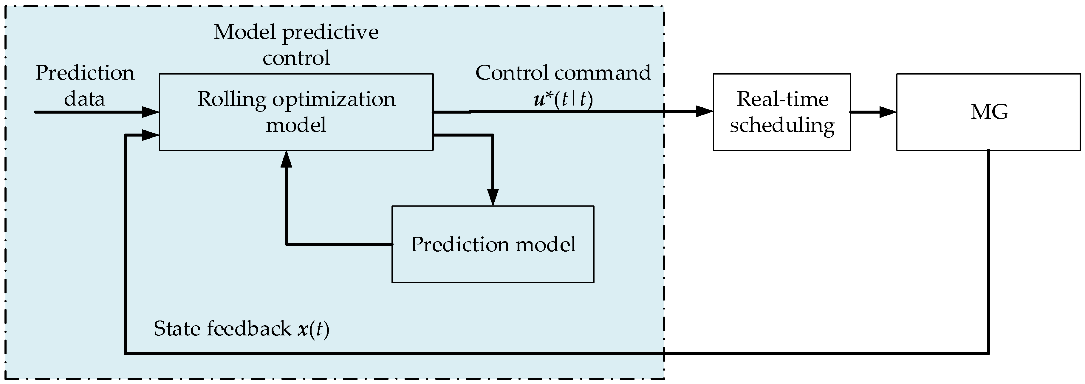
3.3.1. Model Predictive Control Framework

Rolling scheduling in fact is an online rolling optimization problem over a short period time, the whole scheduling time is divided into several scheduling periods and an optimal scheduling strategy is solved online in each scheduling period Three characteristics of predictive control makes it suitable for rolling scheduling:

(1)

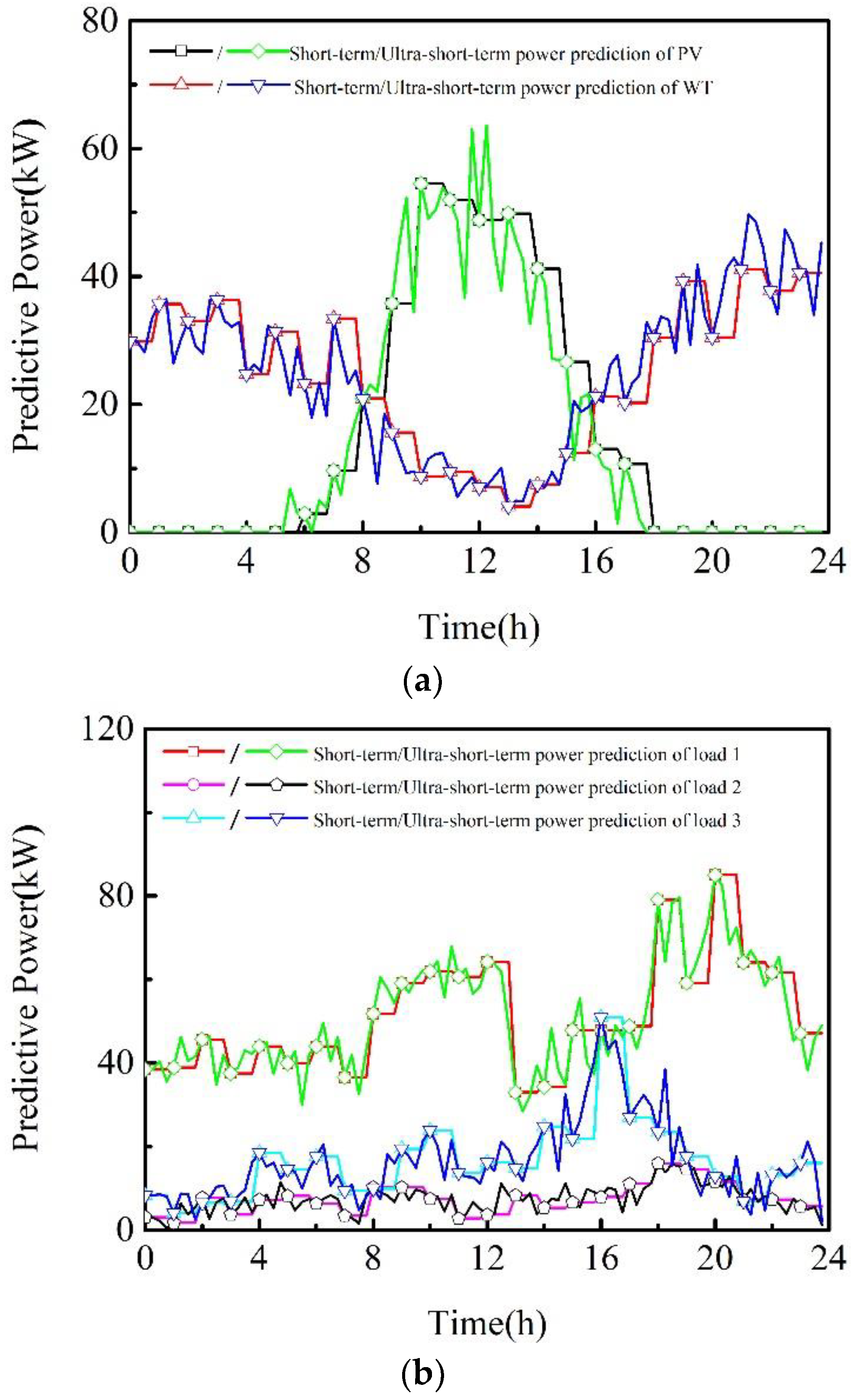
Prediction model: Based on the measured output data of generators and the predictive data of RES and load data in the next time period, this model is used to predict the future output of generators.

(2)

Rolling optimization: Repeated online optimization negates the influence caused by uncertain factors such as RE fluctuations.

(3)

Feedback control: The measured data feedback is used to correct the actual output state of the generators in the model and ensure that the next optimization calculation is based on the latest measured data.

Figure 3 is the framework of MPC (model predictive control, MPC) based rolling scheduling optimization framework. Use the measured state feedback and prediction data to solve an optimal control sequence. For example, the following equation is the optimal control sequence:

$${\mathit{U}}^{*}=[{\mathit{u}}^{*}(t|t),{\mathit{u}}^{*}(t+1|t),\cdots ,{\mathit{u}}^{*}(t+k-1|t)]$$

(18)

where $k$ is the prediction horizon. ${\mathit{U}}^{*}$ is the optimal control sequence for the following $k$ time periods solved at time. ${\mathit{u}}^{*}(t|t)$ is the optimal control rule for the first time period solved at time $t$, comprised of a vector of control variables. In this paper, the rolling time window length, that is, the prediction horizon, is $k=4\mathrm{h}$, time interval is $\Delta t=15\min$.

3.3.2. Decision Variables

Decision variables in this model is almost the same as that of the day-ahead optimization model with a slight difference of variable dimensions.

3.3.3. Objective Function and Constraints

In the traditional intraday rolling scheduling optimization mode for grid-connected MG, the mode only corrects the scheduling for DGs but not the unit commitment and load switching. Besides, for MG with high RE penetration, the randomness and the intermittent of sources and load have negative effect on stable operation of MG. Thus, in this intraday rolling scheduling optimization model, optimization for unit commitment and load switching is required. Also, the SOC of ETESS is expected to follow the day-ahead scheduling as possible. So, the objective function also consists of operation cost term F and decision regularization term C. F is basically the same as that in the day-ahead optimization model while C includes SOC deviation correction penalty of ETESS, PV and WT curtailment penalty, load switching scheduling correction penalty and unit commitment correction penalty of diesel generators. The objective function is described as follows:

$$\begin{array}{cc}\hfill y(\mathit{P},\mathit{u})& =F_{\mathrm{load}}({\mathit{u}}_{\mathrm{load}})-F_{\mathrm{ba}}({\mathit{P}}_{\mathrm{ba}},{\mathit{u}}_{\mathrm{ba}})-F_{\mathrm{de}}({\mathit{P}}_{\mathrm{de}},{\mathit{u}}_{\mathrm{de}})-F_{\mathrm{re}}({\mathit{P}}_{\mathrm{pv}},{\mathit{P}}_{\mathrm{wt}})\hfill \\ & +C_{\mathrm{dep}}({\mathit{P}}_{\mathrm{pv}},{\mathit{P}}_{\mathrm{wt}})+C_{\mathrm{crt}\text{\_}\mathrm{soc}}({\mathit{P}}_{\mathrm{ba}},{\mathit{u}}_{\mathrm{ba}})+C_{\mathrm{crt}\text{\_}\mathrm{ld}}({\mathit{u}}_{\mathrm{load}})+C_{\mathrm{crt}\text{\_}\mathrm{de}}({\mathit{u}}_{\mathrm{de}})\hfill \end{array}$$

(19)

where $C_{\mathrm{crt}\text{\_}\mathrm{soc}}({\mathit{P}}_{\mathrm{ba}},{\mathit{u}}_{\mathrm{ba}})$, $C_{\mathrm{crt}\text{\_}\mathrm{ld}}({\mathit{u}}_{\mathrm{load}})$, $C_{\mathrm{crt}\text{\_}\mathrm{de}}({\mathit{u}}_{\mathrm{de}})$ are the SOC error correction regularization term, load switching schedule correction regularization term and unit commitment correction regularization term. The meanings of other variables are already described in the day-ahead optimization objective function. This model executes every 15 min, obtaining the schedule results for the following 4 h and take the first 15 min result as the MPC decision command. The newly added regularization terms equations are described as follows:

$$C_{\mathrm{crt}\text{\_}\mathrm{soc}}={\beta }_{\mathrm{crt}\text{\_}\mathrm{soc}}{\displaystyle \sum _{t=1}^{T_2}({\displaystyle \sum _{j=1}^{n_{\mathrm{ba}}}[So{c}_{\mathrm{ba},j}(t)-So{c}_{\mathrm{ba},j}^{\mathrm{Day}\text{\_}\mathrm{ahead}}(t)]})}$$

(20)

$$C_{\mathrm{crt}\text{\_}\mathrm{ld}}={\beta }_{\mathrm{crt}\text{\_}\mathrm{ld}}{\displaystyle \sum _{t=1}^{T_2}({\displaystyle \sum _{k=1}^{n_{\mathrm{sdload}}}\begin{array}{l}\mathrm{abs}(u_{\mathrm{sdload},k}(t)-u_{\mathrm{sdload},k}^{\mathrm{Day}\text{\_}\mathrm{ahead}}(t))+\\ {\displaystyle \sum _{p=1}^{n_{\mathrm{ctload}}}\mathrm{abs}(u_{\mathrm{ctload},p}(t)-u_{\mathrm{ctload},p}^{\mathrm{Day}\text{\_}\mathrm{ahead}}(t))}\end{array}})}$$

(21)

$$C_{\mathrm{crt}\text{\_}\mathrm{de}}={\beta }_{\mathrm{crt}\text{\_}\mathrm{de}}{\displaystyle \sum _{t=1}^{T_2}({\displaystyle \sum _{i=1}^{n_{\mathrm{de}}}abs(u_{\mathrm{de},i}(t)-u_{\mathrm{de},i}^{\mathrm{Day}\text{\_}\mathrm{ahead}}(t))})}$$

(22)

where ${\beta }_{\mathrm{crt}\text{\_}\mathrm{soc}}$, ${\beta }_{\mathrm{crt}\text{\_}\mathrm{ld}}$, ${\beta }_{\mathrm{crt}\text{\_}\mathrm{de}}$ are the coefficients of SOC error correction regularization, load switching schedule correction regularization and unit commitment correction regularization. T₂ is the rolling window length, which is usually set to 4 h.

3.4. Comprehensive Criteria Based Quasi-Real-Time Coordinated Control

Although the prediction accuracy of RES and load have improved greatly in intraday rolling optimization model, errors still exist. The intraday rolling optimization model in this paper is performed once every 15 min and at the interval between two execution times, the unbalanced power caused by the prediction error should not be completely borne by the diesel generator (when it is the main source). Meanwhile, in order to improve the ability of ETESS actual SOC to follow the rolling optimization results, quasi-real-time unbalanced power can be used to correct the charge/discharge power of ETESS under some conditions. Therefore, in order to satisfy the mentioned requirements and further deal with the prediction error, this paper adds a control process with smaller timescale.

To improve calculation speed and reduce decision making time, a quasi-real-time coordinated control criterion system is developed in this paper, including quasi-real-time unbalanced power, power command of ETESS in rolling optimization and quasi-real-time SOC of ETESS. Different quasi-real-time coordinated control strategies based on different criteria states, as shown in

Table 1. Quasi-real-time coordinated control criterion system.

Quasi-Real-Time Power Imbalance	Power of ETESS in Rolling Optimization	Quasi-Real-Time SOC of ETESS
① $P_{\mathrm{ubl}}^{\mathrm{m}}(t)>0$	③ $P_{\mathrm{ba}}^{\mathrm{h}}(t)>0$	⑤ $So{c}_{\mathrm{ba}}^{\mathrm{m}}(t)>So{c}_{\mathrm{ba}}^{\mathrm{h}}(t)$
② $P_{\mathrm{ubl}}^{\mathrm{m}}(t)<0$	④ $P_{\mathrm{ba}}^{\mathrm{h}}(t)\le 0$	⑥ $So{c}_{\mathrm{ba}}^{\mathrm{m}}(t)\le So{c}_{\mathrm{ba}}^{\mathrm{h}}(t)$

where $P_{\mathrm{ubl}}^{\mathrm{m}}(t)$ is the measured quasi-real-time power imbalance value. $P_{\mathrm{ba}}^h(t)$ is the command value of rolling optimization for ETESS power. $So{c}_{\mathrm{ba}}^{\mathrm{m}}(t)$ is the measured quasi-real-time SOC value of ETESS. $So{c}_{\mathrm{ba}}^{\mathrm{h}}(t)$ is the scheduled SOC value of ETESS given by rolling optimization.

.

The quasi-real-time unbalanced power determines the type of DGs that can be used to adjust the unbalanced power and the adjustment direction of the power increment. When the quasi-real-time unbalanced power is greater than zero, it indicates that there is a power shortage in MG system and diesel generators and ETESS is determined to participate in the adjustment of unbalanced power. Conversely, when the quasi-real-time unbalanced power is less than zero, it indicates that there is a power surplus in MG system, all types of DGs can take part the adjustment of unbalanced power.

The ETESS power command value determined from rolling optimization can provide criteria for the decision of ETESS quasi-real-time charge/discharge state which is expected to follow the command from rolling optimization. Besides, the quasi-real-time SOC measurement of ETESS can also provide criteria for the decision of ETESS quasi-real-time charge/discharge state. When the quasi-real-time SOC measurement of ETESS is greater than the SOC determined from rolling optimization, the decision of ETESS is expected to increase the discharge power or reduce the charge power, so that SOC of ETESS is close to the scheduled value as soon as possible. Likewise, when the measurement is less than the scheduled value, it is determined to reduce discharge power or increase charge power.

The 8 types of control strategies can be obtained by arranging and combining the above criteria, and the adjustment priorities of DGs in different types of control strategies may be different. When the quasi-real-time unbalanced power is less than zero, if the DER with highest priority cannot fully compensate the unbalanced power, PV or WT system will reduce output power until it is fully compensated.

(1)

When ①③⑤ are satisfied, increase the discharge power of ETESS with high priority. The increment $\Delta P_{\mathrm{ba}}^{\mathrm{m}}(t)$ is calculated by SOC error and rated capacity, as described by the following equation:

$$\Delta P_{\mathrm{ba}}^{\mathrm{m}}(t)=\min (P_{\mathrm{ba},\mathrm{n}}^{\mathrm{dis}}-P_{\mathrm{ba}}^{\mathrm{h}}(t),\frac{E_{\mathrm{ba},\mathrm{n}}(So{c}_{\mathrm{ba}}^{\mathrm{m}}(t)-So{c}_{\mathrm{ba}}^{\mathrm{h}}(t)){\eta }_{\mathrm{ba},\mathrm{dis}}}{\Delta T_{\mathrm{rest}}},P_{\mathrm{ubl}}^{\mathrm{m}}(t))$$

(23)

where $\Delta T_{\mathrm{rest}}(t)$ is the resting time until next rolling optimization.

(2)

When ①③⑥ are satisfied, increase the output of diesel generators with high priority. The increment $\Delta P_{\mathrm{de}}^{\mathrm{m}}(t)$ takes rated power and spinning reserve margin into consideration, as described by the following equation:

$$\Delta P_{\mathrm{de}}^{\mathrm{m}}(t)=\min (P_{\mathrm{de},\mathrm{n}}-R_{\mathrm{de}}(t)-P_{\mathrm{de}}^{\mathrm{h}}(t),P_{\mathrm{ubl}}^{\mathrm{m}}(t))$$

(24)

where $P_{\mathrm{de}}^{\mathrm{h}}(t)$ is the command of rolling optimization for diesel generators and $R_{\mathrm{de}}(t)$ is the spinning reserve margin.

(3)

When ①④⑤ are satisfied, decrease the charge power of ETESS with high priority. $\Delta P_{\mathrm{ba}}^{\mathrm{m}}(t)$ is described by the following equation:

$$\Delta P_{\mathrm{ba}}^{\mathrm{m}}(t)=\min (-P_{\mathrm{ba}}^{\mathrm{h}}(t),P_{\mathrm{ubl}}^{\mathrm{m}}(t))$$

(25)

(4)

When ①④⑥ are satisfied, the strategy is the same as Equation (2).

(5)

When ②③⑤ are satisfied, decrease the output of diesel generators with high priority. The increment $\Delta P_{\mathrm{de}}^{\mathrm{m}}(t)$ needs to take minimum load limitation into consideration, as described by the following equation:

$$\Delta P_{\mathrm{de}}^{\mathrm{m}}(t)=\max ({\beta }_{\mathrm{de},\min }{P}_{\mathrm{de},\mathrm{n}}-P_{\mathrm{de}}^{\mathrm{h}}(t),P_{\mathrm{ubl}}^{\mathrm{m}}(t))$$

(26)

(6)

When ②③⑥ are satisfied, decrease the discharge power of ETESS with high priority. $\Delta P_{\mathrm{ba}}^{\mathrm{m}}(t)$ is described by the following equation:

$$\Delta P_{\mathrm{ba}}^{\mathrm{m}}(t)=-\min (P_{\mathrm{ba}}^{\mathrm{h}}(t),P_{\mathrm{ubl}}^{\mathrm{m}}(t))$$

(27)

(7)

When ②④⑤ are satisfied, the strategy is the same as Equation (5).

(8)

When ②④⑥ are satisfied, increase the charge power of ETESS with high priority. $\Delta P_{\mathrm{ba}}^{\mathrm{m}}(t)$ is described by the following equation:

$$\Delta P_{\mathrm{ba}}^{\mathrm{m}}(t)=\max (P_{\mathrm{ba},\mathrm{n}}^{\mathrm{cha}}-P_{\mathrm{ba}}^{\mathrm{h}}(t),\frac{E_{\mathrm{ba},\mathrm{n}}(So{c}_{\mathrm{ba}}^{\mathrm{m}}(t)-So{c}_{\mathrm{ba}}^{\mathrm{h}}(t)){\eta }_{\mathrm{ba},\mathrm{cha}}}{\Delta T_{\mathrm{rest}}},P_{\mathrm{ubl}}^{\mathrm{m}}(t))$$

(28)

3.5. Real-Time Correction Control of Hybrid Energy Storage

Since the time scale of real-time correction control is short, DSGs with low response speed such as PV and WT are not incorporated into this process. Therefore, real-time correction process of MGCC only considers HESS remote adjustment. During the process of real-time coordinated control model, HESS is used to compensate second-level power imbalance. ETESS compensates the slowly varying component in power imbalance, while PTESS compensates the fast-varying component. Besides, to solve the SOC limit violation problem, a PTESS energy calibration method is developed to ensure the PTESS can maintain the ability to charge/discharge continuously.

This paper uses the first order low-pass filter (FOLPF) algorithm to calculate the component power for PTESS. The transfer function of FOLPF algorithm can be described as follows:

$$P_{\mathrm{nbl}}^{\mathrm{sf}}(s)=\frac{1}{1+s{T}_{\mathrm{stab}}}{P}_{\mathrm{nbl}}^{\mathrm{s}}(s)$$

(29)

where $P_{\mathrm{nbl}}^{\mathrm{s}}(s)$ $P_{\mathrm{nbl}}^{\mathrm{sf}}(s)$, are the power imbalance and the Laplace transform of its low-frequency component. $T_{\mathrm{stab}}$ is the time constant of low-pass filter; s is the Laplacian operator.

If s is substituted by d/dt and use $\Delta t$ as the calculation step, then the equation of FOLPF in time domain can be described as follows:

$$P_{\mathrm{nbl}}^{\mathrm{sf}}(t)=\frac{T_{\mathrm{stab}}}{\Delta t+T_{\mathrm{stab}}}{P}_{\mathrm{nbl}}^{\mathrm{sf}}(t-\Delta t)+\frac{\Delta t}{\Delta t+T_{\mathrm{stab}}}{P}_{\mathrm{nbl}}^{\mathrm{s}}(t)$$

(30)

where $P_{\mathrm{nbl}}^{\mathrm{sf}}(t)$, $P_{\mathrm{nbl}}^{\mathrm{sf}}(t-\Delta t)$ are the low-frequency component of power imbalance at the current time period and the last time period; $P_{\mathrm{nbl}}^{\mathrm{s}}(t)$ is the power imbalance at the current time period; $\Delta t$ is the data sampling interval, which is the timescale of real-time coordinated control, $\Delta t=5\mathrm{s}$.

ETESS is responsible for dealing with the lower frequency component $\Delta P_{\mathrm{ba}}^{\mathrm{s}}(t)$, while the high-frequency component is dealt with by PTESS. The real-time coordinated control command for ETESS and PTESS are:

$$P_{\mathrm{ba}}^{\mathrm{s}}(t)=P_{\mathrm{ba}}^{\mathrm{s}}(t-\Delta t)+\Delta P_{\mathrm{ba}}^{\mathrm{s}}(t)=P_{\mathrm{ba}}^{\mathrm{s}}(t-\Delta t)+P_{\mathrm{nbl}}^{\mathrm{sf}}(t)$$

(31)

$$P_{\mathrm{sc}}^{\mathrm{s}}(t)=P_{\mathrm{nbl}}^{\mathrm{s}}(t)-P_{\mathrm{ba}}^{\mathrm{s}}(t)$$

(32)

Considering the ETESS is expected to follow intraday rolling optimization schedule, the time constant of FOLPF should be able to adjust adaptively so that the ETESS can compensate the low-frequency component of power imbalance and make its SOC close to the rolling optimization result at the same time. To achieve this, a rule for adjusting the time constant in FOLPF is developed:

$$T_{\mathrm{stab}}(t)=[1-\lambda (t)\cdot (So{c}_{\mathrm{ba}}^{\mathrm{s}}(t)-So{c}_{\mathrm{ba}}^{\mathrm{h}}(t))]T_{\mathrm{stab}}^{\mathrm{ref}}$$

(33)

$$\lambda (t)=\mathrm{sign}(P_{\mathrm{nbl}}^{\mathrm{s}}(t))\cdot {\lambda }_{\mathrm{T}}^{\mathrm{ref}}$$

(34)

where $T_{\mathrm{stab}}^{\mathrm{ref}}$ is the reference for time constant; $So{c}_{\mathrm{ba}}^{\mathrm{s}}(t)$ is the SOC of ETESS measured in real-time; $\lambda (t)$ is the adjusting coefficient; ${\lambda }_{\mathrm{T}}^{\mathrm{ref}}$ is the reference for the adjusting coefficient; $\mathrm{sign}(\cdot )$ is the sign function, whose value is 1 if the variable is positive, −1 if negative and 0 if the variable is 0.

When power imbalance $P_{\mathrm{nbl}}^{\mathrm{s}}(t)$ is greater than 0, $\lambda (t)$ is a positive value. If ETESS SOC is also greater than the rolling optimization value, then $T_{\mathrm{stab}}(t)\text{<}{T}_{\mathrm{stab}}(t)$ and the power adjustment $\Delta P_{\mathrm{ba}}^{\mathrm{s}}(t)$ dispatched to ETESS will increase, causing the SOC to decrease rapidly to the optimal value. But if the SOC is less than the rolling optimization value, then $\Delta P_{\mathrm{ba}}^{\mathrm{s}}(t)$ will decrease, slowing down the offset velocity of SOC. Same effects are expected when $P_{\mathrm{nbl}}^{\mathrm{s}}(t)$ is less than 0.

But when the SOC of PTESS is too high or too low, positive and negative high-frequency power imbalance cannot be compensated at the same time, requiring blocking PTESS’s charging function or discharging function. If the SOC of PTESS is too low, the discharging function is blocked and PTESS only compensates the negative high-frequency power imbalance, while the positive high-frequency component is compensated by diesel generators. If the SOC of PTESS is too high, the charging function is blocked and PTESS only compensates the positive high-frequency power imbalance, while the negative high-frequency component is compensated by diesel generators. When the PTESS’s SOC is back around the middle value, the charge/discharge function is unblocked.

4. Case Study

This paper uses the topology shown in Figure 1 as the study case. This MG contains two diesel generators with rated power 50 kW, a wind power system with rated power 60 kW, a PV system with rated power 70 kW, a HESS consists of lead acids batteries (50 kW/200 kWh) and SC (50 kW/5 kWh) and three loads (load 1 is an important load, 2 and 3 are secondary loads). Simulation software Matlab R2014a is used and ILOG CPLEX solver is used in day-ahead and intraday model. Our code is available upon request.

4.1. Basic Data

The basic data analyzed in this example includes the parameters of each power generation unit in the MG, multi-time scale coordinated control related parameters, the short-term power prediction results, ultra-short-term power prediction and real-time power data of WT systems, PV systems and loads. The parameters of DSGs, RES, HESS, and multi-timescale coordinated control models are as shown in

Table 2. Parameters of diesel generator.

Serial Number of DSG	Rated Power (kW)	Startup Cost (CNY/Per Time)	Shutdown Cost (CNY/Per Time)	Coefficient of Operation Cost (CNY/kWh)	Fuel Cost (CNY/kWh)	Fuel Curve Slope (L/kWh)	Minimum Load Factor (%)
1	50	2	2	0.0088	7	0.	30
2	50	2	2	0.0088	7	0.3	30

,

Table 3. Parameters of renewable energy sources.

Type	Rated Power (kW)	Coefficient of Operation Cost (CNY/kWh)
Wind power	50	0.0296
PV power	50	0.0096

,

Table 4. Parameters of HESS.

Type	Rated Power/Capacity (kW/kWh)	Initial Investment Cost (CNY/kWh)	Coefficient of Operation Cost (CNY/kWh)	Energy Per Unit Capacity (kWh)	Permitted SOC Range (%)	SOC Warning Range (%)	Initial SOC (%)
ETESS	50/200	2	0.0088	250	[10, 90]	[30, 70]	50
PTESS	50/5	11.4	0	∞	[10, 90]	[30, 70]	50

,

Table 5. Parameters of multi-timescale coordinated control (day-ahead and intraday model).

Energy Balance Error in a Cycle (%)	DSG Minimum Operation (Shutdown) Time (h)	Reserve Capacity (kW)	Regularization Parameter of RE Curtailment	Regularization Parameter of Power Shortage	Regularization Parameter of DSG Unit Commitment Correction	Regularization Parameter of SOC Error Correction
10	2	10	5000	10000	10000	500

and

Table 6. Parameters of multi-timescale coordinated control (Quasi-real-time and real-time model).

Adjusting Coefficient for Time Constant of FOLPF	Reference Value for Time Constant of FOLPF
15	30

.

Short-term and ultra-short-term power prediction results are shown in Figure 4:

4.2. Analysis of Multi-Timescale Coordinated Control

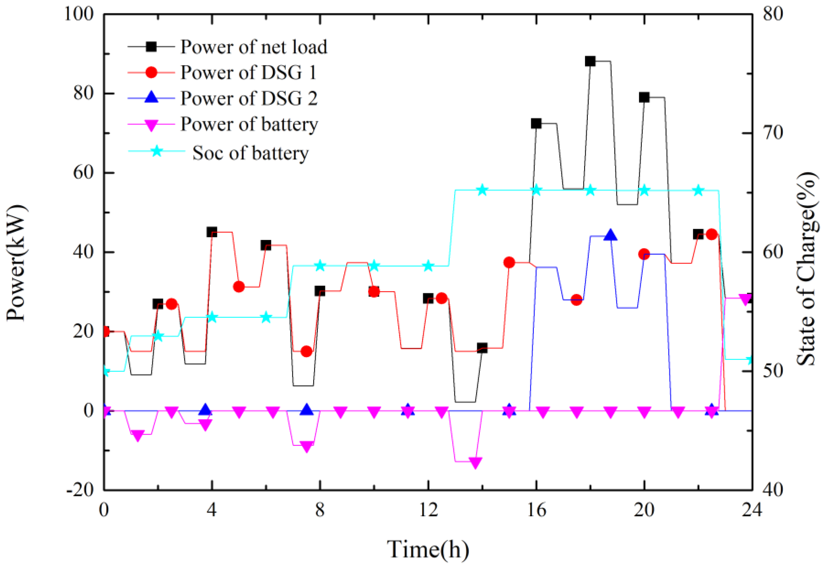
4.2.1. Analysis of Day-Ahead Optimization

The day-ahead scheduling results are shown in Figure 5. The startup and shutdown schedule of two DSGs are: DSG1 runs during 0:00–23:00 and DSG2 runs during 16:00–21:00. Because during 16:00–21:00, the predicted load is increasing and the predicted RES power is decreasing (due to the fading of sunlight), DSG2 is activated to generate power for the load within the MG. During 0:00–23:00, at least one DSG is running as the main power supply for the net load. When the net load is less than the minimum load factor of DSG, ETESS starts to charge to ensure DSG operates normally. After 21:00, the predicted net load starts to decrease and ETESS needs to discharge to make its SOC value back to around 0.5, so DSG2 needs to be shut down during 21:00–24:00 and as for DSG1, 23:00–24:00. Therefore, ETESS is the main power supply for the MG after 23:00 and its SOC value drop backs to around 0.5.

In the day-ahead optimization results, there is no need to shed load and limit the power of RES, so the corresponding regularization term is 0. To verify the effects of RES curtailment and power shortage regularization term, a comparison test is setup. In the comparison test, RES curtailment and power shortage regularization term are neglected and the other conditions are kept the same. The day-ahead optimization results of the comparison test are shown in

Table 7. Comparison test for the verification of effects of regularization terms in day-ahead optimization model.

Day-Ahead Optimization Results	Without Regularization Terms	With Regularization Term
RE curtailment (%)	0.00095619	0
Power shortage (%)	28.3567	0
MG operation cost (CNY)	−1049.9027	−645.8309

. As the results suggest, without regularization terms in the day-ahead optimization model, the power shortage percentage can reach as high as 28.3567% and the system operation cost is 62.57% less than the cost when regularization is taken into account. These results show that generation cost of standalone MG is still high. Even when the electricity selling price is 1.5 CNY, the marginal generation cost is still higher than marginal usage cost. Therefore, for stand-alone MG that needs to ensure the reliability of power supply, it is necessary to sacrifice some economic benefits to reduce the load power shortage. An effective way is to add power shortage regularization term in day-ahead optimization model.

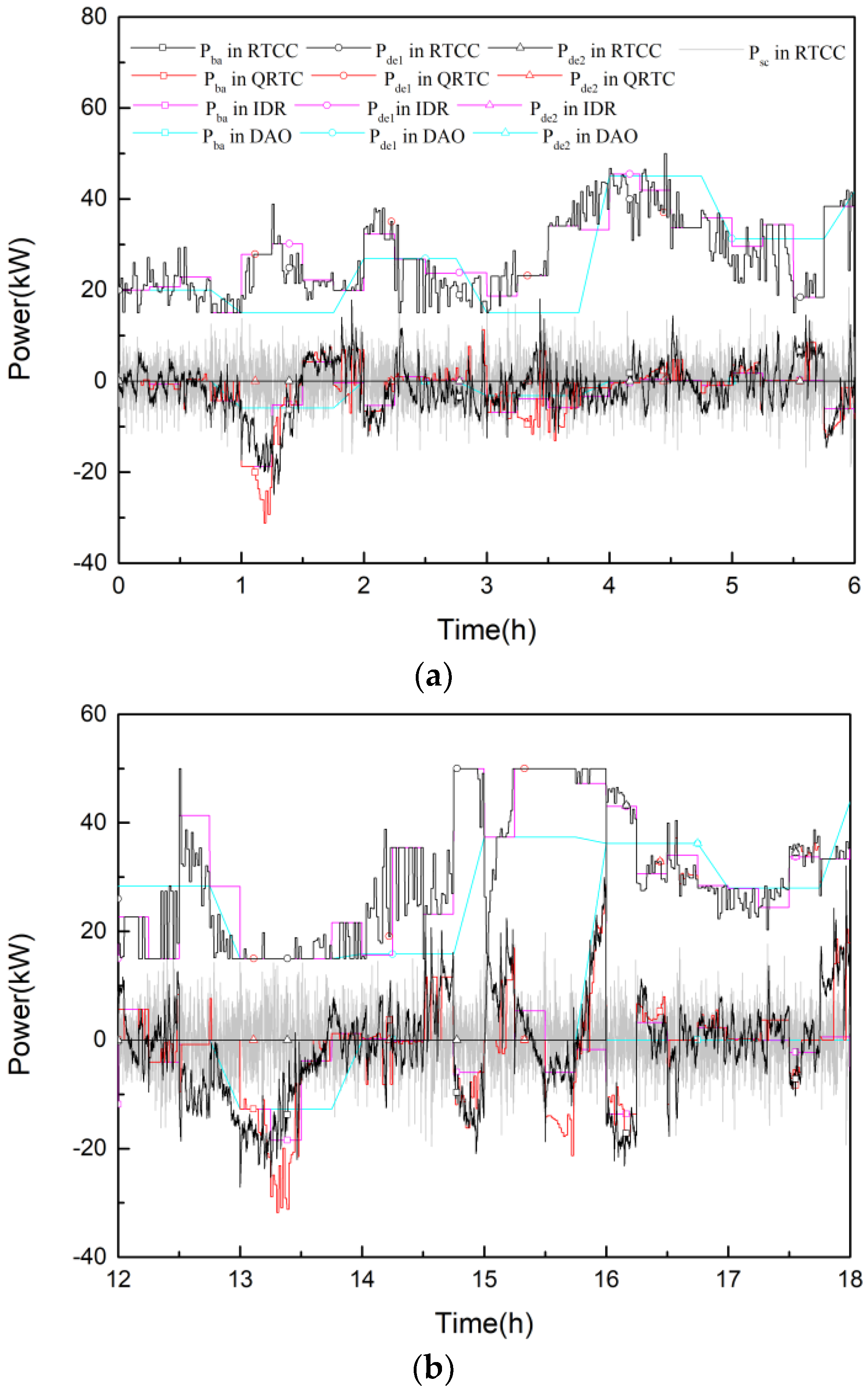
4.2.2. Analysis of Intraday, Quasi-Real-Time and Real-Time Coordinated Control

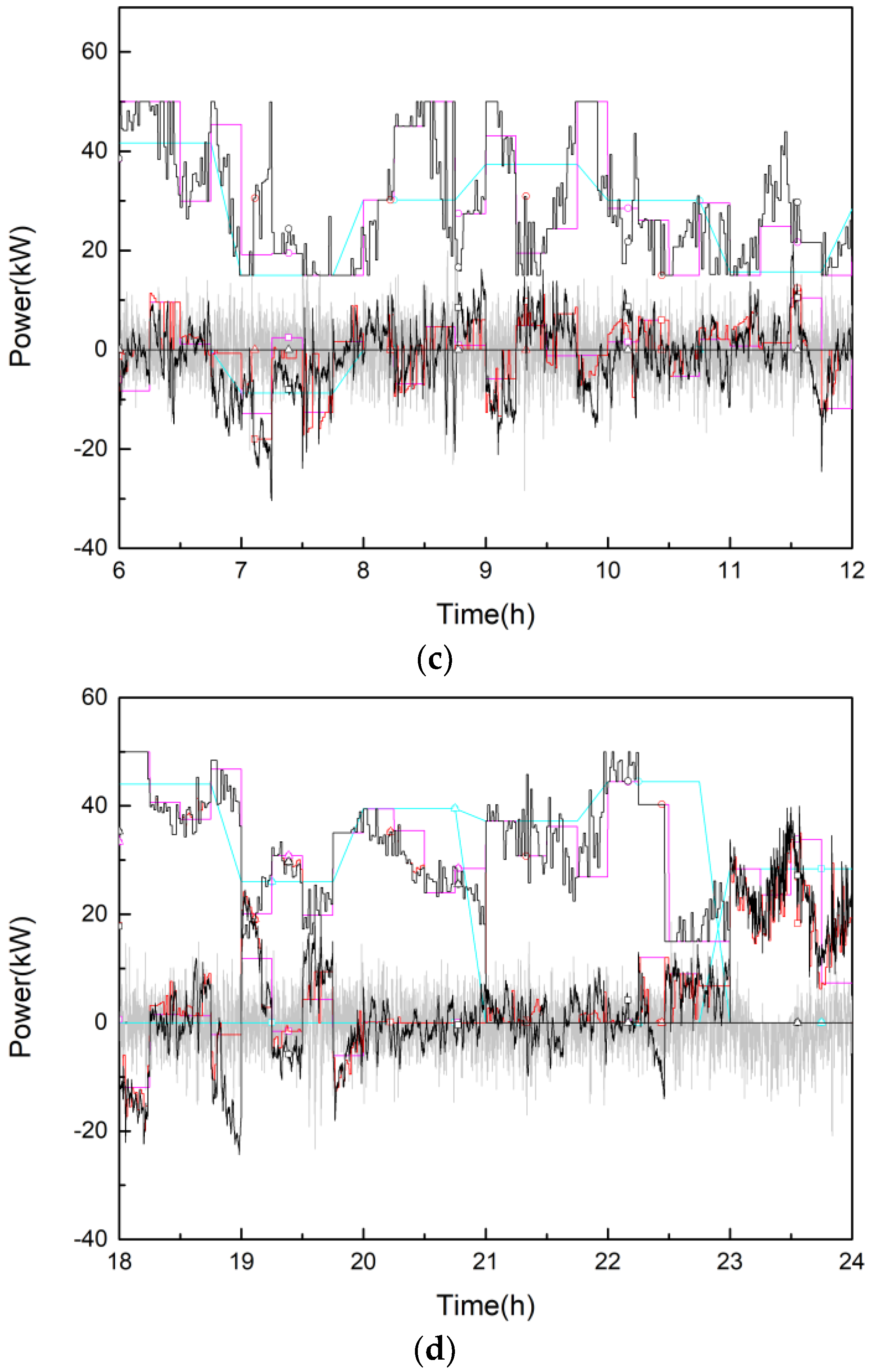
Since intraday rolling optimization, quasi-real-time and real-time coordinated control all need to use measured data as the input of the control algorithm, the coordinated control strategy decisions of these three timescales are strongly coupled. that is, the control result of shorter timescale will affect the decision of longer timescale. Therefore, the case analysis of these three parts are discussed together in this section. Figure 6 shows the results (0–24 h) of multi-timescale coordinated control case study.

As Figure 6 shows, the short-term and ultra-short-term forecasts have small errors, so there is no need to correct the startup and shutdown plan of DSGs in intraday rolling optimization. Under the condition that the plan follows the day-ahead scheduling result, observe the changing pattern of the operating power of DSG in various timescales:

(1)

The essential of seconds-scale real-time coordinated control is to use HESS to compensate the power imbalance in the interval of quasi-real-time coordinated control, so the power curve of DSG in real-time coordinated control is basically overlapped with that in quasi-real-time coordinated control.

(2)

The power curve of DSG is more accurate in the shorter timescale. Compared to real-time power curve, the mean error of quasi-real-time curve is 0.19% while the mean error of intraday rolling curve is 11.73% and for day-ahead scheduling, 26.09%.

Since the charging and discharging time of the PTESS is short, usually in the scale of seconds, the HESS only controls the ETESS in the day-ahead, intraday, quasi-real-time timescale, while the PTESS is only coordinated in real-time timescale to suppress the high frequency unbalanced power. Observe the changing characteristics of the operating power of ETESS in various timescales:

(1)

ETESS needs to compensate the low frequency unbalanced power in real-time timescale, so its real-time operating power curve is slightly different from the quasi-real-time curve.

(2)

Though intraday and day-ahead curves differ from the real-time curve greatly, they still reflect the overall change of the energy of ETESS.

Figure 7 shows the SOC curve of ETESS in various timescales and suggests that the real-time SOC curve can follow the day-ahead schedule accurately. This is due to introducing SOC error correction regularization term in intraday rolling model, comprehensive criteria in quasi-real-time model and adaptively adjusted time constant of FOLPF in real-time model. It can be seen from this figure that PTESS charge and discharge frequently to compensate the high frequency unbalanced power. If ETESS is used instead, the frequent charge and discharge activity will greatly reduce its cycle lifetime. During 23:00−24:00, DSGs are shut down and ETESS becomes the main power supply and its SOC is higher than the day-ahead schedule, so the system needs to compensate positive unbalanced power. The time constant of FOLPF decreases and the duty to compensate positive high frequency power imbalance shifts from PTESS to ETESS, making the SOC of ETESS falls to the scheduled value and the SOC if PTESS rises up quickly.

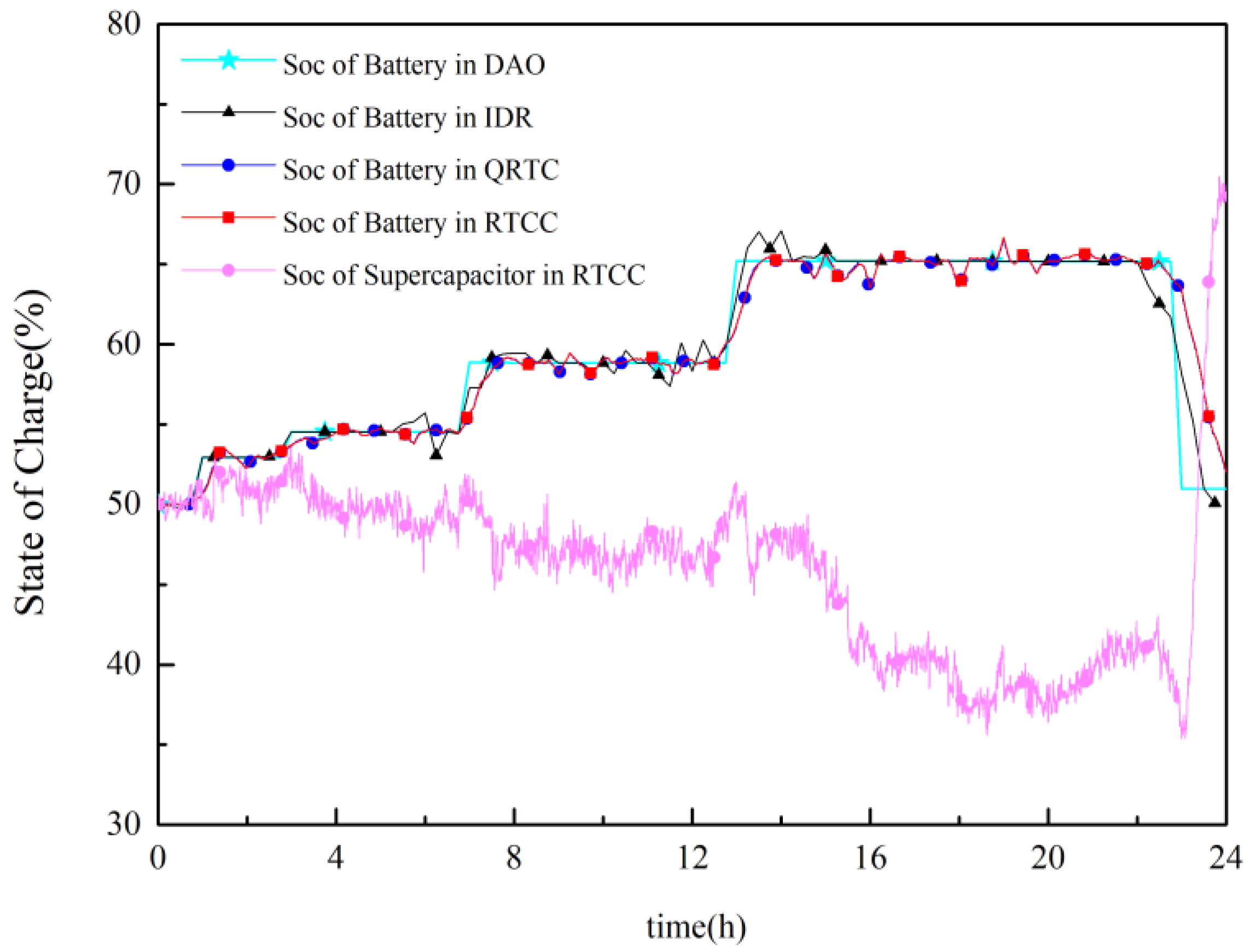
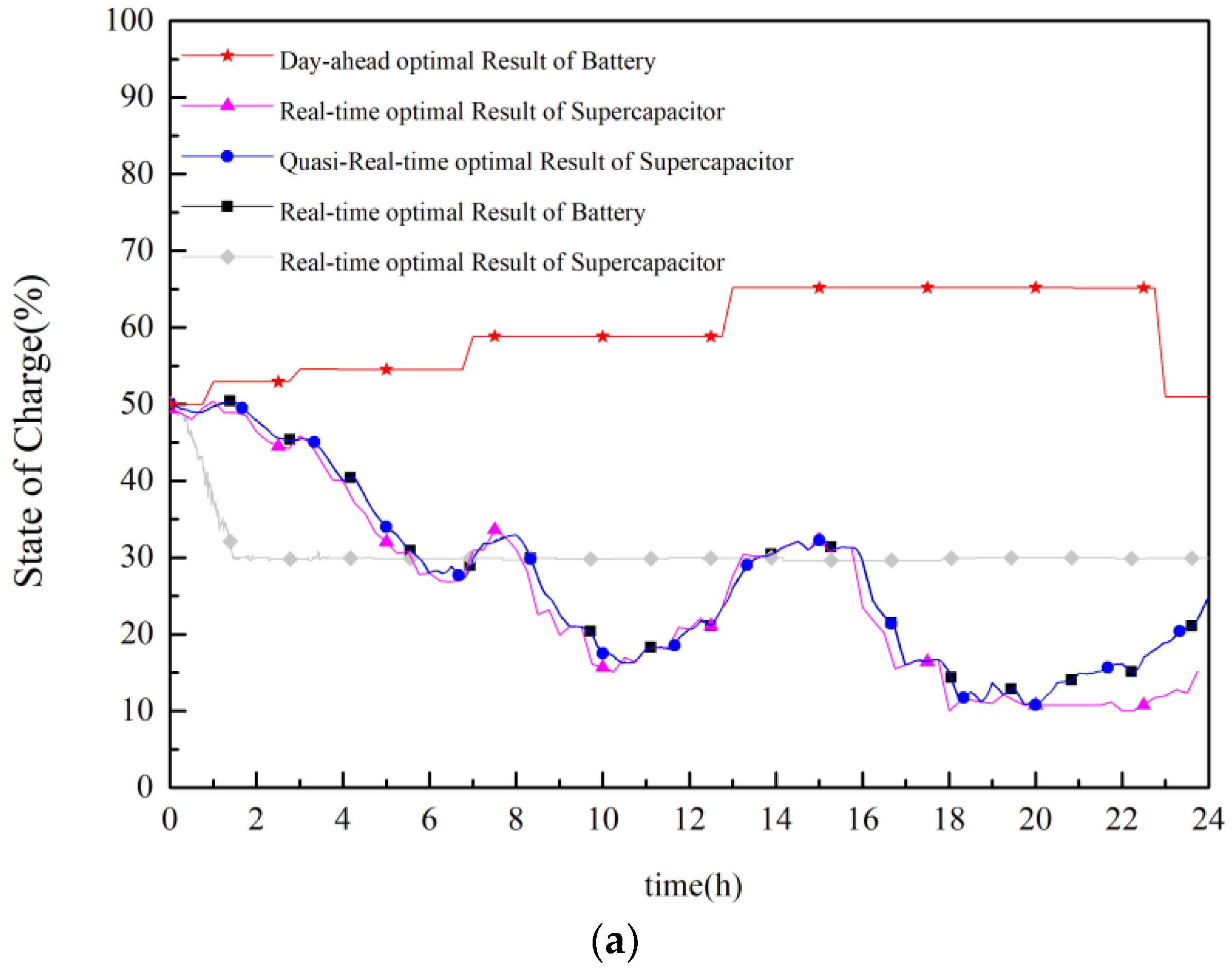
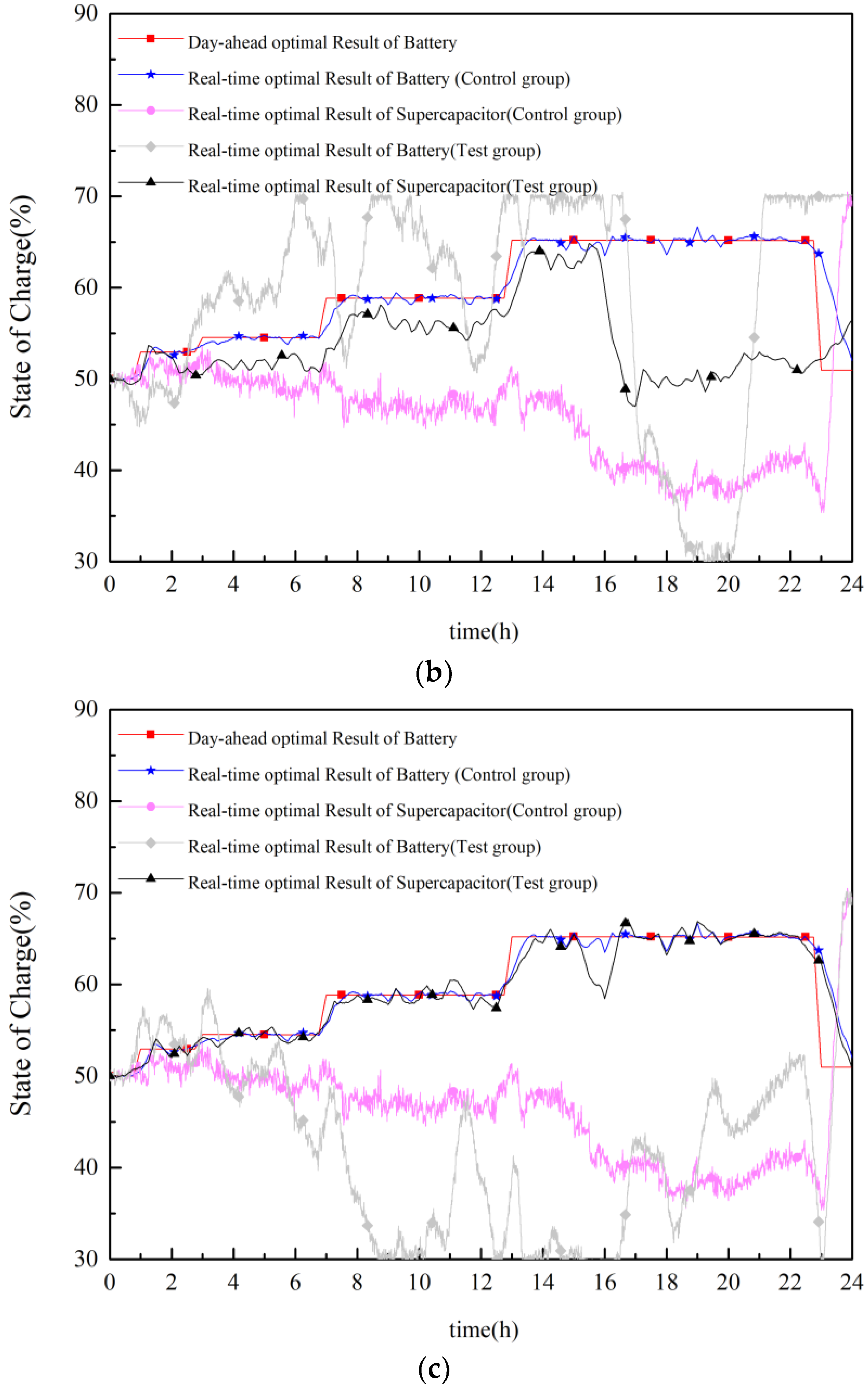
4.2.3. Analysis of Daily SOC Balance of ETESS

The SOC of ETESS being balanced at the beginning and end of the daily cycle is one the factors that MG can operate stably. To achieve this goal, this paper makes some improvements in four aspects: introduce daily SOC balance constraint of ETESS in day-ahead scheduling. Add an SOC error regularization term in the objective function of intraday rolling optimization. Use comprehensive criteria to decide the priority of dispatching each DG in quasi-real-time coordinated control, further reducing the SOC error. Use adaptively adjusted time constant in FOLPF to adjust the SOC of ETESS. To analyze the effects of the above methods on daily SOC balance, a comparison test is conducted and the results are shown in Figure 8:

Figure 8a shows the SOC waveforms when ETESS SOC error regularization is ignored in intraday rolling optimization. In this case, the ETESS SOC does not follow the day-ahead schedule and the value even drops below 30% in period 24:00. Meanwhile, because the ETESS SOC stays lower than the day-ahead schedule, when the seconds-timescale power imbalance is negative, time constant in FOLPF decrease adaptively, dispatching more negative unbalanced power to ETESS and less to PTESS, making PTESS SOC stays at a very low level.

Figure 8b shows the SOC waveforms when directly prioritize the adjustment of ETESS instead of considering comprehensive criteria in quasi-real-time coordinated control. The figure suggests the ETESS SOC error at the beginning and end of the day period is small but the SOC curve fails to follow the day-ahead schedule. This is because both positive and negative unbalanced power are compensated by ETESS. Since the ETESS SOC will deviate from the day-ahead schedule when power imbalance is very great. Besides, adjustment of time constant of FOLPF is only applicable in SOC fine-tuning but not large deviation.

Figure 8c shows the SOC waveforms when directly prioritize the adjustment of DSGs instead of considering comprehensive criteria in quasi-real-time coordinated control. The real-time ETESS SOC can follow the day-ahead schedule but due to the lack of adjustment of ETESS SOC in quasi-real-time coordinated control, the ETESS SOC regulation pressure is larger in real-time coordinated control, increasing the risk of PTESS’s energy exceeding the limit.

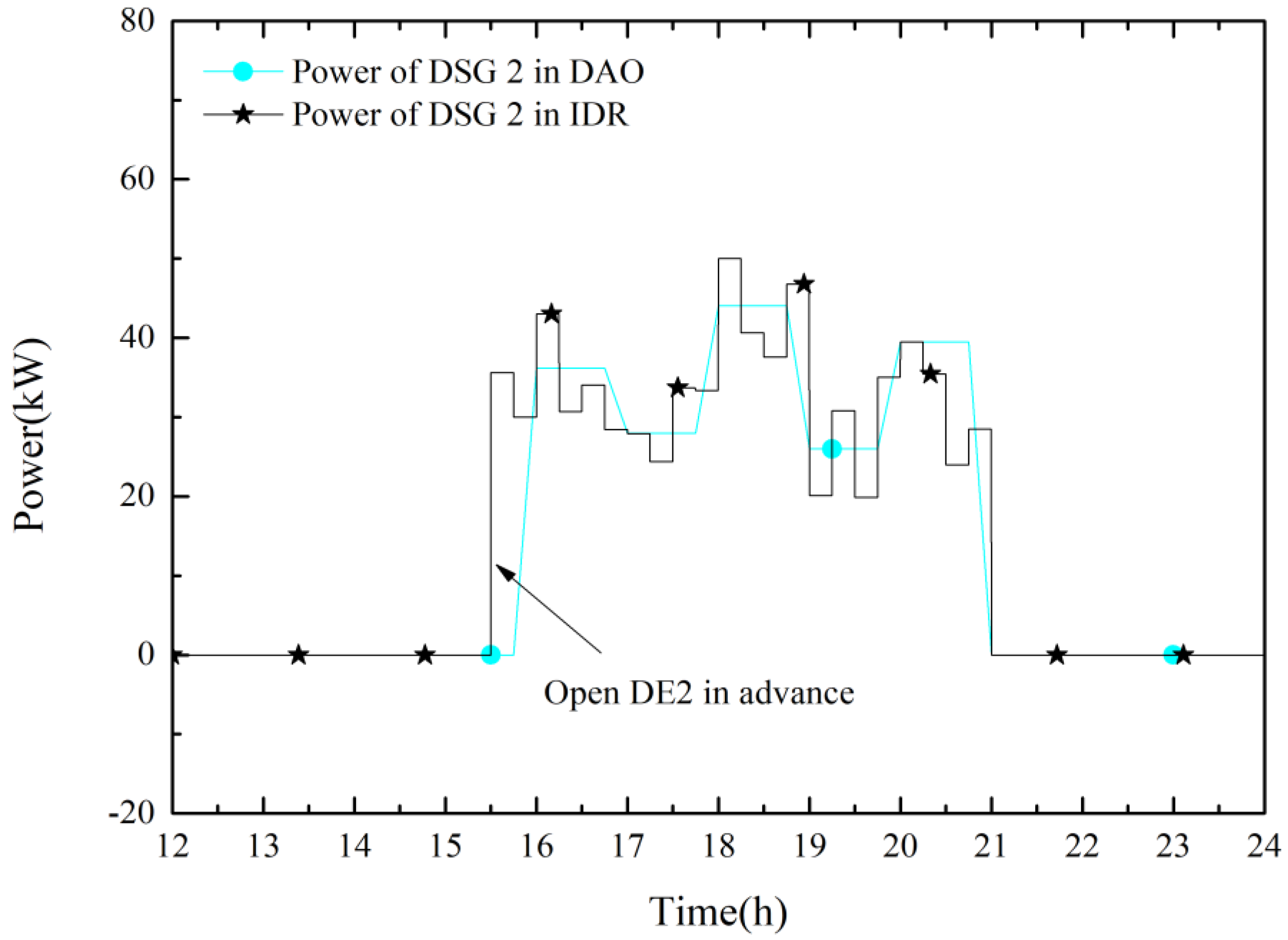
4.2.4. Analysis of the DSG Unit Commitment Correction Regularization

To verify the effects of the DSG unit commitment correcting regularization, this study modifies the day-ahead load prediction data to increase its prediction error, making the prediction data during 15:30–16:00 far less than the actual predicted data and the real-time data. The day-ahead and intraday unit commitment are shown in Figure 9.

Figure 9 shows when the prediction errors are so large that the system stability is threatened, the soft constraint which requires the unit commitment to follow the day-ahead schedule in intraday rolling optimization model, will lose its effect. The problem can be addressed by bringing the day-ahead schedule 0.5 h forward.

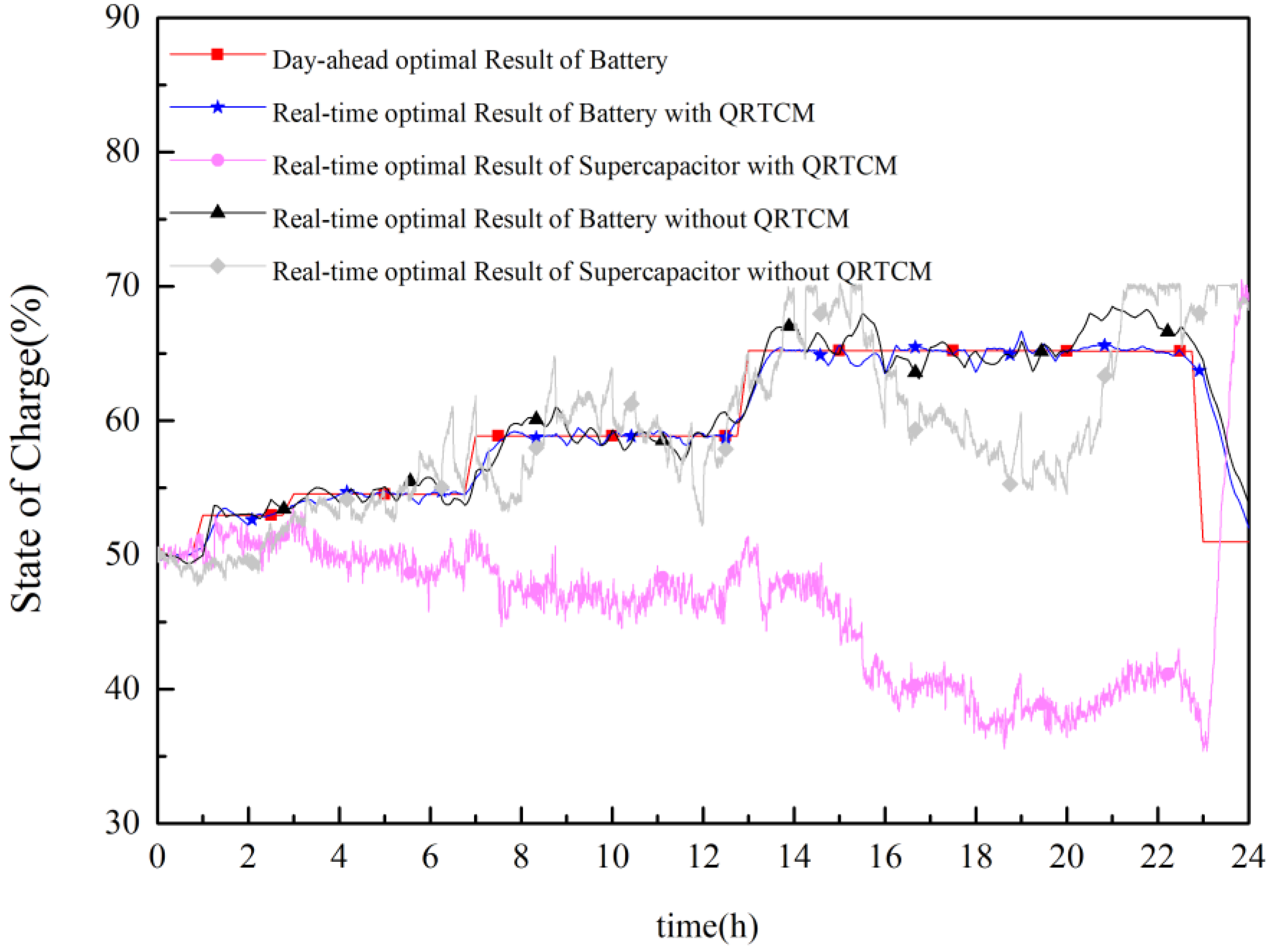
4.2.5. Analysis of the Necessity of Introducing Quasi-Real-Time Coordinated Control

The quasi-real-time coordinated control strategy is based on fixed logic rules and executes every minute. Introducing this model is to provide a transitional 1-min-timescale control between 15-min-timescale and 5-s-timescale control, smoothing the fluctuation by adjusting the power command of source and energy storage. Besides, the quasi-real-time coordinated control model uses comprehensive criteria to prioritize the dispatch of DGs, ensuring the ETESS SOC can follow the day-ahead schedule as possible. To verify this effect, a comparison test is set up, ignoring the quasi-real-time model while other conditions are kept the same. The test results are shown in Figure 10.

It can be seen from Figure 10 that ETESS SOC can follow the day-ahead schedule but has larger fluctuation when quasi-real-time model is ignored. In a MG that has small ETESS capacity, the risk of energy exceeding limit is greater. Besides, the PTESS SOC exceeds the limit multiple times because without the 1-min-timescale power imbalance compensation process, HESS needs to compensate unbalanced power every 5 s in a 15 min period. With such great regulating pressure, comes with the great risk of PTESS SOC exceeding the limit. In other words, introducing quasi-real-time coordinated control can enable ETESS SOC to follow the day-ahead schedule more accurately and reduce the operation risk of HESS.

5. Conclusions

This paper proposes a multi-timescale coordinated control scheme for stand-alone MG, consisting of “day-ahead optimization + intraday rolling + quasi-real-time correction + real-time coordinated control.” The day-ahead model uses economic benefit as objective to schedule unit commitment and load switching. In the intraday rolling model, three regularization terms are introduced as soft constraint, which are the SOC error correction regularization term, load switching schedule correction regularization term and unit commitment correction regularization term. In the quasi-real-time model, comprehensive criteria are used to prioritize the adjustment of every DG. In the real-time model, an improved FOLPF algorithm is used to decide the power command for HESS.

From the case study analysis, the following conclusions can be drawn:

(1)

Introduce power shortage regularization term in day-ahead optimization model can significantly improve the power supply reliability but at the cost of some economic profit.

(2)

Based on ultra-short-term forecasting, which has smaller prediction error, the intraday rolling optimization model can adjust the day-ahead schedule for DGs output power appropriately. When the day-ahead prediction error is large, DG unit commitment and load switching schedule will be correct to the robustness of the MG system.

(3)

To keep the ETESS SOC balance at the beginning and end of the day period, it is necessary to add ETESS SOC error regularization term in the intraday rolling optimization model. Besides, the comprehensive criterial proposed in quasi-real-time model can improve the ETESS’s ability to follow the day-ahead schedule and reducing the HESS operations risk at the same time.

In the future, further research can be conducted in these aspects:

(1)

To overcome the shortcomings of large error in day-ahead power prediction and increase the credibility of the optimization results, uncertainty optimization theory can be introduced, such as robust optimization, fuzzy programming and stochastic programming.

(2)

In large scale stand-alone MG system, it may contain multiple HESSs. How to manage the charge and discharge commands and the SOC of each HESS in quasi-real-time and real-time timescale, is a problem to be solved.

References

1. Hartono, B.S.; Budiyanto; Setiabudy, R. Review of microgrid technology. In Proceedings of the 2013 International Conference on QiR, Yogyakarta, Indonesia, 25–28 June 2013. [Google Scholar]
2. Lasseter, R.H.; Paigi, P. Microgrid: A conceptual solution. In Proceedings of the 2004 IEEE 35th Annual Power Electronics Specialists Conference, Aachen, Germany, 20–25 June 2004. [Google Scholar]
3. He, M.; Giesselmann, M. Reliability-constrained self-organization and energy management towards a resilient microgrid cluster. In Proceedings of the 2015 IEEE Power & Energy Society Innovative Smart Grid Technologies Conference (ISGT), Washington, DC, USA, 18–20 February 2015. [Google Scholar]
4. Hatziargyriou, N.; Asano, H.; Iravani, R.; Marnay, C. Microgrids. IEEE Power Energy Mag. 2007, 5, 78–94. [Google Scholar] [CrossRef]
5. Dougal, R.A.; Liu, S.; White, R.E. Power and life extension of battery-ultracapacitor hybrids. IEEE Trans. Compon. Packag. Technol. 2002, 25, 120–131. [Google Scholar] [CrossRef]
6. Cagnano, A.; Bugliari, A.C.; De Tuglie, E. A cooperative control for the reserve management of isolated microgrids. Appl. Energy 2018, 218, 256–265. [Google Scholar] [CrossRef]
7. Lasseter, R.H. Microgrids. In Proceedings of the 2002 IEEE Power Engineering Society Winter Meeting, New York, NY, USA, 27–31 January 2002. [Google Scholar]
8. Liu, M.; Guo, L.; Wang, C.; Zhao, B.; Zhang, X.; Liu, Y. A coordinated operating control strategy for hybrid isolated microgrid including wind power, photovoltaic system, diesel generator and battery storage. Autom. Electr. Power Syst. 2012, 36, 19–24. [Google Scholar]
9. Zhang, X.; Yeh, W.; Jiang, Y.; Huang, Y.; Xiao, Y.; Li, L. A case study of control and improved simplified swarm optimization for economic dispatch of a stand-alone modular microgrid. Energies 2018, 11, 793. [Google Scholar] [CrossRef]
10. Xiang, Y.; Liu, J.; Liu, Y. Robust energy management of microgrid with uncertain renewable generation and load. IEEE Trans. Smart Grid 2016, 7, 1034–1043. [Google Scholar] [CrossRef]
11. Tavakoli, M.; Shokridehaki, F.; Akorede, M.F.; Marzband, M.; Vechiu, I.; Pouresmaeil, E. CVaR-based energy management scheme for optimal resilience and operational cost in commercial building microgrids. Int. J. Electr. Power Energy Syst. 2018, 100, 1–9. [Google Scholar] [CrossRef]
12. Huang, C.; Yue, D.; Deng, S.; Xie, J. Optimal scheduling of microgrid with multiple distributed resources using interval optimization. Energies 2017, 10, 339. [Google Scholar] [CrossRef]
13. Dutta, S.; Sharma, R. Optimal storage sizing for integrating wind and load forecast uncertainties. In Proceedings of the 2012 IEEE PES Innovative Smart Grid Technologies (ISGT), Washington, DC, USA, 16–20 January 2012. [Google Scholar]
14. Fan, S.; Ai, Q.; Piao, L. Hierarchical energy management of microgrids including storage and demand response. Energies 2018, 11, 1111. [Google Scholar] [CrossRef]
15. Guo, S.; Yuan, Y.; Zhang, X.; Bao, W.; Liu, C.; Cao, Y.; Wang, H. Energy Management Strategy of Isolated Microgrid Based on Multi-time Scale Coordinated Control. Trans. China Electrotech. Soc. 2014, 29, 122–129. [Google Scholar]
16. Zhang, C.; Xu, Y.; Dong, Z.Y.; Ma, J. Robust operation of microgrids via two-stage coordinated energy storage and direct load control. IEEE Trans. Power Syst. 2017, 32, 2858–2868. [Google Scholar] [CrossRef]
17. Luna, A.C.; Diaz, N.L.; Graells, M.; Vasquez, J.C.; Guerrero, J.M. Mixed-integer-linear-programming-based energy management system for hybrid PV-wind-battery microgrids: Modeling, design and experimental verification. IEEE Trans. Power Electron. 2017, 32, 2769–2783. [Google Scholar] [CrossRef]
18. Lee, W.-P.; Choi, J.-Y.; Won, D.-J. Coordination strategy for optimal scheduling of multiple microgrids based on hierarchical system. Energies 2017, 10, 1336. [Google Scholar] [CrossRef]
19. Fang, J.; Tang, Y.; Li, H.; Li, X. A battery/ultracapacitor hybrid energy storage system for implementing the power management of virtual synchronous generators. IEEE Trans. Power Electron. 2018, 33, 2820–2824. [Google Scholar] [CrossRef]
20. Nguyen-Hong, N.; Nguyen-Duc, H.; Nakanishi, Y. Optimal sizing of energy storage devices in isolated wind-diesel systems considering load growth uncertainty. IEEE Trans. Ind. Appl. 2018, 54, 1983–1991. [Google Scholar] [CrossRef]
21. Momayyezan, M.; Abeywardana, D.B.W.; Hredzak, B.; Agelidis, V.G. Integrated reconfigurable configuration for battery/ultracapacitor hybrid energy storage systems. IEEE Trans. Energy Convers. 2016, 31, 1583–1590. [Google Scholar] [CrossRef]
22. Ju, C.; Wang, P.; Goel, L.; Xu, Y. A two-layer energy management system for microgrids with hybrid energy storage considering degradation costs. IEEE Trans. Smart Grid 2018. [Google Scholar] [CrossRef]
23. Xu, G.; Shang, C.; Fan, S.; Hu, X.; Cheng, H. A hierarchical energy scheduling framework of microgrids with hybrid energy storage systems. IEEE Access 2018, 6, 2472–2483. [Google Scholar] [CrossRef]
24. Li, J.; Zheng, X.; Ai, X.; Wen, J.; Sun, S.; Li, G. Optimal design of capacity of distributed generation in island standalone microgrid. Trans. China Electrotech. Soc. 2016, 31, 176–184. [Google Scholar]
25. Chen, J. Research on Optimal Sizing of Wind/Solar/Battery(/Diesel Generator) Microgrid. Ph.D. Thesis, Tianjin University, Tianjin, China, 2014. [Google Scholar]
26. Mohamed, E.A.A.E.; Yusuff, M.A.; Wahab, D.A. Application of rainflow cycle counting in the reliability prediction of automotive front corner module system. In Proceedings of the 2009 16th International Conference on Industrial Engineering and Engineering Management, Beijing, China, 21–23 October 2009. [Google Scholar]
Figure 1. A typical topology of MG with HESS.
Energies 11 02150 g001
Figure 2. The framework of multi-time scale coordinated control.
Energies 11 02150 g002
Figure 3. MPC based rolling scheduling optimization framework.
Energies 11 02150 g003
Figure 4. Short-term and ultra-short-term power prediction results. (a) Prediction results of RES. (b) Prediction results of load.
Energies 11 02150 g004
Figure 5. Day-ahead schedule of each type of DG.
Energies 11 02150 g005
Figure 6. Test results of multi-timescale coordinated control. (a) Results of 0–6h. (b) Results of 6–12h. (c) Results of 12–18h. (d) Results of 18–24h.
Energies 11 02150 g006aEnergies 11 02150 g006b
Figure 7. SOC curve of ETESS in various timescales.
Energies 11 02150 g007
Figure 8. SOC waveforms of the HESS. (a) Ignore the SOC error regularization in intraday rolling. (b) Adjust ETESS with high priority in quasi-real-time coordinated control and does not use comprehensive criteria. (c) Adjust DSGs with high priority in quasi-real-time coordinated control and does not use comprehensive criteria.
Energies 11 02150 g008aEnergies 11 02150 g008b
Figure 9. The DSG unit commitment.
Energies 11 02150 g009
Figure 10. SOC comparison between situations whether using quasi-real-time model.
Energies 11 02150 g010