A Novel Stability Improvement Strategy for a Multi-Inverter System in a Weak Grid Utilizing Dual-Mode Control

Abstract

Due to the increasing penetration of distributed generations (DGS) and non-negligible grid impedance, the instability problem of the multi-inverter system operating in current source mode (CSM) is becoming serious. In this paper, a closed-loop transfer function model of such a multi-inverter system is established, by which it is concluded that output current resonance will occur with the increase in the grid impedance. In order to address this problem, this paper presents a novel dual-mode control scheme of multiple inverters: one inverter operating in CSM will be alternated into voltage source mode (VSM) if the grid impedance is high. It is theoretically proved that the coupling between the inverters and the resonance in the output current can be suppressed effectively with the proposed scheme. Finally, the validity of the proposed theory is demonstrated by extensive simulations and experiments.

1. Introduction

Constrained by land resources and light resources, large-scale solar photovoltaic power generation and other distributed generations (DGS) are often installed in remote areas, and due to the impact of long transmission lines and transformers, the point of common coupling (PCC) shows weak grid characteristics with non-negligible grid impedance [1,2,3]. In addition, with the increasing penetration of DGS, it is necessary to connect multiple grid-connected inverters in parallel to the grid in order to increase the power generation efficiency and the scalability of the system [4]. Note that parallel inverters can cause circulating currents and can lead to power semiconductor damage [5,6,7,8,9]. Furthermore, the equivalent grid impedance of a single grid-connected inverter increases, and the grid presents obvious weak grid characteristics [10,11].

At present, there are two main types of grid-connected inverter stability control strategies for weak grids:

The first type is the traditional control strategy of grid-connected inverters, which regulates the active and reactive power injected into the grid by adjusting the d-axis and q-axis currents based on grid voltage orientation. The phase-locked loop (PLL) is used to observe the voltage phase of the grid. In this control mode, the inverter is equivalent to a current source, which is called current source mode (CSM) in this paper. Moreover, the existing grid-connected inverters use CSM control to achieve maximum power point tracking (MPPT) so as to ensure the maximum efficiency of new energy generation. So, the CSM scheme is a widely used grid-connected control strategy in multi-inverter systems [11]. Generally speaking, when multiple inverters are connected in parallel to the ideal power grid, the output characteristics of each inverter are independent and uncoupled as long as a single inverter can operate stably, so the system can operate stably as well. However, the grid impedance, which cannot be ignored in the weak grid, leads to the coupling between grid-connected inverters, which may lead to the harmonic resonance of the system. Therefore, research on the resonance mechanism and resonance suppression strategy of multi-inverter parallel systems has attracted wide attention. For example, in [12], a passive network model based on the LCL filter is proposed for the weak grid, and the parallel resonance of multiple inverters in DGS is analyzed. In [10], the passive network model is introduced based on the output of the grid-connected inverter, and the equivalent circuit model of the multi-inverter parallel system is constructed. Furthermore, the resonant characteristics of the multi-inverter parallel system with respect to the number of parallel inverters are analyzed. In [13], from the perspective of the digital control of a grid-connected inverter parallel system, the bandwidth and stability of the grid-connected inverter in the weak grid are analyzed. In addition, several works in the literature focus on the stability problem of the multi-inverter system composed of CSM-controlled inverters in the weak grid. For example, in [11], the Norton equivalent circuit model of an inverter using an LCL filter with deadbeat control is established, and the resonant distribution of inverters in parallel and the excitation sources that may cause resonance are analyzed. The virtual parallel resistor is constructed by introducing capacitance harmonic voltage feedback to improve the damping of the system and suppress the resonance. In [14], an equivalent single-inverter system is proposed to analyze the stability of complex multi-inverter systems, and a controller is proposed to improve the stability of the system from the perspective of remolding admittance. In [15], the stability and power quality of the system are studied, and an active damper based on a power electronic converter is proposed. Using the resistive active power filter and voltage resonance compensation control concept, a virtual resistive component damping resonance is constructed at resonant frequency, but some additional devices are needed.

In addition to the above CSM control, the grid-connected inverter stability control strategy of the second type of weak grids is to adjust the active power by adjusting the phase of the output voltage, and the reactive power is adjusted by the change of amplitude of the output voltage vector. The relationship between output power and voltage is similar to that of a synchronous generator system. So, the inverter is equivalent to a voltage source, which is called voltage source mode (VSM) in this paper. To date, several related works in the literature have been studied for the stability of the VSM-controlled inverter in the weak grid. For example, in [16], for the intermittent power generation characteristics of wind power generation, the VSM control in the weak grid is used to allocate the power of the parallel inverter, and the grid-connected inverter stability control in the weak grid is realized. In [17], by adopting the variable pitch control and the coordinated control of the engine speed, the power balance between the wind turbine and the wind engine is realized, and the direct current (DC) side voltage of the inverter is kept constant. However, this paper does not analyze the effect of grid impedance changes on the stability of the VSM-controlled inverter. In [18], by analyzing the transmission characteristics of a wind farm connected with a weak grid, a static synchronous compensator (STATCOM), which is characterized by VSM control, is used to improve the voltage regulation characteristics of wind turbines under a weak grid by voltage and reactive power droop control; however, some additional devices are needed. In [19], by analyzing and comparing the static characteristics of power transmission between CSM and VSM, it is found that VSM is more suitable in an extremely weak grid than CSM, and the grid impedance adaptation dual-mode control strategy in the weak grid is proposed: When the grid impedance is small, the inverter can adopt the traditional CSM, but when the grid becomes weaker, the inverter can be switched from CSM to VSM, which makes the inverter operate stably in a wider range of grid impedance changes. However, [19] only considers the case of a single inverter, and it does not analyze the stability of a single inverter switching from CSM to VSM in a multi-inverter system.

Based on the above literature, it can be found that the stability of multi-inverter system with CSM control has been widely researched. However, the stability analysis of the inverter operating in VSM in a weak grid is rare, and there are no studies in the literature based on the stability of a multi-inverter system with dual-mode control in a weak grid. Since the grid-connected inverter operating in VSM is more stable in an extremely weak grid than CSM [19], a novel stability improvement strategy for a multi-inverter system in a weak grid utilizing dual-mode control is proposed: i.e., one inverter operating in CSM will be alternated into VSM if the grid impedance is high. It is theoretically proved that the coupling between the inverters and the resonance in the output current can be suppressed effectively with the proposed scheme.

This paper is organized as follows. In Section 2, the model of a CSM-only-controlled multi-inverter system in a weak grid is established. Section 3 concluded that output current resonance will occur with the increase in the grid impedance. Section 4 explains the proposed dual-mode control strategy in the weak grid and its stability is analyzed. In Section 5, simulations and experimental results of a multi-inverter system consisting of three 100-kW grid-connected inverters are demonstrated. Section 6 is devoted to the conclusion.

2. Modeling of a Current Source Mode (CSM)-Only-Controlled Multi-Inverter System in a Weak Grid

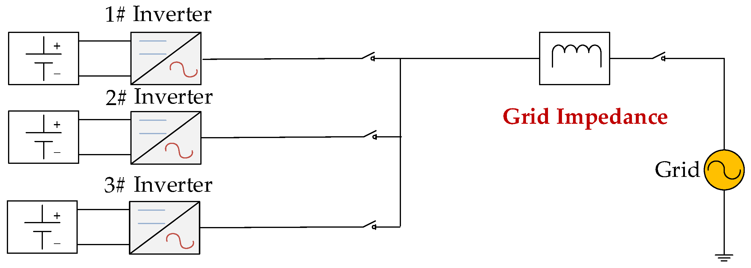
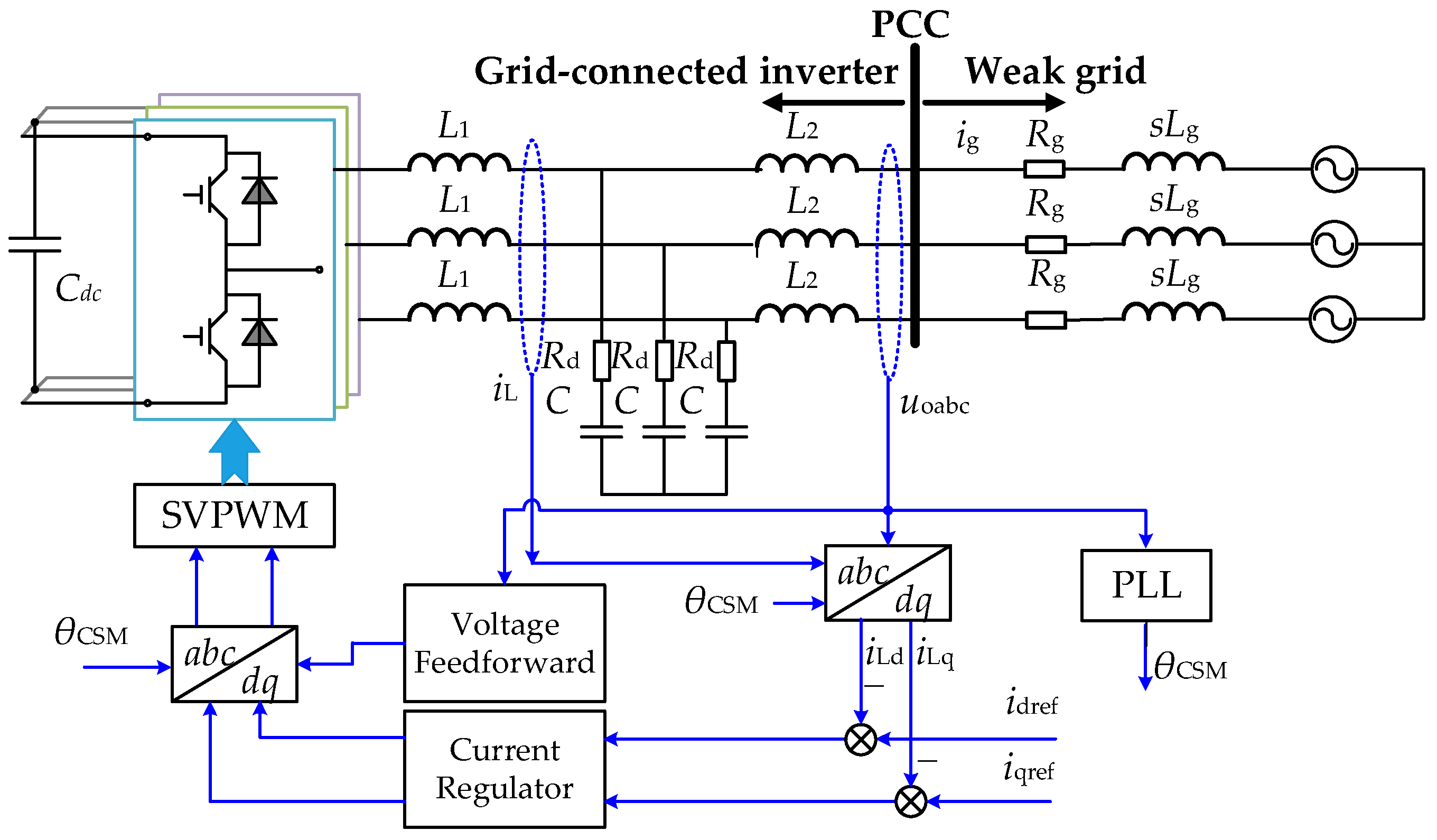
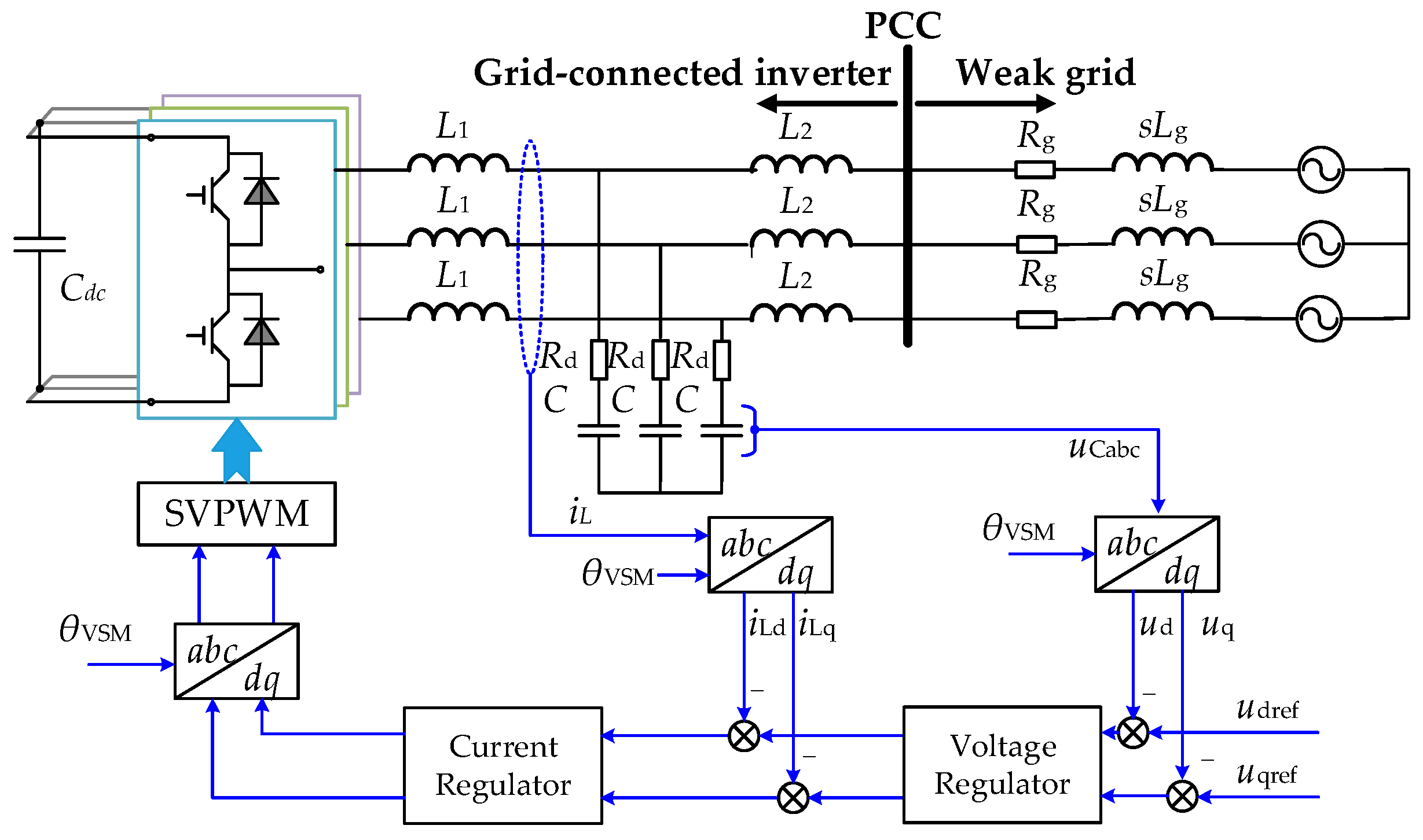
According to the above introduction, the multi-inverter system often operates under a single-mode control strategy with CSM. Figure 1 shows a typical structure of the three-phase grid-connected inverter operating at CSM, and N such structures are connected in parallel will form a multi-inverter system.

In Figure 1, V_dc is the DC voltage, L₁ is the inverter side filter inductor, C is the filter capacitor, R_d is the damping resistor, L₂ is the grid side filter inductor, i_L is the inverter side current, i_g represents the grid current, and e_g is the grid voltage. The i_dref and i_qref are the reference values of the d axis and the q axis current, respectively. i_Ld and i_Lq are the d axis and q axis components, respectively, of the current i_L in the synchronous rotating coordinate system. θ_CSM is the phase obtained by the PLL according to the PCC voltage u_oabc. Z_g is the grid impedance, as shown in Equation (1).

$$Z_{\mathrm{g}}\left(s\right)=R_{\mathrm{g}}+s{L}_{\mathrm{g}}$$

(1)

where R_g and L_g represent the resistive component and inductive component of grid impedance, respectively. Since the stability of the inverter in a weak grid is very susceptible to the inductance component, and the resistive component has the effect of enhancing the stability of the inverter [20], this paper takes R_g = 0.

According to Figure 1, the control block diagram of an inverter operating in CSM is shown in Figure 2. Since the d-axis and q-axis controls are the same, the subscripts d and q are omitted in the following text.

In Figure 2, the G_d(s) represents the influence of the sampler and the delays caused by a digital controller in the s-domain. According to [4,21], the transfer function of the delays incurred by the sampler is expressed as 1/T_s, where T_s is the sampling period. The delays incurred by a digitally controlled system contain the computation delay and the pulse width modulation (PWM) control delay. The expression of G_d(s) is:

$$G_{\mathrm{d}}\left(s\right)=\frac{1}{T_{\mathrm{s}}}\cdot e^{-s{T}_{\mathrm{d}}}\cdot \frac{1-e^{-s{T}_{\mathrm{s}}}}{s}{k}_{\mathrm{PWM}}\approx k_{\mathrm{PWM}}{e}^{-1.5s{T}_{\mathrm{s}}}$$

(2)

where T_d is the delay time.

From Figure 2, the transfer function between the input current command i_ref(s) and the output current i_g(s) can be obtained:

$$i_{\mathrm{g}}\left(s\right)=\frac{i_{\mathrm{ref}}\left(s\right)\cdot PI\left(s\right)\cdot G_{\mathrm{d}}\left(s\right)-e_{\mathrm{g}}\left(s\right)\cdot \left(\begin{array}{l}{s}^2{L}_{1}C/\left(1+R_{\mathrm{d}}Cs\right)+sC/\left(1+R_{\mathrm{d}}Cs\right)\cdot PI\left(s\right)\cdot G_{\mathrm{d}}\left(s\right)\\ -G_{\mathrm{d}}\left(s\right)/k_{\mathrm{PWM}}+1\end{array}\right)}{\left[\begin{array}{l}{s}^3{L}_{1}C/\left(1+R_{\mathrm{d}}Cs\right)\left(L_2+L_g\right)+s^{2}C/\left(1+R_{\mathrm{d}}Cs\right)\left(L_2+L_g\right)PI\left(s\right)\cdot G_{\mathrm{d}}\left(s\right)\\ +s\left(L_1+L_2+L_{\mathrm{g}}\right)+PI\left(s\right)\cdot G_{\mathrm{d}}\left(s\right)-s{L}_{\mathrm{g}}{G}_{\mathrm{d}}\left(s\right)/k_{\mathrm{PWM}}\end{array}\right]}$$

(3)

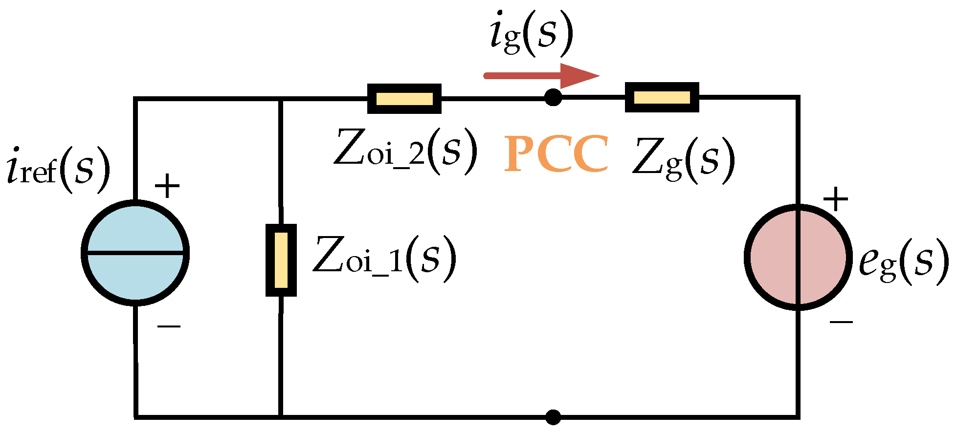
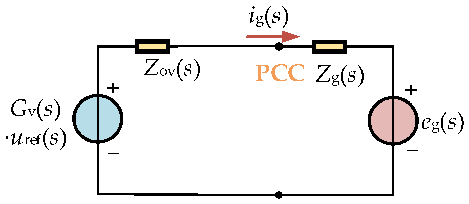
According to [19], the inverter operating in CSM is equivalent to the current source, and from Equation (3), the current source equivalent model is shown in Figure 3.

Z_{oi_1}(s) and Z_{oi_2}(s) in Figure 3 can be derived from Equation (3):

$$Z_{\mathrm{oi}\_1}\left(s\right)=\frac{PI\left(s\right)G_{\mathrm{d}}\left(s\right)}{s^2{L}_{1}C/\left(1+R_{\mathrm{d}}Cs\right)+sC/\left(1+R_{\mathrm{d}}Cs\right)PI\left(s\right)G_{\mathrm{d}}\left(s\right)+1-G_{\mathrm{d}}\left(s\right)}$$

(4)

$$Z_{\mathrm{oi}\_2}\left(s\right)=\frac{s{L}_1}{s^2{L}_{1}C/\left(1+R_{\mathrm{d}}Cs\right)+sC/\left(1+R_{\mathrm{d}}Cs\right)PI\left(s\right)G_{\mathrm{d}}\left(s\right)+1-G_{\mathrm{d}}\left(s\right)}+s{L}_2$$

(5)

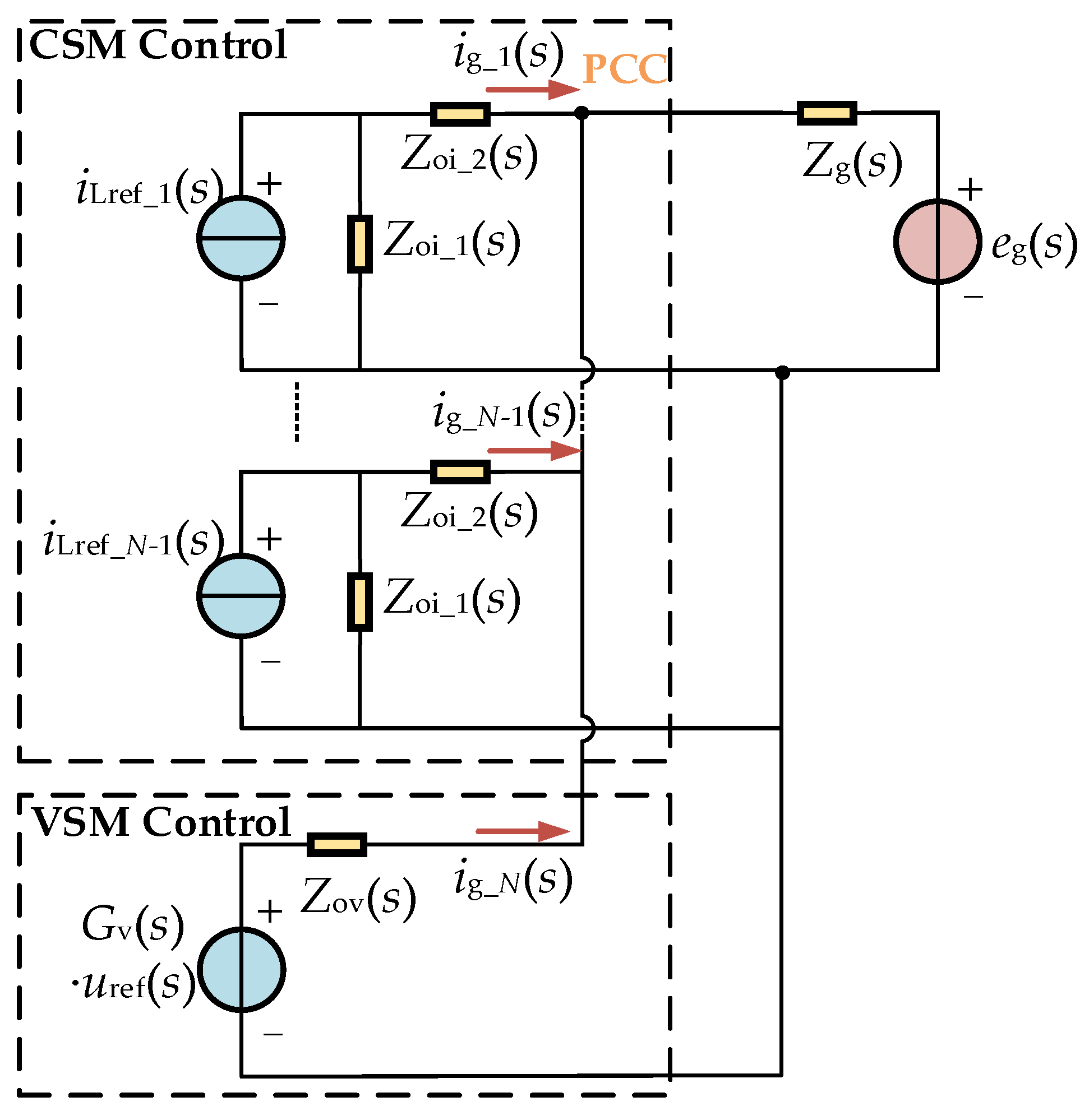
Generally, photovoltaic and wind power plants employ the same type of the inverter with identical hardware parameters and control algorithms, so the equivalent models of the inverter circuits are consistent. According to Figure 3, an equivalent model of a multi-inverter system with CSM-only control is available, as shown in Figure 4. N represents the number of inverters; for a multi-inverter system, N is larger than 2. i represents any inverter in this system, and 1 ≤ i ≤ N.

From Figure 4, we can get:

$$\left[\begin{array}{c}{i}_{\mathrm{g}\_1}\left(s\right)\\ ⋮\\ i_{\mathrm{g}\_i}\left(s\right)\\ ⋮\\ i_{\mathrm{g}\_N}\left(s\right)\end{array}\right]=\left[\begin{array}{ccccc}{G}_{\mathrm{CSM}\_\mathrm{P}}\left(s\right)& \cdots & G_{\mathrm{CSM}\_\mathrm{N}}\left(s\right)& \cdots & G_{\mathrm{CSM}\_\mathrm{N}}\left(s\right)\\ ⋮& \ddots & & & ⋮\\ G_{\mathrm{CSM}\_\mathrm{N}}\left(s\right)& \cdots & G_{\mathrm{CSM}\_\mathrm{P}}\left(s\right)& \cdots & G_{\mathrm{CSM}\_\mathrm{N}}\left(s\right)\\ ⋮& & & \ddots & ⋮\\ G_{\mathrm{CSM}\_\mathrm{N}}\left(s\right)& \cdots & G_{\mathrm{CSM}\_\mathrm{N}}\left(s\right)& \cdots & G_{\mathrm{CSM}\_\mathrm{P}}\left(s\right)\end{array}\right]\left[\begin{array}{c}{i}_{\mathrm{ref}\_1}\left(s\right)\\ ⋮\\ i_{\mathrm{ref}\_i}\left(s\right)\\ ⋮\\ i_{\mathrm{ref}\_N}\left(s\right)\end{array}\right]+G_{\mathrm{CCM}\_\mathrm{E}}\left(s\right)E\left(s\right)$$

(6)

where

$$G_{\mathrm{CCM}\_\mathrm{P}}\left(s\right)=\frac{Z_{\mathrm{oi}\_1}\left(s\right)}{Z_{\mathrm{oi}\_1}\left(s\right)+Z_{\mathrm{oi}\_2}\left(s\right)+Z_{\mathrm{g}}\left(s\right)//\left(\frac{Z_{\mathrm{oi}\_1}\left(s\right)+Z_{\mathrm{oi}\_2}\left(s\right)}{N-1}\right)}$$

(7)

$$G_{\mathrm{CCM}\_\mathrm{N}}\left(s\right)=\frac{Z_{\mathrm{oi}\_1}\left(s\right)\frac{Z_{\mathrm{g}}\left(s\right)}{\left(N-1\right)Z_{\mathrm{g}}\left(s\right)+Z_{\mathrm{oi}\_1}\left(s\right)+Z_{\mathrm{oi}\_2}\left(s\right)}}{Z_{\mathrm{oi}\_1}\left(s\right)+Z_{\mathrm{oi}\_2}\left(s\right)+Z_{\mathrm{g}}\left(s\right)//\left(\frac{Z_{\mathrm{oi}\_1}\left(s\right)+Z_{\mathrm{oi}\_2}\left(s\right)}{N-1}\right)}$$

(8)

$$G_{\mathrm{CCM}\_\mathrm{E}}\left(s\right)=\frac{1}{N{Z}_{\mathrm{g}}\left(s\right)+Z_{\mathrm{oi}\_1}\left(s\right)+Z_{\mathrm{oi}\_2}\left(s\right)}$$

(9)

In Equations (7) and (8), “//” represents the parallel operation, i.e., x//y = xy/(x + y).

3. Stability Analysis of a CSM-Only-Controlled Multi-Inverter System in a Weak Grid

According to Equation (6), due to the existence of grid impedance, multiple coupling transfer functions exist in multi-inverter systems, which affects the system stability. To illustrate the effect of grid impedance on this multi-inverter system, the main parameters of the inverter operating in CSM are given in

Table 1. The main parameters of the inverter operating in current source mode (CSM).

Hardware Parameters of Inverter
Parameters	Value
Inverter capacity	100 kW
Inverter voltage and frequency	380 V, 50 Hz
DC voltage	Vdc = 600 V
LCL filter	L1 = 0.56 mH, C = 90 μF, Rd = 0.5 Ω, L2 = 0.09 mH
Switching frequency	10 kHz
Reference value of grid impedance	Zg(s) = 0.25 mH = 1 p.u.
Controller Parameters of Inverter Operating in CSM
Parameters	Value
Current PI regulator	PI(s) = 1.5 + 500/s
PWM gain	kPWM = 1
Sampling time	Ts = 1 ms
Delay function	Gd(s) = kPWM∙e−s*1.5*Ts = e−s*1.5*0.001

PWM: pulse width modulation.

.

In this section, the multi-inverter system takes the number of units N = 3 as an example and takes the output current of the first inverter (i = 1) as the research object, and the characteristics of the transfer functions G_{CSM_P}(s), G_{CSM_N}(s), and G_{CSM_E}(s) are studied, respectively.

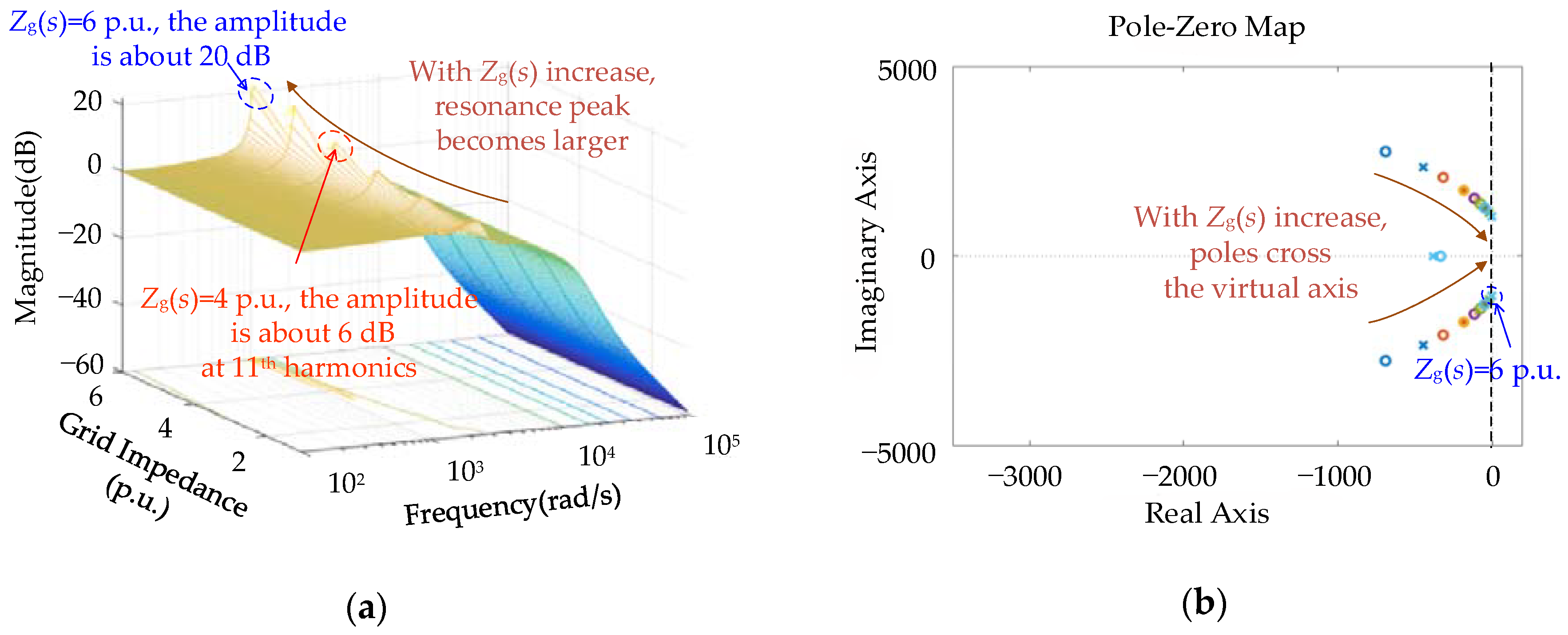
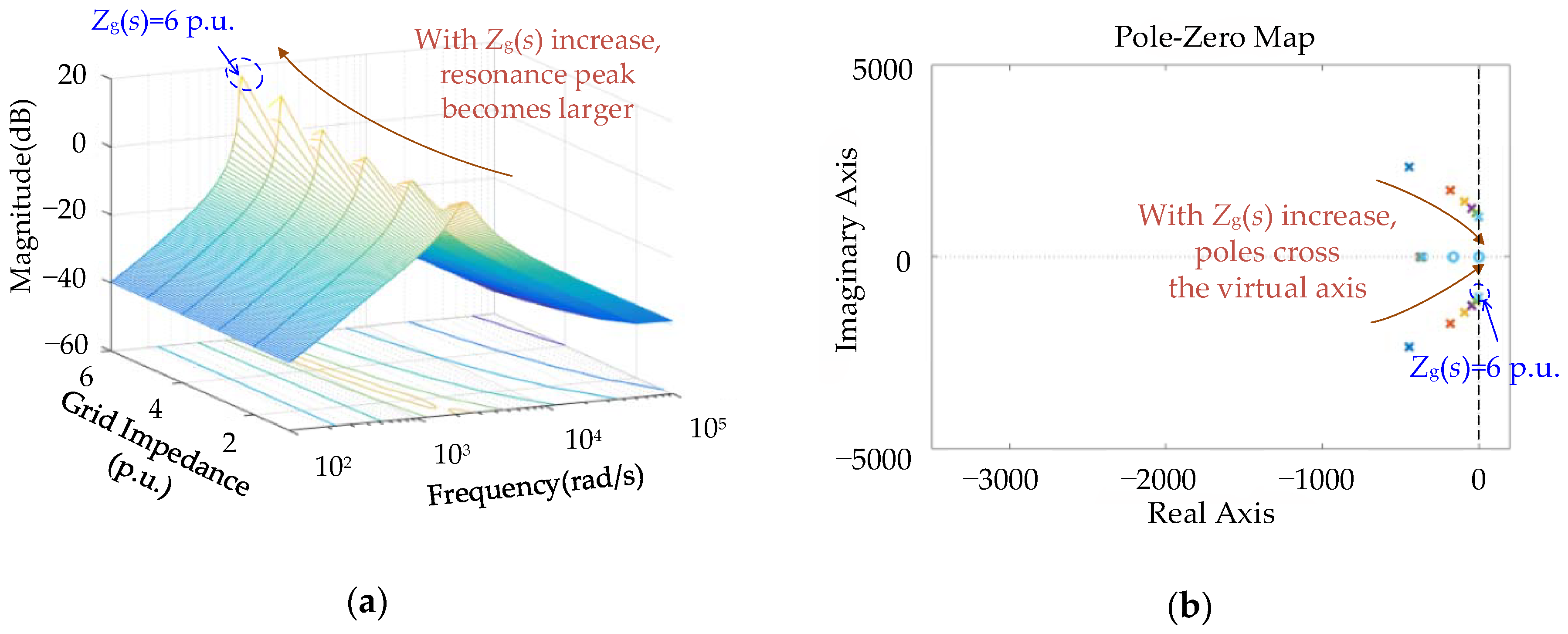
G_{CSM_P}(s) represents the closed-loop transfer function of the reference current to the output current of the CSM-controlled inverters. The Bode diagram and pole-zero map of G_{CSM_P}(s) with the grid impedance Z_g(s) changes from 1 p.u. to 6 p.u. are shown in Figure 5a and Figure 5b, respectively. From Figure 5a, when the grid impedance increases, the amplitude of the resonance peak gets larger, and its frequency is gradually moving toward the low-frequency direction. When Z_g(s) = 6 p.u., the amplitude of the resonance peak is nearly 20 dB, which means that the current harmonics here will be amplified about 10 times, and the output current will resonate. To further illustrate the stability issue, the distribution of poles near the imaginary axis is given in Figure 5b. With a Z_g(s) increase from 1 p.u. to 6 p.u., the poles gradually cross the imaginary axis, so the inverter will operate in an unstable fashion.

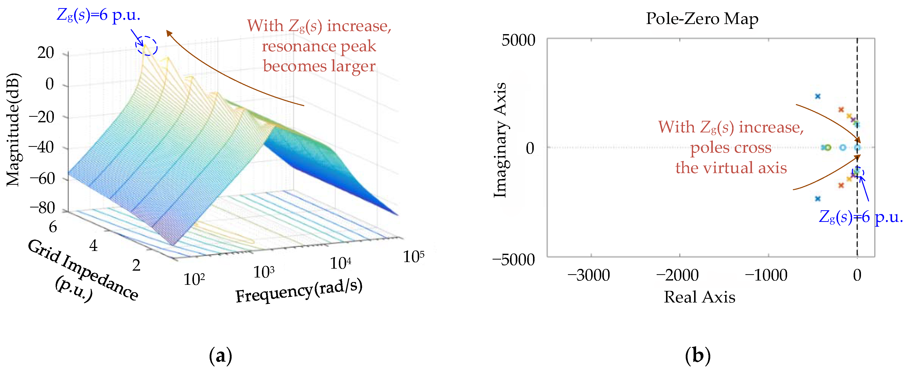
G_{CSM_N}(s) represents the interaction between the CSM-controlled inverters. The Bode diagram and pole-zero map of G_{CSM_N}(s) with the grid impedance Z_g(s) changes from 1 p.u. to 6 p.u. are shown in Figure 6a and Figure 6b, respectively. From Figure 6a, when the grid impedance increases, the amplitude of the resonance peak appears and becomes larger. When Z_g(s) = 6 p.u., the amplitude of resonance peak is nearly 20 dB at 1000 rad/s, which means that the current harmonics of one inverter will be amplified in another inverter by about 10 times. Therefore, with the increase of grid impedance, the coupling between the inverters increases, and the harmonics of the other inverters will be amplified and become resonant at the output current of other inverters. To further illustrate the stability issue, the distribution of poles near the imaginary axis is shown in Figure 6b. With the Z_g(s) increase from 1 p.u. to 6 p.u., the poles gradually cross the imaginary axis, so the inverter will operate in an unstable fashion.

G_{CSM_E}(s) represents the impact between the CSM-controlled inverters and the grid. The Bode diagram and pole-zero map of G_{CSM_E}(s) with the grid impedance Z_g(s) changes from 1 p.u. to 6 p.u. are shown in Figure 7a and Figure 7b, respectively. Comparing Figure 6 and Figure 7, it can be seen that the Bode diagram and the pole-zero map of the transfer function are very similar, so there is a similar conclusion: with the grid impedance increases, the degree of coupling between the grid and the inverter increases, and the background harmonics of the weak grid will be amplified and become resonant at the output current of the inverter.

In summary, by constructing the closed-loop transfer function model of the multi-inverter system with CSM-only control, it is found that as the grid impedance increases, a resonance peak appears and the degree of coupling between the inverters and the grid increases, and the inverter is prone to output current resonance.

4. Proposed Dual-Mode Control Strategy in the Weak Grid

Previous research [19] points out that the grid-connected inverter operating in VSM is more stable in a weak grid than CSM. Due to the object of analysis in this study being only a single inverter, if the inverters in a multi-inverter system are equipped with such a dual-mode adaptive switching operation control strategy which could adaptively switch the operating mode between CSM and VSM, then a novel control strategy for multi-inverter system stability based on dual mode grid impedance adaptation in the weak grid is proposed: One inverter operating in CSM in the system could switch to VSM control based on the grid impedance identification, and then the multi-inverter system will run under dual-mode control and operate stably.

In order to validate this proposed control strategy, similar to the above analysis in Section 2, the model of a multi-inverter system with dual modes is established.

Figure 8 shows a typical structure of the three-phase grid-connected inverter operating in VSM. The main circuit of the inverter is the same as that of Figure 1. u_dref and u_qref are the d-axis and q-axis components of the reference voltage loop, respectively. θ_VSM is the phase of the power angle which can be set according to the desired output power. The u_d and u_q are the d-axis and q-axis components of the capacitor voltage u_Cabc, respectively. Differently from CSM control, the inverter operating in VSM is equivalent to a voltage source.

According to Figure 8, the control block diagram of the inverter operating in VSM is shown in Figure 9.

In Figure 9, the PI_v(s) represents the voltage outer loop proportional-integral (PI) regulator, and PI_c(s) is the current inner loop proportional regulator. The expressions of PI_v(s) and PI_c(s) are shown as follows:

$$P{I}_{\mathrm{v}}\left(s\right)=K_{\mathrm{vP}}+\left(K_{\mathrm{vI}}/s\right)$$

(10)

$$P{I}_{\mathrm{c}}\left(s\right)=K_{\mathrm{iP}}$$

(11)

where K_vP and K_vI are proportional and integral coefficients of the PI_v(s), respectively. K_iP is the proportional coefficient of the PI_c(s).

According to Figure 9, the transfer function between the input voltage command u_ref(s) and the output voltage u(s) can be obtained [22]:

$$\begin{array}{l}u\left(s\right)=u_{\mathrm{ref}}\left(s\right)\frac{P{I}_{\mathrm{v}}\left(s\right)}{P{I}_{\mathrm{v}}\left(s\right)\cdot P{I}_{\mathrm{c}}\left(s\right)G_{\mathrm{d}}\left(s\right)+sC/\left(1+R_{\mathrm{d}}Cs\right)\left(s{L}_1+P{I}_{\mathrm{c}}\left(s\right)G_{\mathrm{d}}\left(s\right)\right)+1}\\ -i_{\mathrm{g}}\left(s\right)\left(\frac{s{L}_1+P{I}_{\mathrm{c}}\left(s\right)G_{\mathrm{d}}\left(s\right)}{P{I}_{\mathrm{v}}\left(s\right)\cdot P{I}_{\mathrm{c}}\left(s\right)G_{\mathrm{d}}\left(s\right)+sC/\left(1+R_{\mathrm{d}}Cs\right)\left(s{L}_1+P{I}_{\mathrm{c}}\left(s\right)G_{\mathrm{d}}\left(s\right)\right)+1}+s{L}_2\right)\end{array}$$

(12)

From Equation (12), the voltage source equivalent model is shown in Figure 10; G_v(s) and Z_ov(s) in Figure 10 can be derived from Equation (12):

$$G_{\mathrm{v}}\left(s\right)=\frac{P{I}_{\mathrm{v}}\left(s\right)}{P{I}_{\mathrm{v}}\left(s\right)\cdot P{I}_{\mathrm{c}}\left(s\right)G_{\mathrm{d}}\left(s\right)+sC/\left(1+R_{\mathrm{d}}Cs\right)\left(s{L}_1+P{I}_{\mathrm{c}}\left(s\right)G_{\mathrm{d}}\left(s\right)\right)+1}$$

(13)

$$Z_{\mathrm{ov}}\left(s\right)=\frac{s{L}_1+P{I}_{\mathrm{c}}\left(s\right)G_{\mathrm{d}}\left(s\right)}{P{I}_{\mathrm{v}}\left(s\right)\cdot P{I}_{\mathrm{c}}\left(s\right)G_{\mathrm{d}}\left(s\right)+sC/\left(1+R_{\mathrm{d}}Cs\right)\left(s{L}_1+P{I}_{\mathrm{c}}\left(s\right)G_{\mathrm{d}}\left(s\right)\right)+1}+s{L}_2$$

(14)

4.1. Modeling of the Multi-Inverter System with Dual Modes

According to Figure 3 and Figure 10, when the multi-inverter system contains CSM- and VSM-controlled inverters at the same time, the equivalent model of a multi-inverter system with dual modes is shown in Figure 11.

From Figure 11, we can get:

$$\begin{array}{l}\left[\begin{array}{c}{i}_{\mathrm{g}\_1}\left(s\right)\\ ⋮\\ i_{\mathrm{g}\_i}\left(s\right)\\ ⋮\\ i_{\mathrm{g}\_N-1}\left(s\right)\end{array}\right]=\left[\begin{array}{ccccc}{G}_{\mathrm{VSM}\_\mathrm{P}}\left(s\right)& \cdots & G_{\mathrm{VSM}\_\mathrm{N}}\left(s\right)& \cdots & G_{\mathrm{VSM}\_\mathrm{N}}\left(s\right)\\ ⋮& \ddots & & & ⋮\\ G_{\mathrm{VSM}\_\mathrm{N}}\left(s\right)& \cdots & G_{\mathrm{VSM}\_\mathrm{P}}\left(s\right)& \cdots & G_{\mathrm{VSM}\_\mathrm{N}}\left(s\right)\\ ⋮& & & \ddots & ⋮\\ G_{\mathrm{VSM}\_\mathrm{N}}\left(s\right)& \cdots & G_{\mathrm{VSM}\_\mathrm{N}}\left(s\right)& \cdots & G_{\mathrm{VSM}\_\mathrm{P}}\left(s\right)\end{array}\right]\left[\begin{array}{c}{i}_{\mathrm{ref}\_1}\left(s\right)\\ ⋮\\ i_{\mathrm{ref}\_i}\left(s\right)\\ ⋮\\ i_{\mathrm{ref}\_N-1}\left(s\right)\end{array}\right]\\ +G_{\mathrm{VSM}\_\mathrm{E}}\left(s\right)e_{\mathrm{g}}\left(s\right)+G_{\mathrm{VSM}\_\mathrm{U}}\left(s\right)u_{\mathrm{ref}}\left(s\right)\end{array}$$

(15)

where

$$G_{\mathrm{VCM}\_\mathrm{P}}\left(s\right)=\frac{Z_{\mathrm{oi}\_1}\left(s\right)}{Z_{\mathrm{oi}\_1}\left(s\right)+Z_{\mathrm{oi}\_2}\left(s\right)+Z_{\mathrm{g}}\left(s\right)//\left(\frac{Z_{\mathrm{oi}\_1}\left(s\right)+Z_{\mathrm{oi}\_2}\left(s\right)}{N-2}\right)//Z_{\mathrm{ov}}\left(s\right)}$$

(16)

$$G_{\mathrm{VCM}\_\mathrm{N}}\left(s\right)=\frac{-Z_{\mathrm{oi}\_1}\left(s\right)\left(\frac{Z_{\mathrm{g}}\left(s\right)}{Z_{\mathrm{oi}\_1}\left(s\right)+Z_{\mathrm{oi}\_2}\left(s\right)+\left(N-2\right)Z_{\mathrm{g}}\left(s\right)}//Z_{\mathrm{ov}}\left(s\right)\right)}{Z_{\mathrm{oi}\_1}\left(s\right)+Z_{\mathrm{oi}\_2}\left(s\right)+Z_{\mathrm{g}}\left(s\right)//\left(\frac{Z_{\mathrm{oi}\_1}\left(s\right)+Z_{\mathrm{oi}\_2}\left(s\right)}{N-2}\right)//Z_{\mathrm{ov}}\left(s\right)}$$

(17)

$$G_{\mathrm{VCM}\_\mathrm{E}}\left(s\right)=-\frac{Z_{\mathrm{ov}}\left(s\right)}{\left(Z_{\mathrm{g}}\left(s\right)+Z_{\mathrm{ov}}\left(s\right)\right)\left(Z_{\mathrm{oi}\_1}\left(s\right)+Z_{\mathrm{oi}\_2}\left(s\right)\right)+\left(N-1\right)Z_{\mathrm{ov}}\left(s\right)Z_{\mathrm{g}}\left(s\right)}$$

(18)

$$G_{\mathrm{VCM}\_\mathrm{U}}\left(s\right)=-\frac{Z_{\mathrm{g}}\left(s\right)G_{\mathrm{v}}\left(s\right)}{\left(Z_{\mathrm{g}}\left(s\right)+Z_{\mathrm{ov}}\left(s\right)\right)\left(Z_{\mathrm{oi}\_1}\left(s\right)+Z_{\mathrm{oi}\_2}\left(s\right)\right)+\left(N-1\right)Z_{\mathrm{ov}}\left(s\right)Z_{\mathrm{g}}\left(s\right)}$$

(19)

In Equations (16) and (17), “//” represents the parallel operation, i.e., x//y = xy/(x + y).

4.2. Stability Analysis of the Multi-Inverter System with Dual Modes

In Section 2, the stability of the multi-inverter system with CSM-only control is analyzed; a similar analysis method will be used in this section to verify that the proposed dual-mode multi-inverter system can effectively improve system stability and reduce coupling between inverters in a weak grid.

The main parameters of the inverter operating in VSM are given in

Table 2. The main parameters of the inverter operating in voltage source mode (VSM).

Controller Parameters of Inverter Operating in VSM
Parameters	Value
Voltage PI regulator	PIv(s) = 1500 + 1/s
Current proportional regulator	PIc(s) = 10
PWM gain	kPWM = 1
Sampling time	Ts = 1 ms
Delay function	Gd(s) = kPWM∙e−s*1.5*Ts = e−s*1.5*0.001

. It is worth mentioning that the hardware parameters of the VSM-controlled inverter are consistent with the CSM. Therefore, Table 2 only gives the corresponding controller parameters.

In this section, the multi-inverter system takes the number of units N = 3 as an example. This system consists of two CSM-controlled inverters and one VSM-controlled inverter to form a dual-mode hybrid system. Moreover, according to reference [19], grid-connected inverters running in VSM can operate stably in a weak grid with high grid impedance, while grid-connected inverters in CSM are prone to output current resonance. Therefore, the stability of this dual-mode multi-inverter system is studied from the point of view of a CSM-controlled inverter in this paper.

In order to correspond to the analysis of Section 2, the output current of the first CSM-controlled inverter (i = 1) in the multi-inverter system is also taken as the research object, and the characteristics of the transfer functions G_{VSM_P}(s), G_{VSM_N}(s), G_{VSM_E}(s), and G_{VSM_U}(s) are studied, respectively.

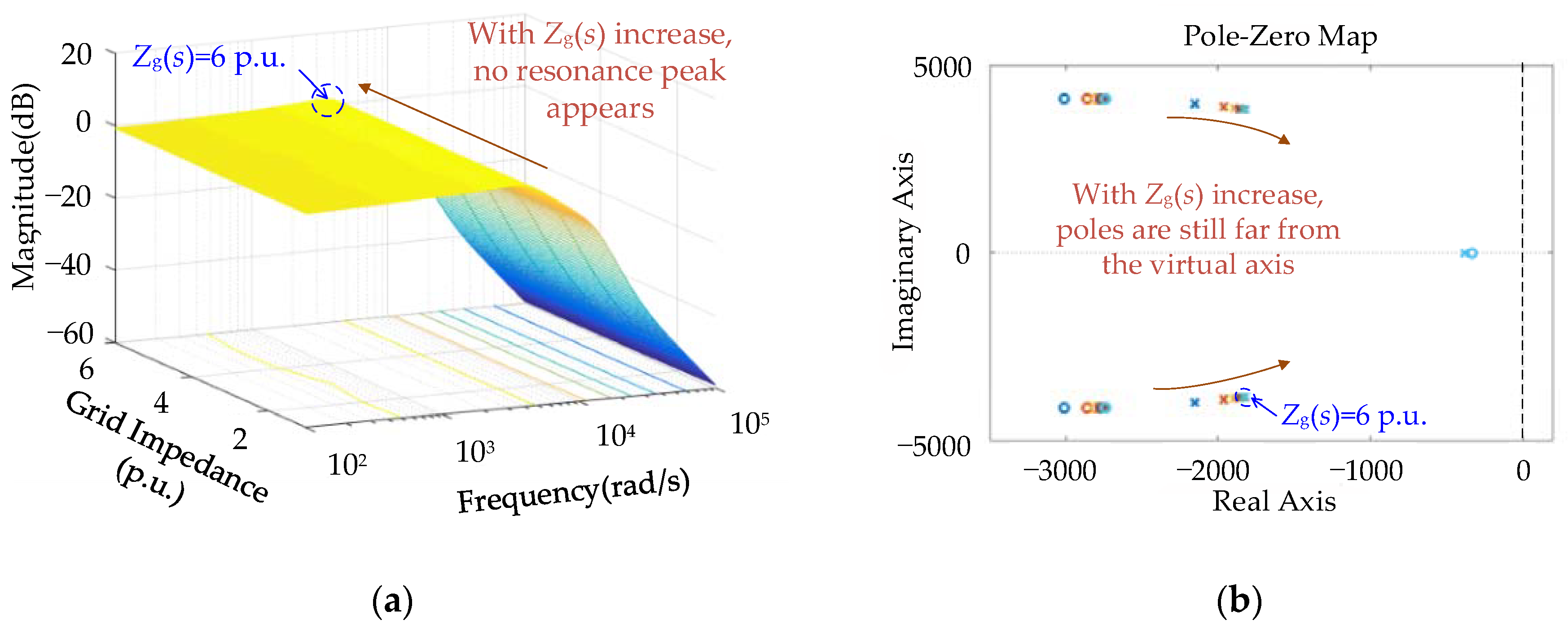
Similar to the multi-inverter system with CSM-only control, G_{VSM_P}(s) represents the closed-loop transfer function of the reference current to the output current of the CSM-controlled inverters in the dual-mode controlled multi-inverter system. The Bode diagram and pole-zero map of G_{VSM_P}(s) with the grid impedance Z_g(s) changes from 1 p.u. to 6 p.u. are shown in Figure 12a and Figure 12b, respectively. Differently from Figure 5, with the increase of grid impedance, the output current of the grid-connected inverter controlled by the current source has no resonance peak, and the pole is far from the virtual axis. It shows that the inverter can operate stably at this time.

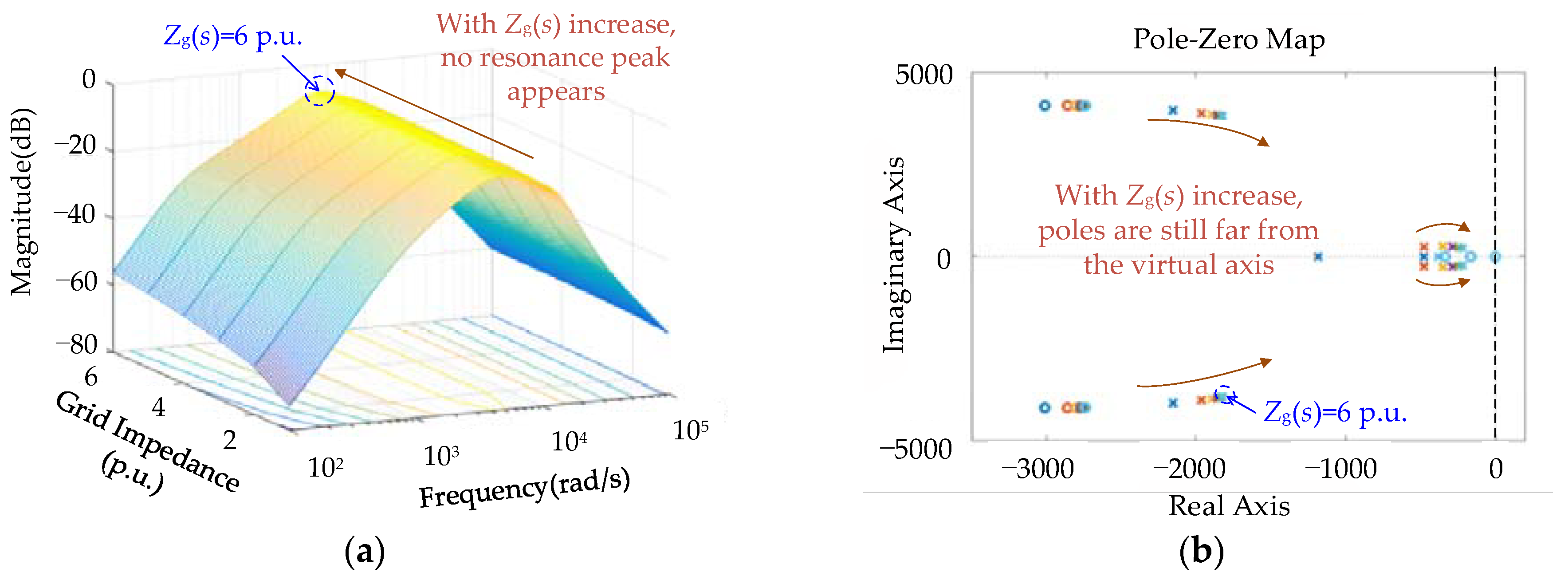
Similarly, G_{VSM_N}(s) represents the interaction between the CSM-controlled inverters. The Bode diagram and pole-zero map of G_{VSM_N}(s) with the grid impedance Z_g(s) changes from 1 p.u. to 6 p.u. are shown in Figure 13a and Figure 13b, respectively. With the increase of grid impedance, the output current of the grid-connected inverter controlled by CSM has no resonance peak and the poles are still far from the virtual axis. Therefore, with the grid impedance increases, the degree of coupling between the inverters does not change significantly.

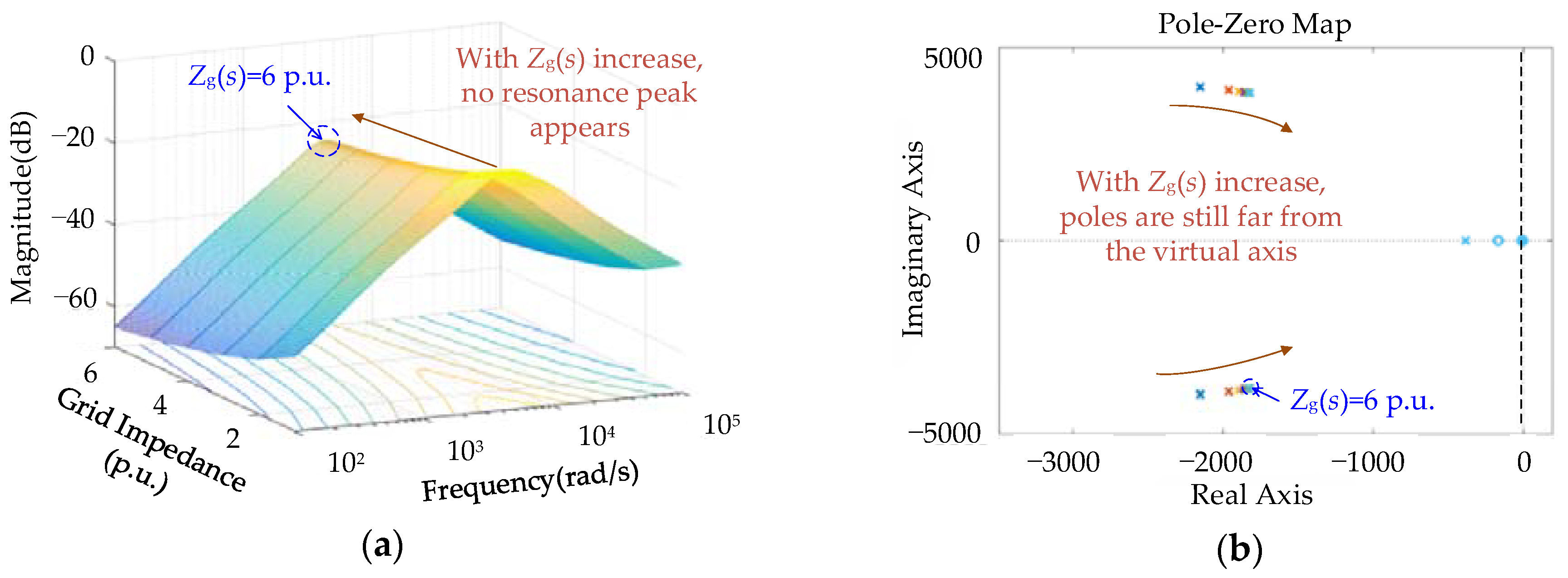
Similarly, G_{VSM_E}(s) represents the coupling degree between the CSM-controlled inverters and grid. The Bode diagram and pole-zero map of G_{VSM_E}(s) with the grid impedance Z_g(s) changes from 1 p.u. to 6 p.u. are shown in Figure 14a and Figure 14b, respectively. With the increase of grid impedance, the output current of the grid-connected inverter controlled by CSM has no resonance peak and the poles are still far from the virtual axis. Therefore, as the grid impedance increases, the degree of coupling between the inverters and the grid does not have apparent changes.

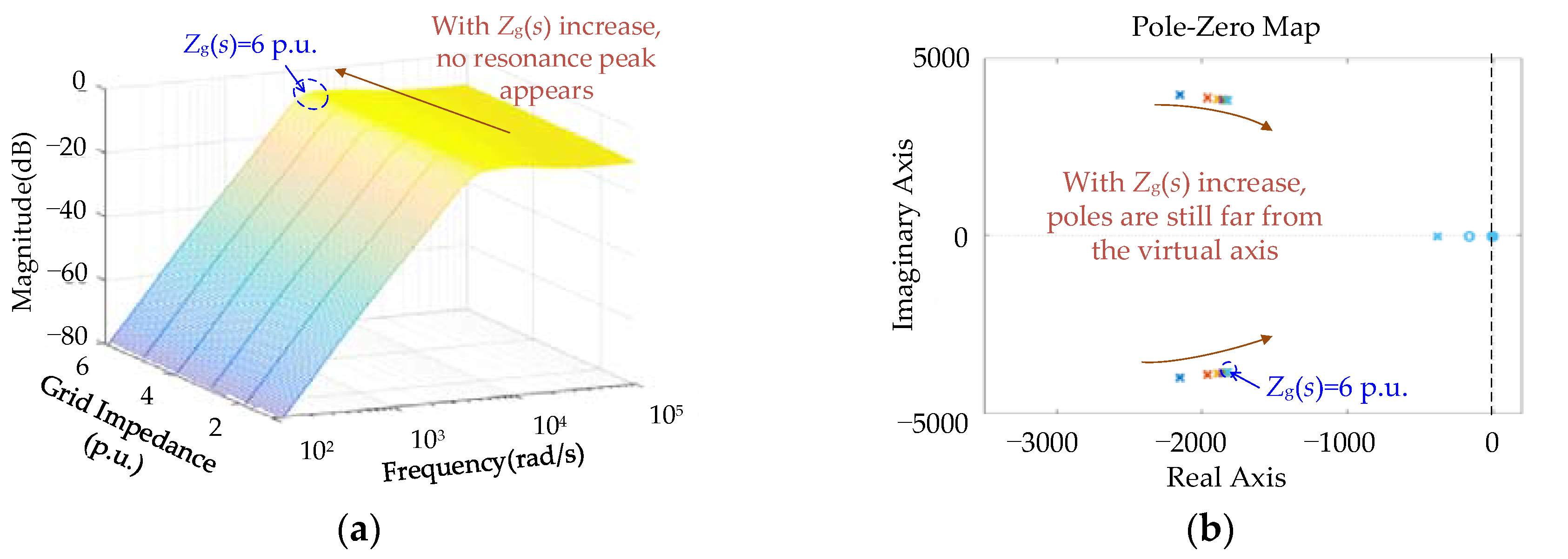
It is worth noting that a new transfer function, G_{VSM_U}(s), appears when the multi-inverter system is operating under the dual-mode control. G_{VSM_U}(s) represents the degree of coupling between the CSM-controlled inverters and the VSM-controlled inverter. The Bode diagram and pole-zero map of G_{VSM_U}(s) with the grid impedance Z_g(s) changes from 1 p.u. to 6 p.u. are shown in Figure 15a and Figure 15b, respectively. It can be seen from Figure 15 that there is no resonance peak on the Bode diagram when the grid impedance increases, and the poles are still far from the virtual axis. Therefore, in this kind of dual-mode multi-inverter system, the coupling between CSM- and VSM-controlled inverters is not increased.

In summary, since the grid-connected inverter operating in voltage source mode (VSM) is more stable in an extremely weak grid than CSM [19], a novel stability improvement strategy of the multi-inverter system in a weak grid utilizing dual-mode control is proposed: one inverter operating in CSM will be alternated into VSM if the grid impedance is high. It is theoretically proved that the coupling between the inverters and the resonance in the output current can be suppressed effectively with the proposed scheme.

5. Simulation and Experimental Results

The proposed dual-mode control strategy in a weak grid is confirmed through Matlab/Simulink and an experiment. Figure 16 shows the multi-inverter system with three parallel grid-connected inverters in a weak grid. The system parameters of the simulation as well as the experiments are almost the same and are enumerated in Table 1 and Table 2.

In Figure 16, the grid impedance is set to Z_g(s) = 4 p.u., and the 3# inverter is equipped with the grid impedance dual-mode strategy, so the inverter can adaptively switch between CSM and VSM according to the grid impedance. Moreover, it can be seen from Figure 5 that when the grid impedance is Z_g(s) = 3 p.u., the amplitude of the resonance peak is about 6 dB; that is, the harmonic will be amplified about two times. 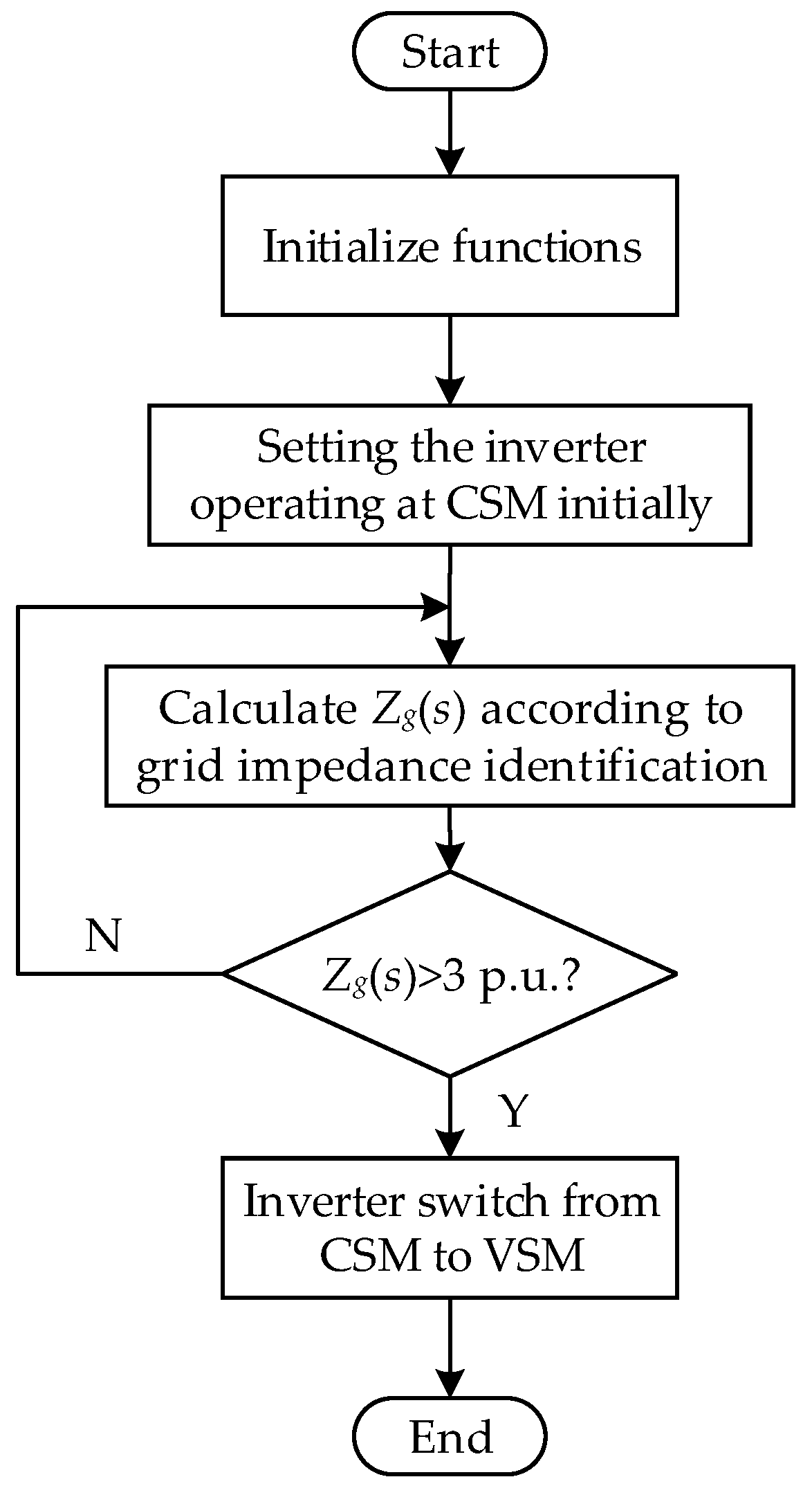Therefore, for the specific parameters of the inverter in this paper, as shown in Table 1 and Table 2, the grid impedance Z_g(s) = 3 p.u. is set to the boundary value of CSM and VSM. Based on this value, Figure 17 shows the flow chart of the switching process between CSM and VSM. Notably, there are many kinds of grid impedance identification schemes [23,24,25,26,27], and the method of single harmonic injection [23] is used in this paper. Since the grid impedance identification scheme is not the core work of this paper, it will not be discussed in this paper.

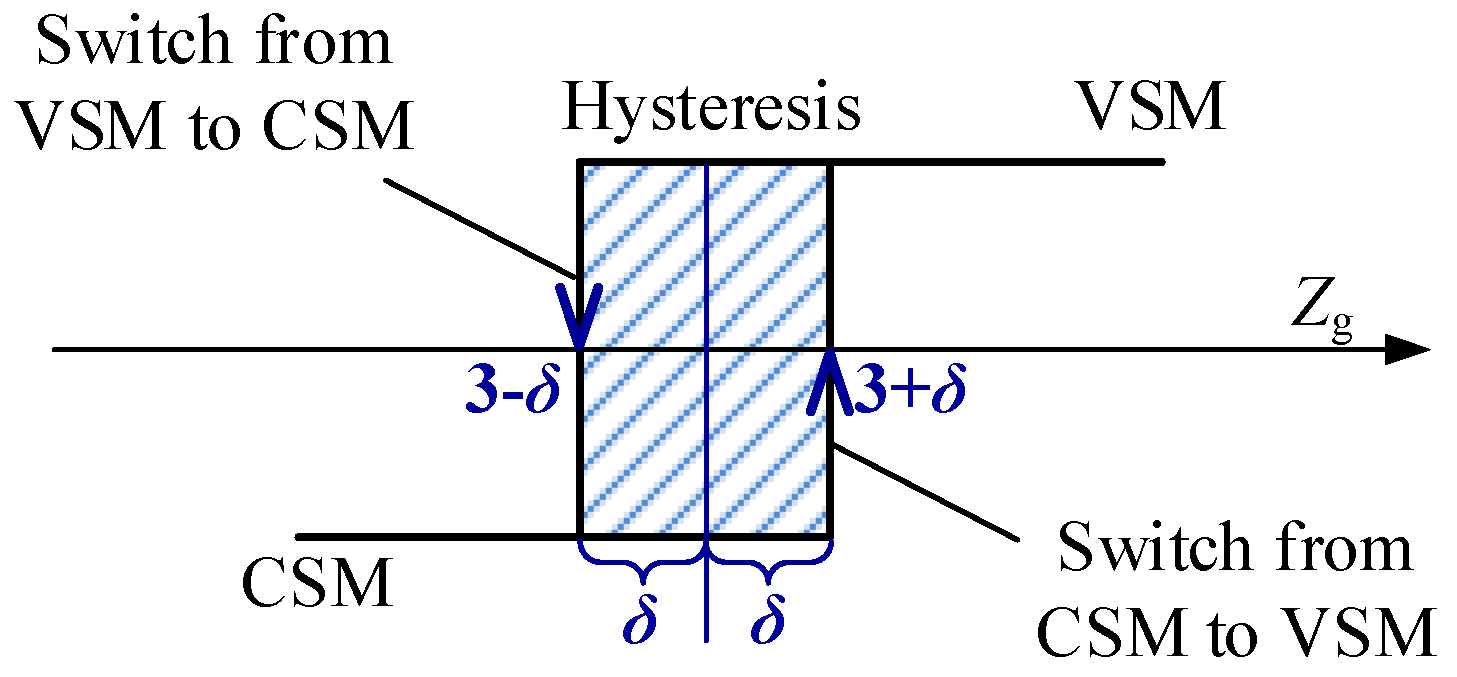
In order to avoid chattering between the two modes, a hysteresis switching process as shown in Figure 18 is used in the actual simulation and experiment. As can be seen from Figure 18, the hysteresis center is set to the boundary value Z_g(s) = 3 p.u., and the hysteresis width is set to δ, where δ = 5% × 3 p.u. = 0.15 p.u.. At this point, the mode switching process of the grid-connected inverter is described as follows: When the grid becomes stronger to weaker, i.e., the grid impedance Z_g(s) > (3 + δ) p.u., the inverter should switch from CSM to VSM; and when the grid becomes weaker to stronger, i.e., the grid impedance Z_g(s) < (3 − δ) p.u., the inverter should switch from VSM to CSM.

5.1. Simulation Verification

The simulation conditions are described as follows:

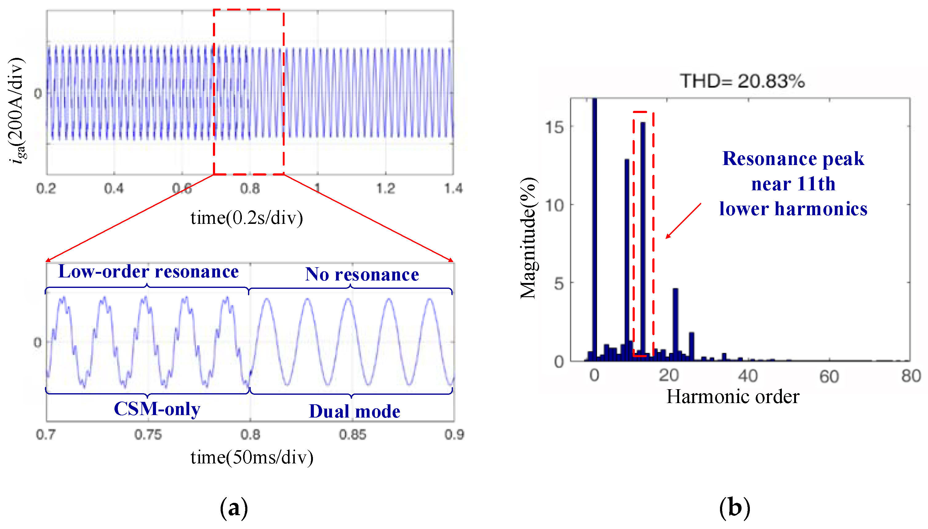
Figure 19a shows the simulation waveform of the A-phase grid current i_ga of the 1# inverter when the multi-inverter system is converted from the original CSM-only control at 0.8 s to the dual-mode control system.

Before 0.8 s, all three inverters in the system are running in CSM. It can be found that the current waveform has obvious low-order resonance before 0.8 s, and Figure 19b shows the spectrum of the A-phase grid current i_ga before 0.8 s. From Figure 19b, the resonance peak is near the 11th harmonics, and this is consistent with the conclusion that when the grid impedance in Figure 5a is Z_g(s) = 4 p.u., and the resonant peak frequency is around the 11th harmonics.

After 0.8 s, due to the 3# inverter in the system having a dual-mode adaptive control algorithm based on the grid impedance added, and since Z_g(s) = 4 p.u. > 3 p.u., it will adaptively switch from CSM control to VSM at 0.8 s. After 0.8 s, it is found that the output current resonance phenomenon disappears remarkably and the output current quality is high.

In summary, it can be seen that the dual-mode multi-inverter control strategy proposed in this paper can effectively suppress the output current resonance phenomenon caused by the grid impedance in the weak grid and improve the stability of the grid-connected inverter system.

5.2. Experimental Verification

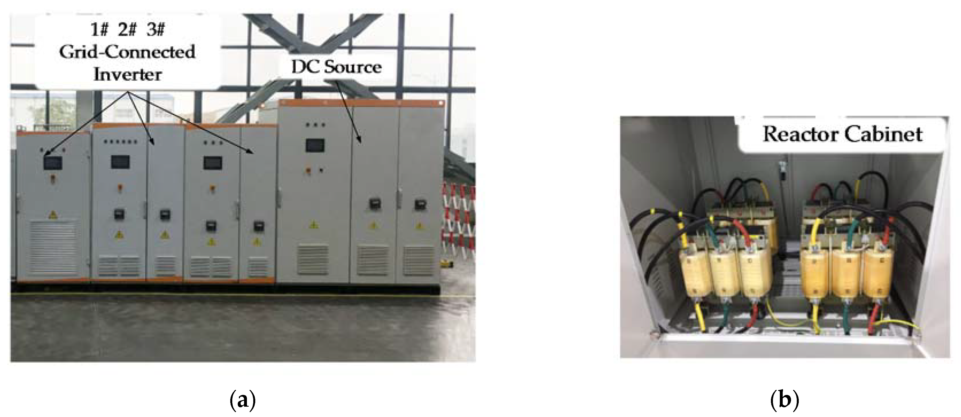
Experiments were also carried out on an experimental platform consisting of three 100-kW grid-connected inverters to verify the proposed control scheme. The control circuit is implemented on a DSP chip TMS320F28335, which implements the proposed control strategies, as described in the previous sections. In the experiments, a three-phase programmable rectifier is used to represent the DC source. The grid impedance is achieved by a series of practical reactors in a reactor cabinet, and the corresponding grid inductance is 0.25 × 4 mH (that is, Z_g(s) = 4 p.u.). The experimental platform is depicted in Figure 20.

Corresponding to the simulation, the experimental conditions are described as follows:

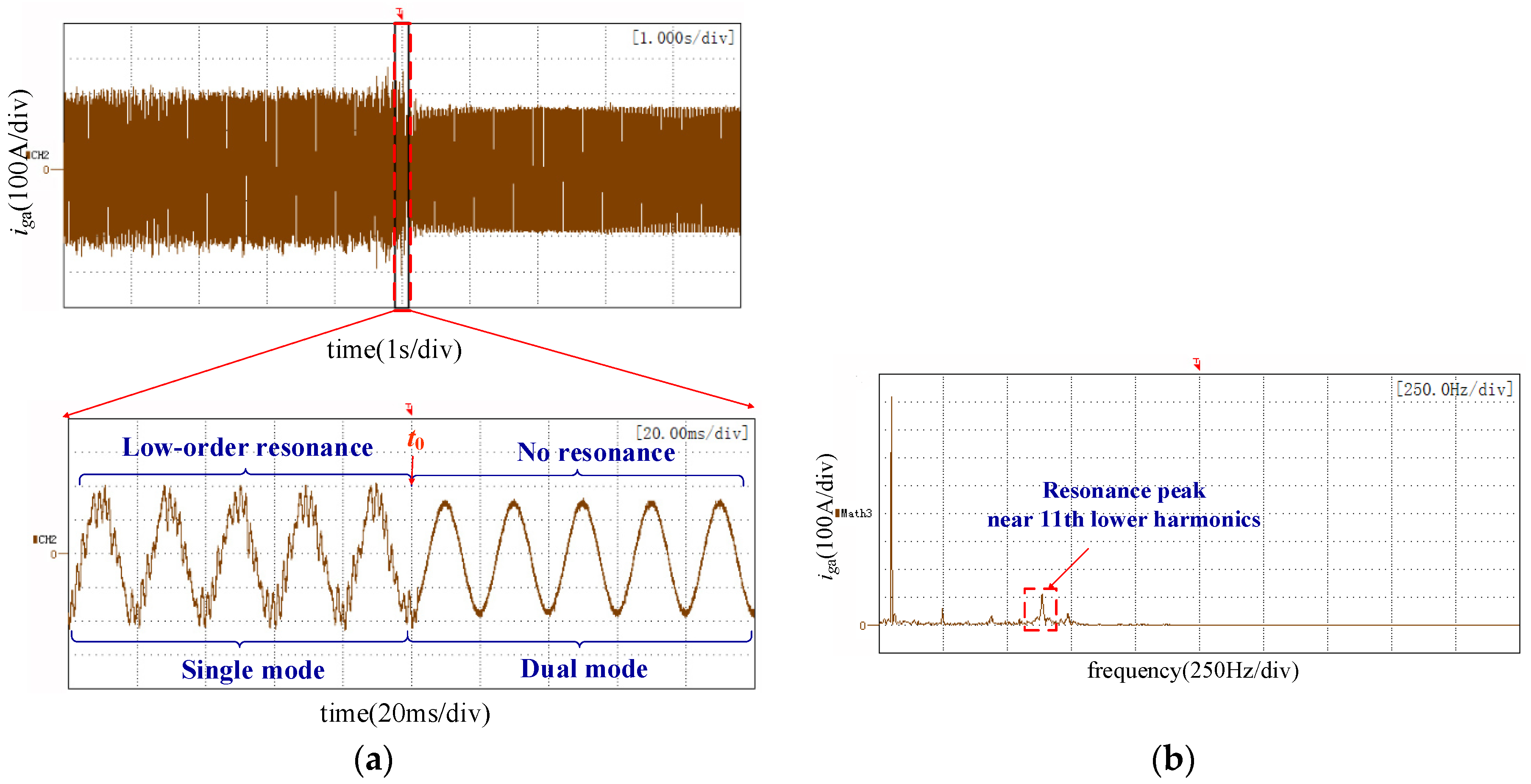
Figure 21a shows the experimental waveform of the A-phase grid current i_ga of the 1# inverter when the multi-inverter system is converted from the original CSM-only control at time t₀ to the dual-mode control system.

Before t₀, all three inverters in the system are running in CSM. Similarly to the simulation results, the current waveform has obvious low-order resonance before 0.8 s, and Figure 21b shows the spectrum of the A-phase grid current i_ga before t₀. From Figure 21b, the resonance peak is near the 11th harmonics, and this is consistent with the conclusion that when the grid impedance in Figure 5a is Z_g(s) = 4 p.u., the resonant peak frequency is around the 11th harmonics.

After t₀, due to the 3# inverter in the system having a dual-mode adaptive control algorithm based on the grid impedance added, and since Z_g(s) = 4 p.u. > 3 p.u., it will adaptively switch from CSM control to VSM at t₀. After t₀, it is found that the output current resonance phenomenon disappears remarkably and the output current quality is high.

It can be concluded from Figure 19 to Figure 21 that the experimental results are in good agreement with the simulation results, and thus the superiority of the proposed control strategy is further verified.

6. Conclusions

In this paper, a closed-loop transfer function model of the multi-inverter system operating in current source mode (CSM) is established, by which it is concluded that output current resonance will occur with the increase in the grid impedance. In order to address this problem, this paper presents a novel dual-mode control scheme of multiple inverters; i.e., one inverter operating in CSM will be alternated into voltage source mode (VSM) if the grid impedance is high. It is theoretically proved that the coupling between the inverters and the resonance in the output current can be suppressed effectively with the proposed scheme. Finally, the validity of the proposed theory is demonstrated by extensive simulations and experiments.