A Physics-Based Electrochemical Model for Lithium-Ion Battery State-of-Charge Estimation Solved by an Optimised Projection-Based Method and Moving-Window Filtering

Abstract

State-of-charge (SOC) is one of the most critical parameters in battery management systems (BMSs). SOC is defined as the percentage of the remaining charge inside a battery to the full charge, and thus ranges from 0% to 100%. This percentage value provides important information to manufacturers about the performance of the battery and can help end-users identify when the battery must be recharged. Inaccurate estimation of the battery SOC may cause over-charge or over-discharge events with significant implications for system safety and reliability. Therefore, it is crucial to develop methods for improving the estimation accuracy of battery SOC. This paper presents an electrochemical model for lithium-ion battery SOC estimation involving the battery’s internal physical and chemical properties such as lithium concentrations. To solve the computationally complex solid-phase diffusion partial differential equations (PDEs) in the model, an efficient method based on projection with optimized basis functions is presented. Then, a novel moving-window filtering (MWF) algorithm is developed to improve the convergence rate of the state filters. The results show that the developed electrochemical model generates 20 times fewer equations compared with finite difference-based methods without losing accuracy. In addition, the proposed projection-based solution method is three times more efficient than the conventional state filtering methods such as Kalman filter.

1. Introduction

The size of the market for lithium-ion (Li-ion) batteries has grown considerably in recent years. According to recent statistics provided by Grand View Research, Inc. (https://www.grandviewresearch.com/), the global Li-ion battery market is expected to grow at an average annual rate of 17% and reaches $93.1 billion by 2025. Li-ion batteries are electrochemical energy storage devices that are used in a variety of applications, ranging from Bluetooth headphones to mobile phones, laptops, electric vehicles (EVs), and satellites. These batteries consist of an anode (negative electrode) and a cathode (positive electrode) separated by an ion-conductive, electronically insulating solution called electrolyte [1]. When the battery is connected to an external load, the anode supplies a current of electrons that flow through the load and are accepted by the cathode, while the ions move across the electrolyte from the cathode to the anode because of electroneutrality. If the electrochemical process of the battery is able to be reversed by applying an external current, then the battery is called a rechargeable or secondary battery.

State-of-charge (SOC) is one of the most critical parameters in rechargeable batteries. SOC is defined as the percentage of the charge left in the battery divided by the battery rated capacity, and thus ranges from 0% to 100% [2]. SOC percentage provides useful information to manufacturers about the performance of the battery and also can help end-users identify when the battery must be recharged. In addition, the battery management system (BMS) requires SOC information for power management, because battery power is a function of impedance, which itself is dependent on SOC percentage. Therefore, inaccurate estimation of SOC may cause over-charge or over-discharge events which could lead to permanent damage to battery cells. For instance, EV drivers need to know the battery SOC level in order to determine the remaining driving range. Some cases have been reported of EV drivers halted in the highway due to underestimation or overestimation of the true driving range as a result of erroneous assessment of the battery power capability. To avoid such negative impact, a common practice is to overdesign the batteries to account for uncertainties. However, the accurate estimation of SOC will help to reduce over-engineering of batteries in terms of size, weight and cost, whilst maintaining safety and reliability.

Estimating a battery’s SOC level is a challenging task due to variable loading conditions, noisy sensors, and biases in input data and measurements. To date, many approaches have been developed for the estimation of battery SOC, among which Coulomb counting is the most popular technique (for more see [3,4]). In this technique, the current is integrated over time to estimate the battery SOC. Although Coulomb counting is simple and easy to implement, measurement and calculation errors may be accumulated by the integration function, thus reducing accuracy of estimation. In addition, the SOC estimation obtained by this technique is highly dependent on the quality of input initial conditions. Another commonly used approach for the estimation of battery SOC is the voltage-based method [5], where the value of SOC is determined based on a voltage-SOC lookup table. However, voltage-based methods are not very suitable for Li-ion batteries because of their flat plateau of discharge characteristics. Recently, physics-based methods have been applied to Li-ion battery SOC estimation [6,7]. These methods have intrinsic advantages over traditional Coulomb counting and voltage-based methods. For example, physics-based methods are robust to sensor error and are less dependent on accurate initial SOCs.

In physics-based methods, the major problem for real-time SOC estimation is the computational complexity of the coupled partial differential equations (PDEs) which are used to describe the physical processes inside the battery. Simplification of the diffusion PDEs in the solid-phase particles has been found to be the key to reduce the computation time and memory requirement of the physics-based models. The existing methods for diffusion PDE simplification suffer from lots of drawbacks. For instance, the commonly used volume-averaging method can generate unstable equations, which may lead to unacceptable error. Projection-based methods are promising for the model reduction of diffusion PDEs. However, the basis function used in the projection can greatly influence the performance, and how to construct an optimal basis function has not been discussed in the literature. In addition, state filters are required when using a physics-based model for battery SOC estimation. Available state filter algorithms are effective to handle measurement noise and modeling uncertainties. However, these algorithms converge slowly if the initial error is high, which can cause inconvenience to battery users.

The current study aims to develop a physics-based electrochemical model for Li-ion battery SOC estimation involving the battery’s internal physical and chemical properties such as lithium concentrations. To solve the computationally complex solid-phase diffusion equations in the model, an efficient method based on projection with optimized basis functions is presented. Then, a novel moving-window filtering (MWF) algorithm is proposed to improve the convergence rate of the state filters. The results show that the developed electrochemical model generates 20 times fewer equations compared with finite difference-based methods without losing accuracy. In addition, the proposed projection-based solution method is three times more efficient than the conventional state filtering methods such as Kalman filter.

The remainder of this paper is structured as follows: Section 2 provides an overview of battery SOC estimation algorithms, including electrochemical models and state filter algorithms. Section 3 develops an electrochemical model to apply for the real-time SOC estimation of Li-ion batteries. Section 4 proposes an optimized projection-based method to reduce computational complexity of the PDEs in the model. Section 5 presents an improved state filtering algorithm based on moving-window strategy to infer SOC estimation. Experimental validations of the simplified electrochemical model and the moving-window filter are performed in Section 6. Section 7 summarizes the contributions of this study and proposes future research directions.

2. Research Background

2.1. Electrochemical Model

The equivalent circuit model (ECM) is the most commonly used battery model in a BMS (see [8,9,10,11,12,13]). It is formed by an open-circuit voltage source connected with a set of electric elements, such as resistors and capacitors, to model the electrical behavior of a battery. The ECM is widely used for battery SOC estimation because it is computationally efficient. The technique estimates battery voltages based on current inputs, and different resistor-capacitor (RC) branches can be used to capture different time constants inherent in the battery system. However, because the ECM is empirical in nature, it provides little insights into the electrochemical process inside the battery, and it cannot provide highly accurate results. In contrast, the electrochemical model uses partial differential equations (PDEs) to model the physics of the battery; it can be used to compute the electrochemical states inside a battery and provides accurate information about lithium concentrations and over-potentials, which can be used to prevent harmful side-reactions. For example, the electrochemical model developed by Doyle and Newman [14] included the key chemistry and physics in a Li-ion battery, such as diffusion, migration, and reaction kinetics. The model consisted of two scales, namely, a macro x-scale along the thickness of the electrodes, and a micro r-scale along the radius direction of the small solid-phase electrode particles.

The electrochemical processes are usually modeled by a set of coupled partial differential equations (PDEs). To solve PDEs, spatial discretization methods such as finite element, finite difference, and finite volume are used. When applying such methods, the electrochemical model has to be discretized in both the x and r directions, resulting in thousands of states (equations). Implementing a real-time BMS using the spatial discretization method is computationally prohibitive and on-board memory demanding. Therefore, in order to develop an electrochemical model for real-time battery management, deriving a simplified and computationally efficient mathematical model is crucial. The single-particle model (SPM) is a typical example of a simplified model with less than 10 states [15], in which each electrode is modeled by a single spherical particle. As a result, the spatial variations of potentials cannot be determined by SPM. In addition, the electrolyte concentration is generally assumed to be a constant in time and space. However, this assumption does not hold for high-current applications [16].

In a full electrochemical model, the diffusion PDE in solid particles is a major part of the model. It determines the lithium concentration in the electrode particles and provides information on the level of lithium available for producing an electrical charge. In other words, it provides information to users about the remaining level of electrical energy in the battery. When solving the electrochemical model, the solid-phase diffusion PDE generates more than 80% of the states (equations) after discretizing the model. That is because the solid-phase diffusion not only varies in the macro x-scale along the thickness of the electrode but also in the micro r-scale along the radius direction of the solid-phase particles. Other PDEs, e.g., electrolyte diffusion, only change in the macro x-scale. For this reason, the solid-phase diffusion is inherently more computationally intensive than other PDEs in the electrochemical model. For example, if we discretize the battery model in the x-scale with n nodes and in the r-scale with m nodes, then the total number of generated equations from the solid-phase diffusion is n × m, while other PDEs in the model will only generate n equations. Therefore, simplifying the diffusion PDEs in the solid phase is essential for providing a real-time capability.

Subramanian et al. [17] developed an efficient solution for the diffusion PDEs by approximating the solid-phase lithium concentration using even-order monomials. The coefficients for the polynomials were obtained by volume-averaging of the PDEs and the derivatives of the PDEs. However, Mayhew et al. [18] found that when using more than three monomials to approximate the lithium concentration, the volume-averaging technique generated an unstable reduced-order model (ROM). In another study, Chaturvedi et al. [19] proposed a generalized projection framework to reduce the PDEs to a set of differential algebraic equations (DAEs). However, the method did not address the issue on constructing an optimal basis function, which resulted in generation of numerically unstable equations and led to erroneous results. To the best of the authors’ knowledge, there is no available literature addressing the construction of an optimal basis function for the diffusion PDE reduction that is independent of loading conditions.

2.2. State Filtering

In many practical cases, the physical state of a system cannot be determined by direct observation. For example, the SOC or lithium concentration cannot be directly measured with sensor information. A state filter is an algorithm to infer the internal state of a given system from the measurements of the input. A system model is required to estimate system states. Figure 1 presents a flowchart for battery SOC estimation based on a state filter. As shown, the algorithm compares the actual measured output and the model output, and then an optimal state value (in this case, SOC) is found such that the difference between the measurement and the model output is minimized.

State filter algorithms possess multiple advantages. For example, they can handle noisy measurements and tolerate the modeling error due to unit-to-unit variations and unmodeled physics. In this algorithm, the system model is expressed in a state-space form as below:

$$\mathrm{State}\mathrm{function}: x_{k+1}=f\left(x_k,u_k\right)+w_k$$

(1)

$$\mathrm{Measurement}\mathrm{function}: y_k=h\left(x_k,u_k\right)+v_k$$

(2)

where $w_k$ and $v_k$ represent process noise and measurement noise, respectively.

The commonly used state filter algorithms include Kalman filter, extended Kalman filter (EKF), and unscented Kalman filter (UKF). Kalman filter is used for linear systems and is the optimal filter for Gaussian measurement and Gaussian process noise. For nonlinear systems, EKF and UKF are mostly used. Battery SOC estimation is a nonlinear problem, because the open circuit voltage (OCV) of the battery is nonlinear. Corno et al. [20] developed a SOC estimation method based on EKF and an electrochemical model. Han et al. [21] proposed a method to estimate SOC using a physics-based single particle model and EKF. Santhanagopalan et al. [22] used UKF and an electrochemical model to estimate SOC of high-power Li-ion batteries. UKF has been shown to provide better results compared with EKF. However, conventional Kalman filter-based approaches converge slowly when initial estimation error is high. Attempts to increase the convergence rate by changing initial covariance values can result in noisy estimations for SOC. Figure 2 shows an example of using UKF for SOC estimation with an electrochemical model. The initial SOC error is 40%. The UKF can eventually converge to true values. However, it takes around half an hour to converge. Therefore, the state filter algorithm has to be improved to ensure faster convergence.

3. An Electrochemical Battery SOC Estimation Model

In this Section, a physics-based electrochemical SOC estimation model is developed for Li-ion batteries. Li-ion batteries are electrochemical systems whose performance is determined by their electrochemical states. For example, the battery output voltage and capacity are dependent on the lithium concentration in the solid electrochemical particles. For SOC estimation, the lithium concentration in the solid phase can be used to calculate electrode SOC as given in Equation (3):

$$\mathrm{SOC}\left(t\right)=\frac{3}{L{R}^3}{{\displaystyle \int }}_0^L{{\displaystyle \int }}_0^R{r}^2\frac{c_s\left(x,r,t\right)}{c_{s,max}}drdx$$

(3)

where $c_s\left(x,r,t\right)$ is the solid-phase concentration, $c_{s,max}$ is the max concentration in the solid phase, L is the thickness of the electrode, and R is the particle radius.

Electrochemical models determine the state of a battery based on its degradation level. The degradation of a Li-ion battery is often caused by harmful side-reactions inside the battery. Lithium plating is a typical example that consumes cyclable lithium. The occurrence of side-reactions depends on the overpotential. If the overpotential can be estimated, some algorithms can be developed to minimize the side-reactions inside the cell, which results in improved battery reliability. To estimate the electrochemical states, an accurate and computational efficient electrochemical model is required.

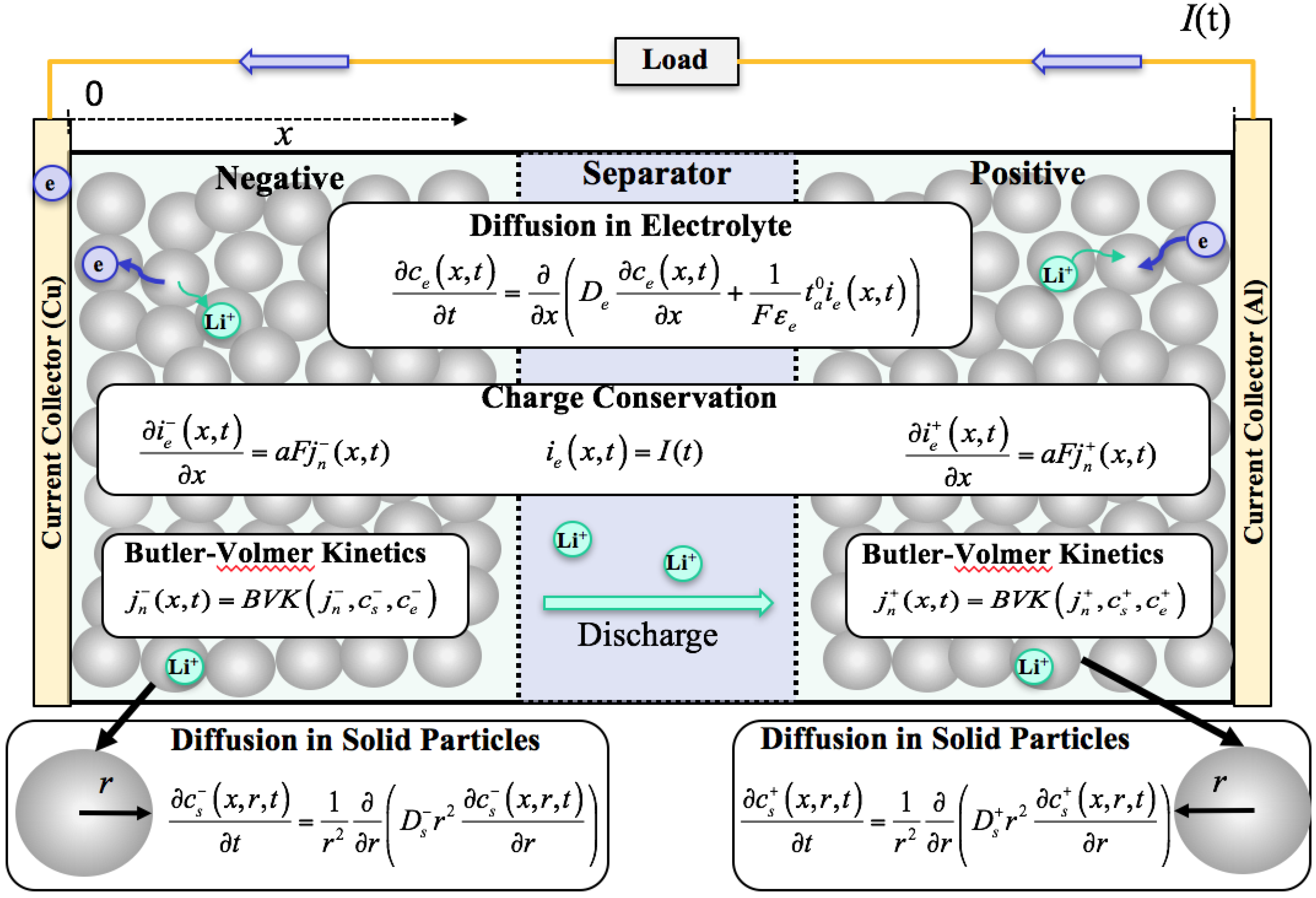
The electrochemical model consists of coupled PDEs to describe the diffusion, migration, and reaction kinetics inside the battery. Solving the electrochemical models is challenging. Doyle and Newman [14] developed an electrochemical model that takes mass transfer, diffusion, migration, and reaction kinetics into account. In the literature, this model is also called the “dualfoil” model. It is the most commonly used model for simulating the electrochemical process of the Li-ion batteries, and it has been extensively validated by experiments. In this model, the battery is divided into three domains, namely, negative electrode, separator, and positive electrode. Figure 3 shows the structure of a Li-ion battery and the governing equations of the physics process in each part of the battery. The lattice structures of the electrode active materials are modeled by small spherical particles. The transport of Li-ions in the solid electrode partials (solid phase) and electrolyte phase is modeled by diffusion equations and coupled by Butler–Volmer reaction kinetics. Using this model, the lithium concentrations and overpotentials inside the battery can be calculated. The major equations describing the physics of the battery are introduced below.

We define an x-axis starting from the negative current collector to the positive current collector, and an r-axis along the radius direction of the solid electrode particle. The transportation of the Li-ions in the solid-phase particles can be modeled by a diffusion equation as follows [14]:

$$\frac{\partial c_s\left(x,r,t\right)}{\partial t}=\frac{1}{r^2}\frac{\partial }{\partial r}\left(D_s{r}^2\frac{\partial c_s\left(x,r,t\right)}{\partial r}\right)$$

(4)

with boundary conditions and initial conditions given by:

$${\frac{\partial c_s}{\partial r}|}_{r=0}=0$$

(5)

$${\frac{\partial c_s}{\partial r}|}_{r=R_p}=-\frac{1}{D_s}{j}_n$$

(6)

$$c_s\left(x,r,0\right)=c_s^0$$

(7)

where c_s is the solid-phase concentration, j_n is the molar flux, D_s is the diffusion coefficient, and R_p is the radius of the solid-phase particle. The transportation of lithium ions in the electrolyte can be modeled as follows:

$$\frac{\partial c_e\left(x,t\right)}{\partial t}=\frac{\partial }{\partial x}\left(D_e\frac{\partial c_e\left(x,t\right)}{\partial x}+\frac{1}{F{\epsilon }_e}{t}_a^0{i}_e\left(x,t\right)\right)$$

(8)

where c_e is the lithium concentration in the electrolyte, D_e is the effective diffusion coefficient, ${\epsilon }_e$ is the volume fraction of the electrolyte, F is Faraday’s constant, and $t_a^0$ is the transference number for the anion. On the surface of solid-phase particles, an electrochemical reaction occurs when lithium ions are transferred from (to) the solid phase to (from) the electrolyte phase. The reaction flux j_n depends on the overpotential ${\eta }_s$, and this relationship can be described by the Butler-Volmer equation as

$$j_n\left(x,t\right)=\frac{i_0\left(x,t\right)}{F}\left[\exp \left(\frac{{\alpha }_{a}F}{RT}{\eta }_s\left(x,t\right)\right)-\exp \left(\frac{{\alpha }_{c}F}{RT}{\eta }_s\left(x,t\right)\right)\right]$$

(9)

where ${\alpha }_a$ and ${\alpha }_c$ are transport coefficients, and $i_0$ is the exchange current density, which is defined as

$$i_0\left(x,t\right)=r_{eff}{c}_e{\left(x,t\right)}^{{\alpha }_a}\times {\left(c_{s,max}-c_{ss}\left(x,t\right)\right)}^{{\alpha }_a}{c}_{ss}{\left(x,t\right)}^{{\alpha }_c}$$

(10)

where c_ss and c_s,max represent, respectively, the surface concentration and the maximum possible concentration in the solid particles of the electrode, and r_eff is a reaction rate constant. As shown in Equation (9), the overpotential ${\eta }_s$ determines the rate of electrochemical reactions or flux j_n and varies with time t and location x. The overpotentials are calculated by the solid-phase potential ${\mathsf{\Phi }}_s$, electrolyte potential ${\mathsf{\Phi }}_e$, open-circuit potential $U\left(c_{ss}\left(x,t\right)\right)$, and the flux j_n, as follows:

$${\eta }_s\left(x,t\right)={\mathsf{\Phi }}_s\left(x,t\right)-{\mathsf{\Phi }}_e\left(x,t\right)-U\left(c_{ss}\left(x,t\right)\right)-F{R}_f{j}_n\left(x,t\right)$$

(11)

where $F{R}_f{j}_n\left(x,t\right)$ is the potential drop due to the film resistance $R_f$ at the solid electrolyte interface. In each electrode, the flux j_n is dependent upon the divergence of current density in the electrolyte i_e,, as follows:

$$\frac{\partial i_e\left(x,t\right)}{\partial x}=aF{j}_n\left(x,t\right)$$

(12)

where a is the specific interfacial area of the particle. The i_e should be zeroes at the current collectors and should be equal to the applied current density, I, at the separator.

4. An Optimised Projection Method to Solve Solid-Phase Diffusion PDEs

In order to solve the electrochemical model, the traditional finite element and finite difference methods usually generate thousands of states, making these methods computationally intensive for real-time applications. To implement the electrochemical model in a real-time BMS where the memory and computational power are limited, an efficient numerical solution for the diffusion PDEs must be developed. In this Section, a projection-based method is developed to reduce the PDEs to a low-order DAE system. The projection-based method approximates the concentration $c_s\left(r,t\right)$ by a set of basis functions with time-varying coefficients as follows:

$$c_s\left(r,t\right)={\Phi }^{\mathrm{T}}\left(r\right)·a\left(t\right)$$

(13)

where $\Phi \left(r\right)={\left[{\varphi }_1\left(r\right),{\varphi }_2\left(r\right),\dots ,{\varphi }_N\left(r\right)\right]}^{\mathrm{T}}$ and $a\left(t\right)={\left[a_1\left(t\right),a_2\left(t\right),\dots ,a_N\left(t\right)\right]}^{\mathrm{T}}$. Once $a_i\left(t\right)$ is determined, $c_s\left(r,t\right)$ can be found accordingly. Therefore, the problem is converted into a problem of finding time-varying coefficients $a_i\left(t\right)$. First, N equations are needed, as there are N unknown $a_i\left(t\right)$. The projection-based method is used to generate the N equations based on the diffusion equation.

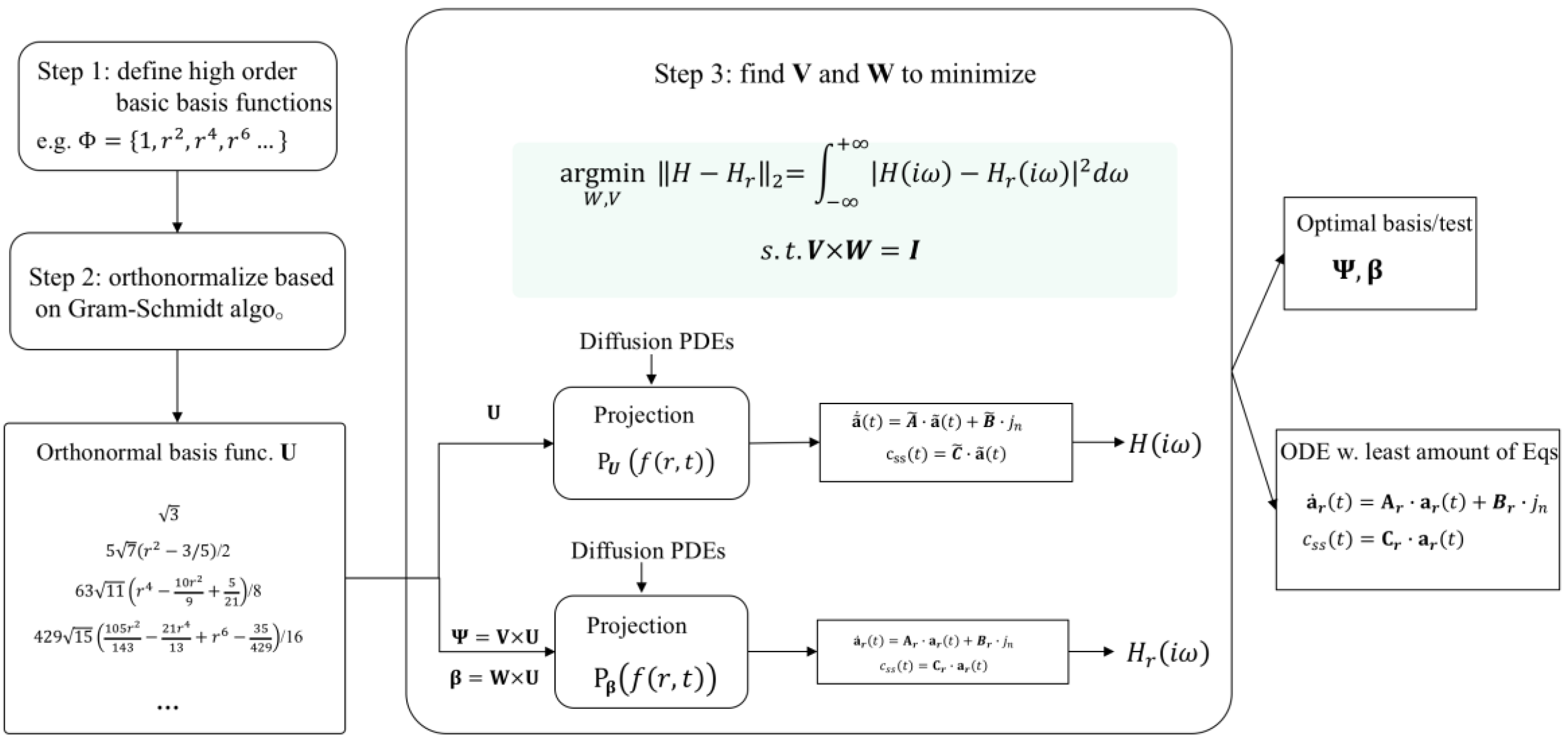
The optimized basis function is constructed in three steps: (i) definition of elementary basis functions, e.g., even-order monomials, (ii) orthonormalization of elementary basis function to ensure the numerical stability of the generated equations, and (iii) linear transformation of the orthonormal basis function. In what follows, these three steps are explained in detail:

4.1. Definition of Elementary Basis Functions

A function $\mathrm{P}:U\to U$ is called a projector if it is: (i) linear, i.e., $\mathrm{P}\left(a·f_1+b·f_2\right)=a·\mathrm{P}\left(f_1\right)+b·\mathrm{P}\left(f_2\right)$; and (ii) idempotent, i.e., ${\mathrm{P}}^2\left(f\right)=\mathrm{P}\left(f\right)$. For example, the Galerkin projector for the function $f\left(r\right)$ is given by:

$${\mathrm{P}}_{{\beta }_i}\left(f\left(r\right)\right)=\frac{{{\displaystyle \int }}_0^{R_p}{r}^{2}f\left(r\right)·{\beta }_{i}dr}{{{\displaystyle \int }}_0^{R_p}{r}^2{\beta }_i·{\beta }_{i}dr}·{\beta }_i$$

(14)

where ${\beta }_i$ is called the test function of the projector. With different test functions, the projection results are different. This property is useful for constructing different equations to calculate the time-varying coefficients in Equation (13). In this paper, we design a basis function such that the first boundary condition at the center of the particle in Equation (5) is fulfilled. An example of such a basis function is the even-order monomials (i.e., 1, r², r⁴…). By substituting the approximation to the boundary condition at the surface of the particle, we obtain the first equation as follows:

$$D_s\left({\frac{\partial {\Phi }^{\mathrm{T}}\left(x\right)}{\partial r}|}_{r=R_p}\right)·a\left(t\right)=-j_n$$

(15)

The remaining N – 1 equations are obtained by applying the projection N – 1 times to both sides of the solid-phase diffusion PDEs using different basis functions ${\beta }_i,i=1,\dots ,N-1$,

$$\begin{gathered} {\mathrm{P}}_{{\beta }_i}\left(\frac{\partial c_s\left(r,t\right)}{\partial t}\right)={\mathrm{P}}_{{\beta }_i}\left(\frac{1}{r^2}\frac{\partial }{\partial r}\left(D_s{r}^2\frac{\partial c_s\left(r,t\right)}{\partial r}\right)\right)\Rightarrow {{\displaystyle \int }}_0^{{\mathrm{R}}_p}{r}^2\frac{\partial c_s\left(r,t\right)}{\partial t}{\beta }_i\left(r\right)dr \\ ={{\displaystyle \int }}_0^{{\mathrm{R}}_p}{r}^2\left(\frac{1}{r^2}\frac{\partial }{\partial r}\left(D_s{r}^2\frac{\partial c_s\left(r,t\right)}{\partial r}\right)\right){\beta }_i\left(r\right)dr \end{gathered}$$

(16)

Integrating by parts for the right-hand side of Equation (16) and applying the boundary condition in Equations (5) and (6), we have:

$${{\displaystyle \int }}_0^{R_p}{r}^2\frac{\partial c_s\left(r,t\right)}{\partial t}{\beta }_i\left(r\right)dr=-{{\displaystyle \int }}_0^{R_p}{D}_s{r}^2\frac{\partial c_s\left(r,t\right)}{\partial r}\frac{\partial {\beta }_i\left(r\right)}{\partial r}dr-R_p{}^2{\beta }_i\left(R\right)j_n,i=1,\dots ,N-1$$

(17)

By substituting the approximation of Equation (13) into Equation (17), we obtain:

$$\begin{gathered} \left({{\displaystyle \int }}_0^{R_p}{r}^2{\Phi }^{\mathrm{T}}\left(r\right){\beta }_i\left(r\right)dr\right)·\dot{a}\left(t\right)= \\ \left(-{{\displaystyle \int }}_0^{R_p}{D}_s{r}^2\frac{\partial {\Phi }^{\mathrm{T}}\left(r\right)}{\partial r}\frac{\partial {\beta }_i\left(r\right)}{\partial r}dr\right)·a\left(t\right)+\left(-R_p{}^2{\beta }_i\left(R_p\right)\right)j_n,=1,\dots ,N-1 \end{gathered}$$

(18)

Then, the obtained differential algebraic equations are summarized as follows:

$$M·\dot{a}\left(t\right)=A·a\left(t\right)+\mathit{B}·j_n;E·a\left(t\right)=-j_n;{\mathrm{c}}_{\mathrm{ss}}\left(t\right)=C·a\left(t\right)$$

(19)

where

$$M={\left[{{\displaystyle \int }}_0^{R_p}{r}^2\mathsf{\beta }\left(r\right){\Phi }^{\mathrm{T}}\left(r\right)dr\right]}_{N-1\times N};A={\left[-{{\displaystyle \int }}_0^{R_p}{D}_s{r}^2\frac{\partial \mathsf{\beta }\left(r\right)}{\partial r}\frac{\partial {\Phi }^{\mathrm{T}}\left(r\right)}{\partial r}dr\right]}_{N-1\times N}$$

$$B={\left[-R_p{}^2\mathsf{\beta }\left(R_p\right)\right]}_{N-1\times 1};E={\left[D_s{\frac{\partial {\Phi }^{\mathrm{T}}\left(r\right)}{\partial r}|}_{r=R_p}\right]}_{1\times N};C={\left[{\Phi }^{\mathrm{T}}\left(R_p\right)\right]}_{1\times N}$$

(20)

4.2. Orthonormalization of the Basis Function

To ensure numerical stability and avoid large condition number, $\Phi$ and $\mathsf{\beta }$ have to be orthonormal basis functions, such that

$${\mathrm{Proj}}_{{\beta }_i}\left({\varphi }_j\right)=\{\begin{array}{c}1 i=j\\ 0 i\ne j\end{array}$$

(21)

and then the matrix M becomes

$$M=\left[\begin{array}{ccc}\begin{array}{cc}1& 0\\ 0& 1\end{array}& \cdots & \begin{array}{cc}0& 0\\ 0& 0\end{array}\\ ⋮& \ddots & ⋮\\ \begin{array}{cc}0& 0\end{array}& \cdots & \begin{array}{cc}1& 0\end{array}\end{array}\right]$$

(22)

Let us assume that the original elementary basis set is $\mathit{S}=\left\{{\Phi }_1,{\Phi }_2,\dots ,{\Phi }_k\right\}$. The Gram-Schmidt algorithm is used to generate a set of orthonormal basis functions $\widehat{\mathit{S}}=\left\{u_1,u_2,\dots ,u_k\right\}$ that spans the same k-dimensional space of ${ℝ}^n$ as S, and

$$\langle u_i,u_j\rangle =\{\begin{array}{c}1 i=j\\ 0 i\ne j\end{array}$$

(23)

The steps of the Gram-Schmidt algorithm are given in

Table 1. Steps of the Gram-Schmidt algorithm.

Steps	Orthogonalizing	Normalizing
Step 1:	$u_1={\phi }_1$	$u_1=\frac{u_1}{\Vert u_1\Vert }$
Step 2:	$u_2={\phi }_2-{\mathrm{Proj}}_{u_1}\left({\phi }_2\right)$	$u_2=\frac{u_2}{\Vert u_2\Vert }$
Step 3:	$u_3={\phi }_3-{\mathrm{Proj}}_{u_1}\left({\phi }_3\right)-{\mathrm{Proj}}_{u_2}\left({\phi }_3\right)$	$u_3=\frac{u_3}{\Vert u_3\Vert }$
. . .	. . .	. . .
Step k:	$u_k={\phi }_k-{\displaystyle {\displaystyle \sum }_{j=1}^{k-1}}{\mathrm{Proj}}_{u_j}\left({\phi }_k\right)$	$u_k=\frac{u_k}{\Vert u_k\Vert }$

.

4.3. Linear Transformation of the Orthonormal Basis Function

The selection of basis function has a significant effect on the approximation accuracy. In this study, we develop a method to construct an optimal basis function from a set of elementary basis functions. First, we define a set of high-order orthonormal elementary basis functions, U, formed by applying the Gram–Schmidt algorithm to even-order monomials (i.e., 1, r², r⁴…):

$$U={\left[u_1,u_2,\dots ,u_N\right]}^{\mathrm{T}}$$

(24)

We also choose the same U as the elementary test functions in the projection to satisfy the orthonormality between the basis and test functions in Equation (21). Then the M, A, B, E, and C matrices in Equation (20) become:

$$M={\left[{{\displaystyle \int }}_0^{R_p}{r}^{2}U\left(r\right)U^{\mathrm{T}}\left(r\right)dr\right]}_{N-1\times N};A={\left[-{{\displaystyle \int }}_0^{R_p}{D}_s{r}^2\frac{\partial U\left(r\right)}{\partial r}\frac{\partial U^{\mathrm{T}}\left(r\right)}{\partial r}dr\right]}_{N-1\times N}$$

$$B={\left[-R_p{}^{2}U\left(R_p\right)\right]}_{N-1\times 1};E={\left[D_s{\frac{\partial U^{\mathrm{T}}\left(r\right)}{\partial r}|}_{r=R_p}\right]}_{1\times N};C={\left[U^{\mathrm{T}}\left(R_p\right)\right]}_{1\times N}$$

(25)

The construction of the optimal basis function $\Psi$ and test function $\beta$ is accomplished by using a linear transformation given by:

$$\Psi =V\times U;=W\times U$$

(26)

where V and W are k by N matrices, and N and k are the original and reduced dimensionality with k $\ll$ N. To ensure the orthonormality of the $\Psi$ and $\mathsf{\beta }$, we must have $W^{T}V=\mathit{I}$. The concentration $c_s\left(r,t\right)$ can then be approximated by:

$$c_s\left(r,t\right)={\Psi }^{\mathrm{T}}{a}_r\left(t\right)$$

(27)

By substituting the basis and test functions in Equation (26) into Equations (19) and (20), the DAEs generated by the optimized basis and test functions are:

$$M_{\mathit{r}}·{\dot{a}}_{\mathit{r}}\left(t\right)=A_{\mathit{r}}·a_{\mathit{r}}\left(t\right)+{\mathit{B}}_{\mathit{r}}·j_n;E_{\mathit{r}}·a_{\mathit{r}}\left(t\right)=-j_n;c_{ss}\left(t\right)=C_{\mathit{r}}·a_{\mathit{r}}\left(t\right)$$

(28)

where:

$$M_{\mathit{r}}={\left[W\left({{\displaystyle \int }}_0^{R_p}{r}^{2}U\left(r\right)U^{\mathrm{T}}\left(r\right)dr\right)V^T\right]}_{k-1\times k}$$

$$A_{\mathit{r}}={\left[W\left(-{{\displaystyle \int }}_0^{R_p}{D}_s{r}^2\frac{\partial U\left(r\right)}{\partial r}\frac{\partial U^{\mathrm{T}}\left(r\right)}{\partial r}dr\right)V^T\right]}_{k-1\times k}$$

$${\mathit{B}}_{\mathit{r}}={\left[W\left(-R_p{}^{2}U\left(R_p\right)\right)\right]}_{k-1\times 1}$$

$$E_{\mathit{r}}={\left[\left(D_s{\frac{\partial U^{\mathrm{T}}\left(r\right)}{\partial r}|}_{r=R_p}\right)V^T\right]}_{1\times k};C_{\mathit{r}}={\left[\left(U^{\mathrm{T}}\left(R_p\right)\right)V^T\right]}_{1\times k}$$

(29)

Therefore, the number of DAEs is further reduced to k.

Suppose the transfer function of the DAEs based on the high-order elementary basis function is H(s), and the transfer function of the DAEs generated by the low-order optimized basis function is $H_r\left(s\right).$ The objective of the optimization is to find the transform matrices V and W to minimize the 2-norm error between H(s) and H_r(s):

$${\Vert H-H_r\Vert }_2={{\displaystyle \int }}_{-\infty }^{+\infty }{\left|H\left(i\omega \right)-H_r\left(i\omega \right)\right|}^{2}d\omega .$$

(30)

The Meier–Luenberger condition [23] provides the first-order necessary optimality condition for the optimization problem in Equation (30), which is stated as follows:

Theorem 1.

Let H(s) be the full-order system, and$H_r\left(s\right)$be the minimizer of$\Vert H\left(s\right)-H_r{\left(s\right)\Vert }_2$with simple poles${\widehat{\lambda }}_1,\dots ,{\widehat{\lambda }}_r$. Then$H(-{\widehat{\lambda }}_k)=H_r(-{\widehat{\lambda }}_k)$and$H^{\prime }(-{\widehat{\lambda }}_k)=H_r^{\prime }(-{\widehat{\lambda }}_k)$for$i=1,\dots ,r.$

To satisfy this necessary condition, we need to interpolate H(s) and its derivative at the mirror image of the poles of the reduced-order system. For linear stable ODEs, the rational Hermite interpolation provides a way to determine the W and V matrices to obtain $H_r$, and below is its definition:

Given $H\left(s\right)=C^T{\left(sI-A\right)}^{-1}B$, and r distinct points ${\mathsf{\sigma }}_1,\dots ,{\mathsf{\sigma }}_r\in ℂ$, let

$$Ran\left(V\right)=span\left\{{\left({\mathsf{\sigma }}_{1}I-A\right)}^{-1}B,\dots ,{\left({\sigma }_{r}I-A\right)}^{-1}B\right\}$$

$$Ran\left(W\right)=span\left\{{\left({\mathsf{\sigma }}_{1}I-A^{\mathit{T}}\right)}^{-1}C,\dots ,{\left({\sigma }_{r}I-A^T\right)}^{-1}C\right\}.$$

(31)

Define $A_r={\left(W^{T}V\right)}^{-1}{W}^{T}AV$;$B_r={\left(W^{T}V\right)}^{-1}{W}^{T}B$;$C_r=CV$, then $H_r\left(s\right)=C_r^T{\left(s{I}_r-A_r\right)}^{-1}{B}_r$ is a rational Hermite interpolate to $H\left(s\right)$ at ${\mathsf{\sigma }}_1,\dots ,{\mathsf{\sigma }}_r$, and $H\left({\sigma }_i\right)=H_r\left({\sigma }_i\right)$ and $H^{\prime }\left({\sigma }_i\right)=H_r^{\prime }\left({\sigma }_i\right)$, for $i=1,\dots ,r$. The rational Hermite interpolate can be directly used to find V and W to construct $H_r$, if the poles of $H_r$ are known. However, this information is not known as a prior. In this case, the iterative rational Krylov algorithm (IRKA) can be used to iteratively correct the interpolation points until the local minimum is found [24]. The steps of IRKA are defined below:

• Make an initial selection of ${\sigma }_i$ for $i=1,\dots ,r$ that is closed under conjugation.
• Choose V and W such that:

  $$\begin{gathered} Ran\left(V\right)=span\{{\left({\sigma }_{1}I-A\right)}^{-1}B,\dots ,{\left({\sigma }_{r}I-A\right)}^{-1}B\}; \\ Ran\left(W\right)=span\{{\left({\sigma }_{1}I-A\right)}^{-1}C,\dots ,{\left({\sigma }_{r}I-A\right)}^{-1}C\};\mathrm{where}{W}^{T}V=I \end{gathered}$$
• While relative change in $\left\{{\sigma }_i\right\}>tol$
  • $A_r=W^{T}AV$
  • Assign ${\sigma }_i\leftarrow -{\lambda }_i\left(A_r\right)$ for i = 1,…,r
  • Update V and W, such that

    $$\begin{array}{l}Ran\left(V\right)=span\{{\left({\sigma }_{1}I-A\right)}^{-1}B,\dots ,{\left({\sigma }_{r}I-A\right)}^{-1}B\};\\ Ran\left(W\right)=span\{{\left({\sigma }_{1}I-A\right)}^{-1}C,\dots ,{\left({\sigma }_{r}I-A\right)}^{-1}C\};\mathrm{where}{W}^{T}V=I\end{array}$$
• $A_r=W^{T}AV$, $=W^{T}B$, $C_r=CV$

The IRKA was developed originally for asymptotically stable systems, i.e., all of the eigenvalues of the pencil (A, I) must be in the left half of the complex plane. However, our system is unstable, therefore the IRKA is not directly applicable. To solve this problem, we first convert the DAEs into ODEs. Let us assume that R = [M; E]. If R is invertible, then the DAEs in Equation (19) can be transformed to ODEs [15]. Let:

$$z=M·a;{\mathit{R}}^{-1}=\left[\begin{array}{cc}{\mathit{Q}}_1& {\mathit{Q}}_2\end{array}\right]$$

(32)

where ${\mathit{Q}}_1\in {ℝ}^{N-1\times N}$ and ${\mathit{Q}}_2\in {ℝ}^{N-1\times 1}$, then we have

$$a={\left[\begin{array}{c}M\\ E\end{array}\right]}^{-1}\left[\begin{array}{c}z\\ -j_n\end{array}\right]=\left[\begin{array}{cc}{\mathit{Q}}_1& {\mathit{Q}}_2\end{array}\right]\left[\begin{array}{c}z\\ -j_n\end{array}\right]={\mathit{Q}}_{1}z-{\mathit{Q}}_2{j}_n$$

(33)

By substituting Equation (33) into Equation (19), we obtain the ODEs:

$$\dot{z}=A\left({\mathit{Q}}_{1}z-{\mathit{Q}}_2{j}_n\right)+B{j}_n=A{\mathit{Q}}_{1}z+\left(B-A{\mathit{Q}}_2\right)j_n$$

$${\mathrm{c}}_{\mathrm{ss}}\left(t\right)=C\left({\mathit{Q}}_{1}z-{\mathit{Q}}_2{j}_n\right)=C{\mathit{Q}}_{1}z-C{\mathit{Q}}_2{j}_n$$

(34)

Since $\left[u_1,u_2,\dots ,u_N\right]$ are orthonormal, [M; E] is:

$$\left[\begin{array}{c}M\\ E\end{array}\right]=\left[\begin{array}{cccccc}1& 0& 0& \cdots & 0& 0\\ 0& 1& 0& \cdots & 0& 0\\ 0& 0& 1& \cdots & 0& 0\\ ⋮& ⋮& ⋮& \ddots & ⋮& ⋮\\ 0& 0& 0& \cdots & 1& 0\\ 0& D_s{u}_2^{\prime }& D_s{u}_3^{\prime }& \cdots & D_s{u}_{N-1}^{\prime }& D_s{u}_N^{\prime }\end{array}\right]$$

(35)

It is straightforward to prove that the inverse of Equation (35) is:

$${\left[\begin{array}{c}M\\ E\end{array}\right]}^{-1}=\left[\begin{array}{cccccc}1& 0& 0& \cdots & 0& 0\\ 0& 1& 0& \cdots & 0& 0\\ 0& 0& 1& \cdots & 0& 0\\ ⋮& ⋮& ⋮& \ddots & ⋮& ⋮\\ 0& 0& 0& \cdots & 1& 0\\ 0& -\frac{u_2^{\prime }}{u_N^{\prime }}& -\frac{u_3^{\prime }}{u_N^{\prime }}& \cdots & -\frac{u_{N-1}^{\prime }}{u_N^{\prime }}& \frac{1}{D_s{u}_N^{\prime }}\end{array}\right].$$

(36)

Because u₁ = 1, the first column and first row of A in Equation (20) are zeros. Therefore, the first row and first column of $A{\mathit{Q}}_1$ are zeros, and the ODEs are obtained as follows:

$$\left[\begin{array}{c}{\dot{\mathrm{z}}}_1\left(t\right)\\ {\dot{Z}}_{\mathbf{2}}\left(t\right)\end{array}\right]=\left[\begin{array}{cc}0& \mathbf{0}\\ \mathbf{0}& {\overline{A}}_{\mathbf{2}}\end{array}\right]z\left(t\right)+\left[\begin{array}{c}{\overline{\mathrm{B}}}_1\\ {\overline{B}}_{\mathbf{2}}\end{array}\right]·j_n\left(t\right)$$

$$c_{ss}\left(t\right)=\left[\begin{array}{cc}{\overline{\mathrm{C}}}_1& {\overline{C}}_{\mathbf{2}}\end{array}\right]·{\left[{\mathrm{z}}_1\left(t\right),Z_{\mathbf{2}}\left(t\right)\right]}^{\mathrm{T}}+\overline{\mathrm{D}}·j_n\left(t\right)$$

(37)

where $Z_{\mathbf{2}}={\left[{\mathrm{z}}_2,{\mathrm{z}}_3,\dots ,{\mathrm{z}}_N\right]}^{\mathrm{T}}$. Then, we decompose the system into a stable part and an unstable part, and the IRKA is only applied to the stable part of the system. Therefore,

$$\{\begin{array}{c}{\dot{\mathrm{z}}}_1\left(t\right)={\overline{\mathrm{B}}}_1·j_n\left(t\right)\\ {\dot{Z}}_{\mathbf{2}}\left(t\right)={\overline{A}}_{\mathbf{2}}·Z_{\mathbf{2}}\left(t\right)+{\overline{B}}_{\mathbf{2}}·j_n\left(t\right)\end{array}$$

$$y\left(t\right)={\overline{\mathrm{C}}}_1·{\mathrm{z}}_1\left(t\right)+{\overline{C}}_{\mathbf{2}}·Z_{\mathbf{2}}\left(t\right)+\overline{\mathrm{D}}·j_n\left(t\right)$$

(38)

The transfer function of Equation (38) is:

$$H\left(s\right)={\overline{\mathrm{C}}}_1{s}^{-1}{\overline{\mathrm{B}}}_1+\underset{\mathrm{to}\mathrm{be}\mathrm{reduced}\mathrm{by}\mathrm{IRKA}}{\underbrace{{\overline{C}}_{\mathbf{2}}{(s·I-{\overline{A}}_{\mathbf{2}})}^{-1}{\overline{B}}_{\mathbf{2}}}}+\overline{\mathrm{D}}$$

(39)

In the IRKA, only ${\overline{C}}_2{\left(sI-{\overline{A}}_{\mathbf{2}}\right)}^{-1}{\overline{B}}_2$ will be reduced, and the remaining part stays the same. Supposing that the transformation matrices generated in IRKA are V₂ and W₂, then the transformation matrices V and W are:

$$V=\left[\begin{array}{ccc}1& \mathbf{0}& 0\\ \mathbf{0}& V_{\mathbf{2}}& \mathbf{0}\\ 0& \mathbf{0}& 1\end{array}\right], W=\left[\begin{array}{ccc}1& \mathbf{0}& 0\\ \mathbf{0}& W_{\mathbf{2}}& \mathbf{0}\\ 0& \mathbf{0}& 1\end{array}\right].$$

(40)

Then we can use Equation (26) to obtain the optimized basis function. Figure 4 summarizes the steps of the optimal projection method developed in this paper for solving diffusion PDEs.

5. Moving-Window Filter for Electrochemical SOC Estimation

Conventional state filtering methods such as the Kalman filter are sequential estimation algorithms which utilize the measurements at a single time point to provide the state estimation. Figure 5a shows a schematic plot for conventional sequential state filters. As mentioned earlier, the conventional approaches are computationally efficient, however, they may converge very slowly and may not be robust to outliers in the measurement. Therefore, this Section develops a new state filter algorithm based on the moving window to ensure the fast convergence of the proposed electrochemical SOC estimation model. In this method, more data points are used for estimation of the battery SOC. As shown in Figure 5b, a moving window of N data points (from T–N + 1 to T) is used to provide state estimation at T–N + 1. The estimation accuracy and robustness should be improved as more data points are involved in the estimations. The key question is how to calculate filter gain in this method.

The filter gain of the moving-window filter (MWF) is derived based on the maximum likelihood theory. The derivation of the filter gain assumes: (1) the measurement noise and process noise are Gaussian distributed with zero mean; (2) the system equations are continuously differentiable. Let us consider a maximum likelihood estimation problem:

$$\underset{x_{T-N+1}}{\mathrm{argm}max}P(x_{T-N+1}|y_0,y_1,\dots ,y_T)$$

(41)

Based on Bayes’ theorem [25], we have the following:

$$\underset{x_{T-N+1}}{\mathrm{argm}max}\frac{P\left(y_0,y_1,\dots ,y_T|x_{T-N+1}\right)P\left(x_{T-N+1}\right)}{P\left(y_0,y_1,\dots ,y_T\right)}$$

$$=\underset{x_{T-N+1}}{\mathrm{argm}max}\frac{P\left(y_0,y_1,\dots ,y_{T-N}|x_{T-N+1}\right){{\displaystyle \prod }}_{k=T-N+1}^{T}P\left(y_k|x_k\right)P\left(x_{T-N+1}\right)}{P\left(y_0,y_1,\dots ,y_T\right)}$$

$$\underset{x_{T-N+1}}{=\mathrm{argm}max}\frac{P\left(x_{T-N+1}|y_0,y_1,\dots ,y_{T-N}\right)P\left(y_0,y_1,\dots ,y_{T-N}\right){{\displaystyle \prod }}_{k=T-N+1}^{T}P(y_k|x_k)P\left(x_{T-N+1}\right)}{P\left(y_0,y_1,\dots ,y_T\right)P\left(x_{T-N+1}\right)}$$

$$=\underset{x_{T-N+1}}{\mathrm{argm}max}P\left(x_{T-N+1}|y_0,y_1,\dots ,y_{T-N}\right) {{\displaystyle \prod }}_{k=T-N+1}^{T}P(y_k|x_k)$$

(42)

Equation (42) is equivalent to a quadratic estimation problem as follows:

$$\underset{x_{T-N+1}}{\arg min}\Phi \left(x_{T-N+1}\right)= {\left(\mathit{y}-\mathit{H}\left({\widehat{x}}_{T-N+1}\right)\right)}^T{\mathit{R}}^{-1}\left(\mathit{y}-\mathit{H}\left({\widehat{x}}_{T-N+1}\right)\right)$$

$$+{\left(x_{T-N+1}-{\widehat{x}}_{T-N+1}\right)}^T{{\displaystyle \prod }}_{T-N+1}^{-1}\left(x_{T-N+1}-{\widehat{x}}_{T-N+1}\right)$$

(43)

In Equation (43), ${{\displaystyle \prod }}_{\mathit{T}-\mathit{N}+\mathbf{1}}{\mathit{C}}^{\mathbf{T}}{({\mathit{R}}^{\mathbf{T}}+{\mathit{C}}^{\mathbf{T}}{{\displaystyle \prod }}_{\mathit{T}-\mathit{N}+\mathbf{1}}\mathit{C})}^{-\mathbf{1}}$ is the gain of the filter. The gain has a similar structure as the Kalman filter, however the definition of the matrices in the gain is different from the Kalman filter. Based on first-order optimality given by:

$$\frac{\partial \mathsf{\Phi }\left({\mathrm{x}}_{T-N+1}\right)}{\partial {\mathrm{x}}_{T-N+1}}=0$$

(44)

we have:

$$x_{T-N+1}={\widehat{x}}_{T-N+1}+{{\displaystyle \prod }}_{T-N+1}{C}^{\mathrm{T}}{(R^{\mathrm{T}}+C^{\mathrm{T}}{{\displaystyle \prod }}_{T-N+1}C)}^{-1}(\mathbf{y}-\mathit{H}({\widehat{x}}_{T-N+1}\left)\right)$$

(45)

where:

$$\mathit{y}={[{\mathrm{y}}_{T-N+1},{\mathrm{y}}_1,\dots ,{\mathrm{y}}_T]}^{\mathrm{T}}$$

(46)

$$\mathit{H}\left(\mathit{x}\right)= {\left[\begin{array}{c}h\left(x\right)\\ h(f\left(x\right)\\ h(f\left(f\left(x\right)\right)\\ \dots \\ h(f\left(f\left(\dots f\left(x\right)\right)\right)\end{array}\right]}_{N\times 1}$$

(47)

$$C=\frac{\partial \mathit{H}\left(x_{T-N+1}\right)}{\partial x_{T-N+1}},$$

(48)

$${\widehat{x}}_{T-N+1} :mean of P\left(x_{T-N+1}|y_0,y_1,\dots ,y_{T-N}\right)$$

(49)

$${{\displaystyle \prod }}_{\mathit{T}-\mathit{N}+\mathbf{1}}: cov. of P\left(x_{T-N+1}|y_0,y_1,\dots ,y_{T-N}\right)$$

(50)

The implementation of the MWF algorithm for SOC estimation using the proposed electrochemical model is illustrated in Figure 6.

6. Case Studies

In this study, the optimal basis function is constructed from $\Phi \left(x\right)={\left[1,r^2,r^4,\dots ,r^{20}\right]}^{\mathrm{T}}$. First, the Gram–Schmidt algorithm is applied to $\Phi$ to obtain the orthonormal elementary basis and test functions, $U={\left[u_1,u_2,\dots ,u_N\right]}^{\mathrm{T}}$. The model parameters, including the diffusion coefficient D_s = 3.9 × 10^–10 cm²/s and particle radius R_p = 12.5 × 10^–4 cm, were obtained from [26]. These model parameters have shown good agreement with experimental data of Li_xC₆\Li_yMn₂O₄ cells in [9].

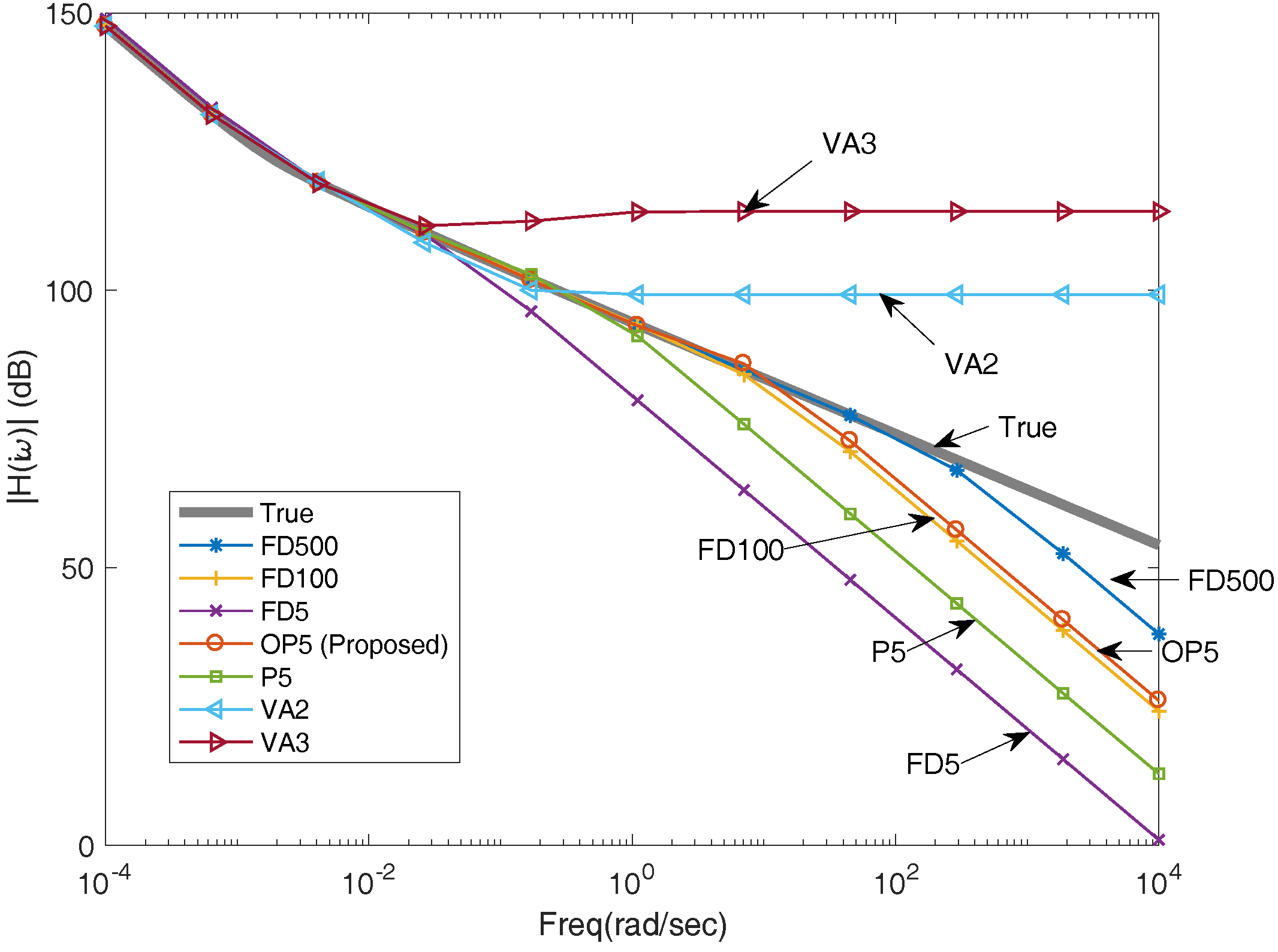
To compare the developed approach with available methods, the frequency responses of different methods are calculated, including finite difference (FD), volume averaging (VA), projection with even-order monomials (P), and our proposed method, i.e., projection with optimized basis functions (OP). The actual transfer function of the diffusion equation is given by [27]:

$$H_T\left(s\right)=\frac{R_p}{D_s}\frac{\tanh \left(R_p\sqrt{s/D_s}\right)}{\left(\tanh \left(R_p\sqrt{s/D_s}\right)-R_p\sqrt{s/D_s}\right)}$$

(51)

Figure 7 shows the frequency responses of different methods compared with the true transfer function. At low frequency (e.g., <10^–2 rad/s), all methods well match the true transfer function. As the frequency increases, we see different performances for different methods. Overall, the FD method with 500 nodes (FD500) shows the best performance. However, it requires solving 500 equations, which is not feasible for real-time applications. Our proposed projection method with optimized basis functions (OP) shows the best balance between accuracy and computational burden among those methods.

As can be seen in Figure 7, OP5 outperforms all other methods except for FD500. For example, OP5 is better than FD100 in the high-frequency domain, while it only requires solving about 20 times fewer equations compared to FD100. As expected, OP5 also outperforms VA and the projection with un-optimized basis functions (P5). The VA method developed in [17] performs well in the low-frequency domain but generates large errors in the high-frequency domain. In addition, VA3 with 3 basis functions is worse than VA2 with 2 basis functions, although more basis functions are used in VA3 because the system equations generated by VA become unstable when using high-order monomials.

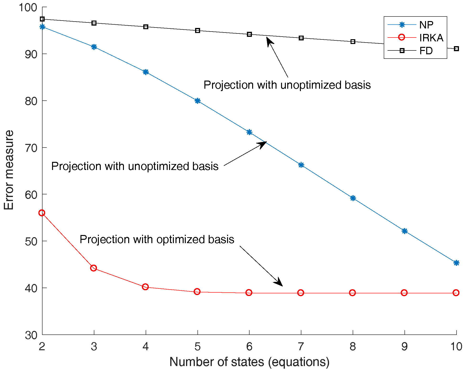
More simulations were conducted to illustrate how the error changes with the number of states (or the convergence rate). Based on this investigation, we can determine how many states are really necessary. Figure 8 shows a convergence rate comparison of the different methods. The relative error is calculated by the following equation in the frequency domain:

$$Error={{\displaystyle \int }}_0^w\frac{\Vert H\left(i\omega \right)-H_T{\left(i\omega \right)\Vert }_2}{\Vert H_T{\left(i\omega \right)\Vert }_2}d\omega$$

(52)

The OP shows an exponential convergence rate, while the finite difference and the projection with original un-optimized basis present a linear convergence rate. The advantage of the proposed OP method is obvious. From Figure 8, the accuracy of the proposed OP with three states is similar to that of the unoptimized basis with 10 states and is two times better than FD with 10 states. With five states, the OP is almost converged, and there is no need to add more states.

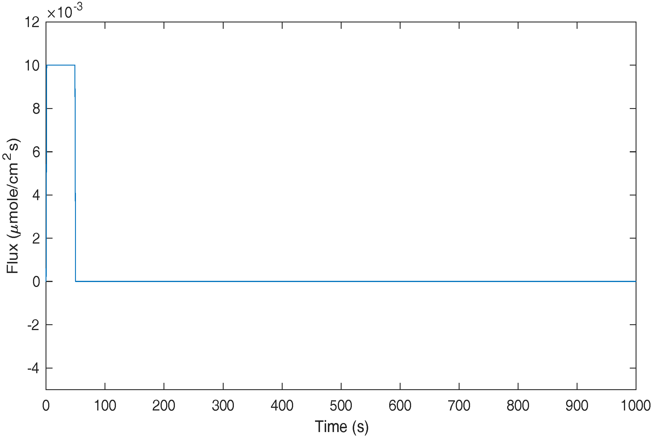
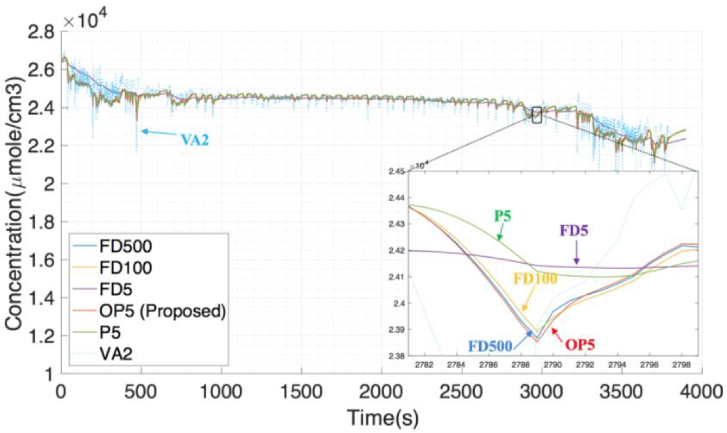
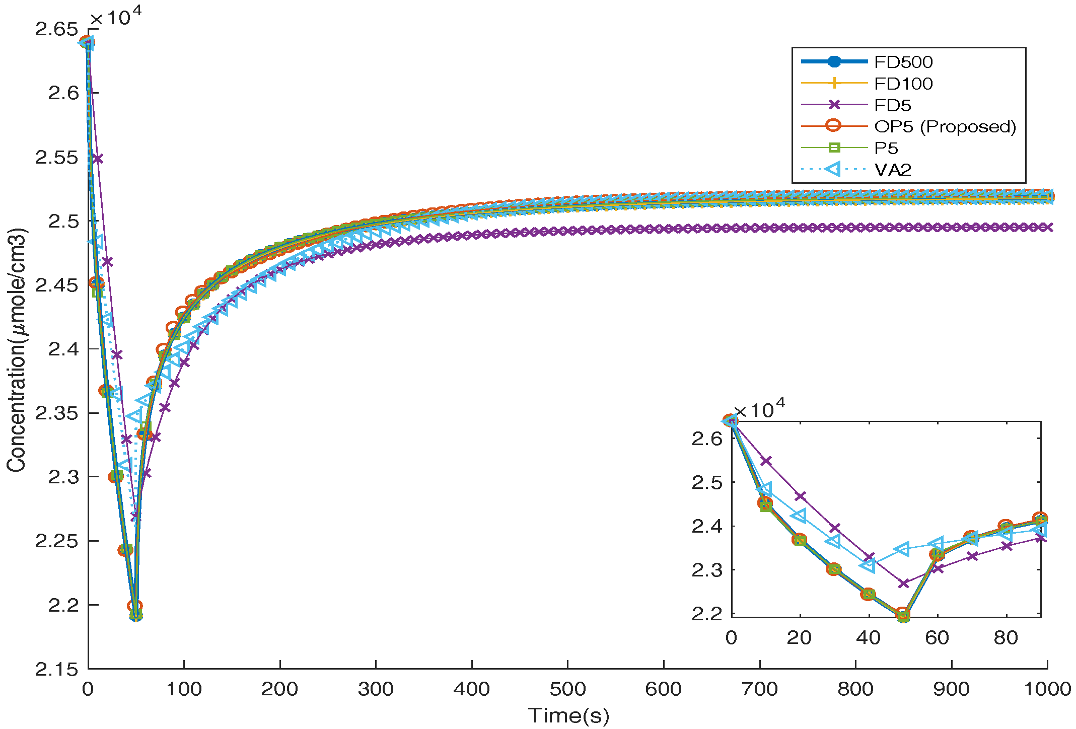
To compare the performance in the time domain, three simulations were conducted with the time-varying flux j_n(t). The first case was a 50 s discharge step followed by a 950 s rest step as shown in Figure 9. This is to evaluate the algorithms’ performance in slow dynamics and steady-state simulations. The benchmarking result is obtained by using a FD method with 500 nodes, which is an accurate solution due to the high number of nodes used. The time-domain outputs using different methods are calculated and plotted in Figure 10. In the 50 s discharge step, the results of FD100, P5, and OP5 are on top of that of FD500, meaning they are accurate for slow dynamics. VA2 and FD5 are less accurate as they show obvious discrepancy from FD500 in the concentration estimation. In the rest step, after 950 s rest, the system dynamics should set down and converge to steady state. In this step, most algorithms, including FD500, FD100, P5, OP5, and VA2, are converged to the same steady-state solution. However, FD5 shows a different steady-state solution, which can cause issues in actual applications, for example, errors in SOC estimation.

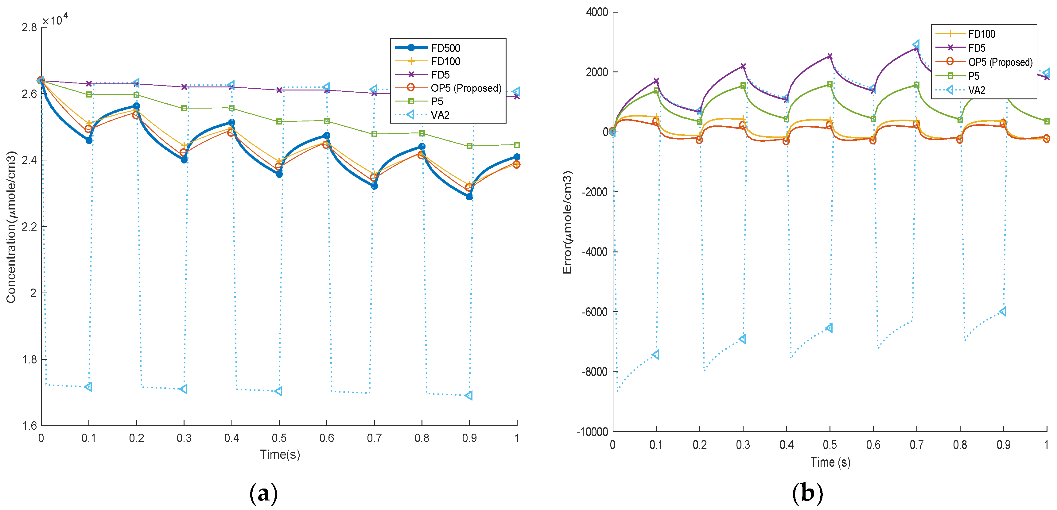
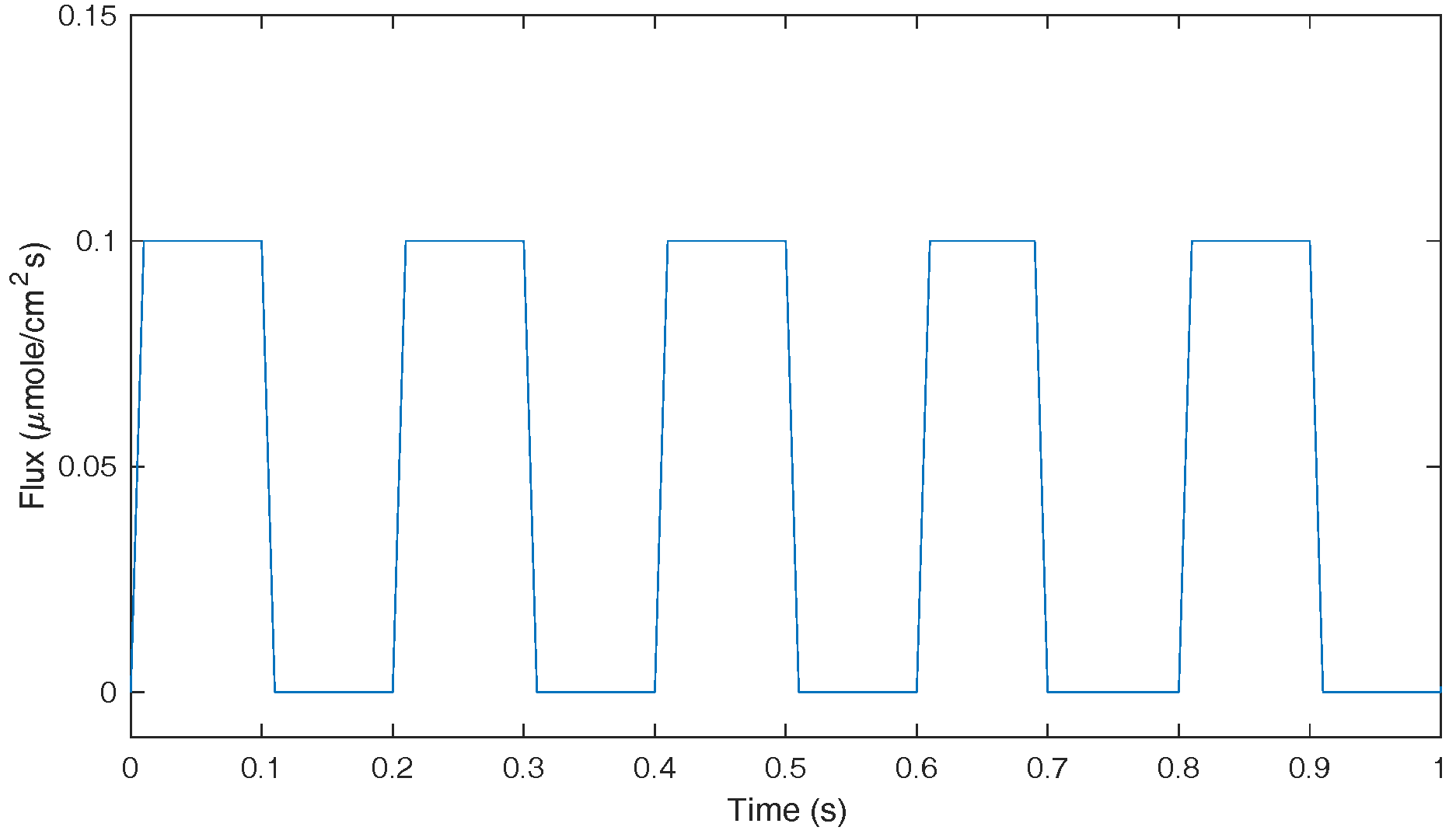
The second simulation uses a pulse series with frequency of 5 Hz and duration of 100 s, which is to evaluate the algorithms’ accuracy in the simulation for fast dynamics. The waveform of the pulses is shown in Figure 11 (only the first second of data is plotted in order to show the data clearly).

The time-domain results and the errors comparing to baseline (FD500) are illustrated in Figure 12.

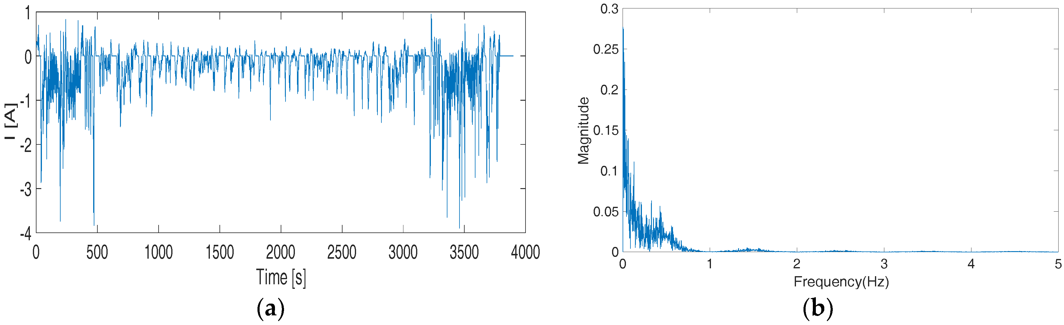
Like the frequency domain results presented in Figure 7, in the high-frequency simulations, our proposed OP5 shows obvious advantages comparing to P5, VA2, and FD5 as it better matches the results of FD500. The VA2 and FD5 perform rather poorly and show large swings from the baseline. The third case is based on federal driving schedule (FDS) to simulate the actual loading condition of an EV battery. The time-domain current waveform and its Fourier transform are shown in Figure 13. As can be seen, the main frequency components of FDS are less than 2 Hz. In Figure 7, the transfer function of FD500 overlaps with the true transfer function for frequencies <2 Hz. Hence, here we can still use FD500 as a baseline for the comparison.

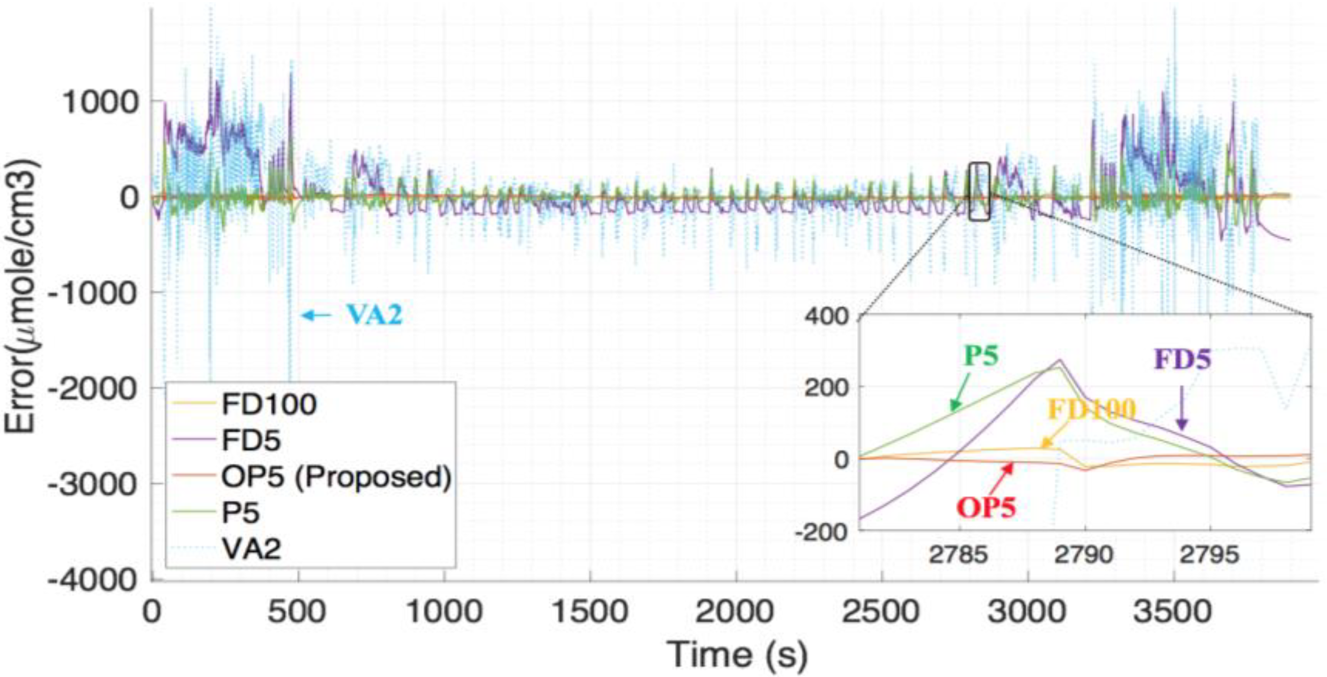
Figure 14 shows the simulation results of FDS based on different algorithms, and Figure 15 shows the simulation errors. Similar to the previous case, FD100 and OP5 are still the best among all methods.

Table 2. Comparison of algorithm performance for diffusion PDE calculation.

Algorithm	Simulation Time (s)	# Equations	RMS Error (µmol/cm3)	Memory (Byte)
FD100	12	100	18	81,680
FD5	0.44	5	271	288
OP5 (PROPOSED)	0.42	5	14	288
P10	1.21	10	16	1768
P5	0.43	5	92	488
VA2	0.41	2	382	88

summarizes the comparison of the root mean square error (RMSE), computational time, and memory requirements (for the equation storage) of difference algorithms in the simulation of the FDS. As shown, OP5 has the least RMS error among all algorithms. OP5 reduces the computational time and memory by over 20 and 200 times, respectively, compared to FD100 and is more accurate. With the same number of states, the proposed OP5 is also much better than the conventional P5 method, where the RMS error is reduced from 92 to 14.

The simulations above demonstrate that FD100, P5, and the proposed OP5 performs similarly for low-frequency inputs in terms of accuracy. For high-frequency inputs, our developed method is superior to FD100 and P5. For applications where the current profile is stationary (e.g., constant current discharge), either FD100, P5, or OP5 should provide good performance. For dynamical applications, for instance, EVs, where the current consists of various transients due to starting, braking, and accelerating, the proposed OP5 method is the best among all the methods investigated in terms of accuracy and computational efficiency.

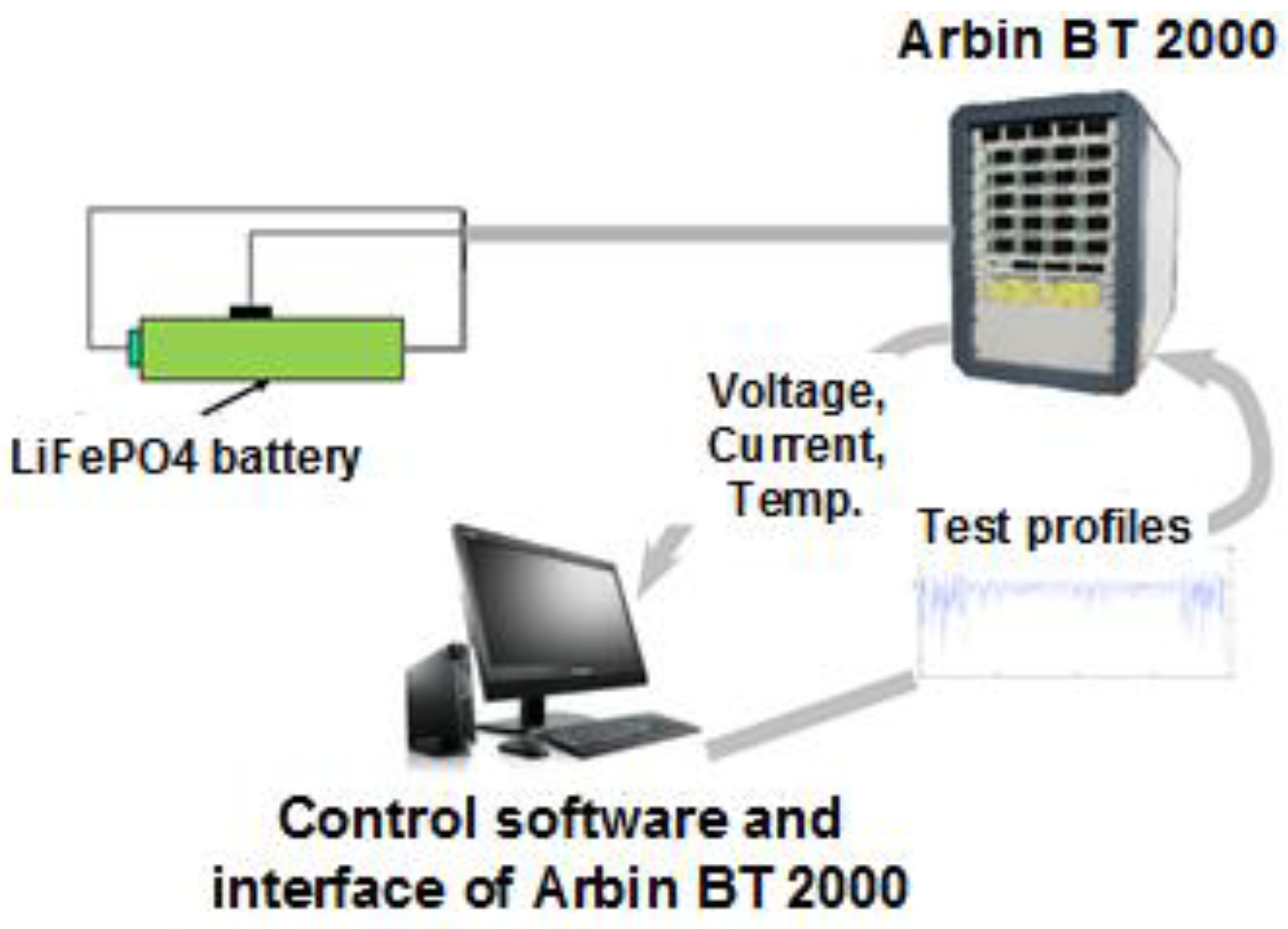
To validate the proposed MWF approach, experiments were conducted to collect battery data. Figure 16 shows the experimental setup. Five LiFePO₄ batteries were tested in this research. Arbin BT 2000 was used to control the battery charging discharge, and the voltage, current, and temperature data of the battery were collected.

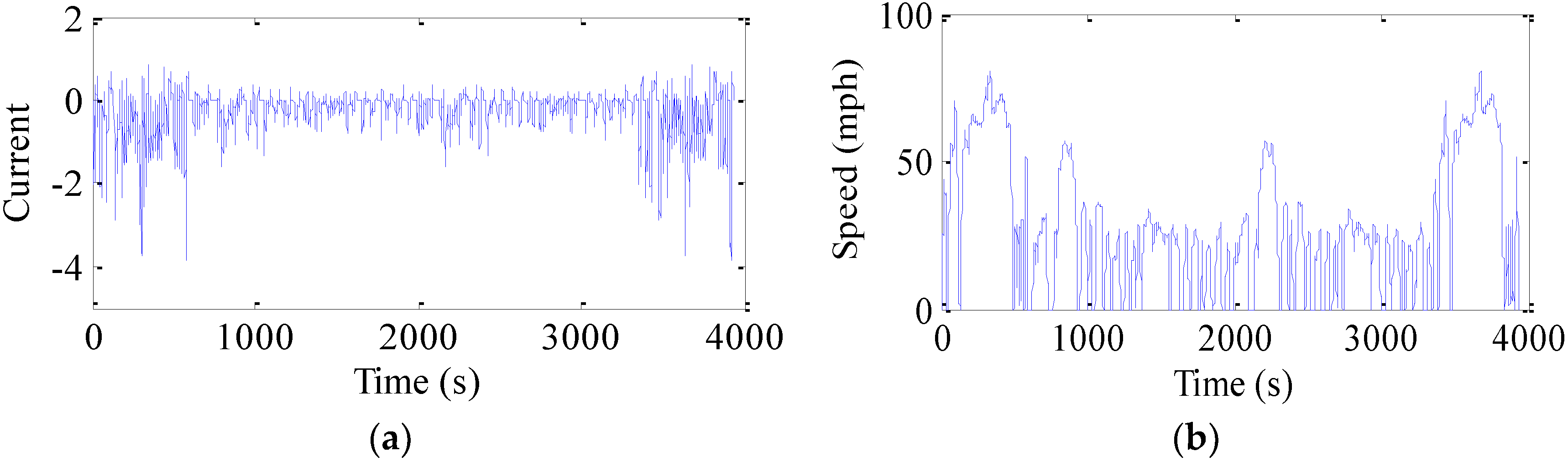
Figure 17 shows the current profile used in the test, which is converted from the speed profile of federal driving schedule (FDS) based on an EV model. This is in order to simulate what the battery can experience under the actual driving conditions.

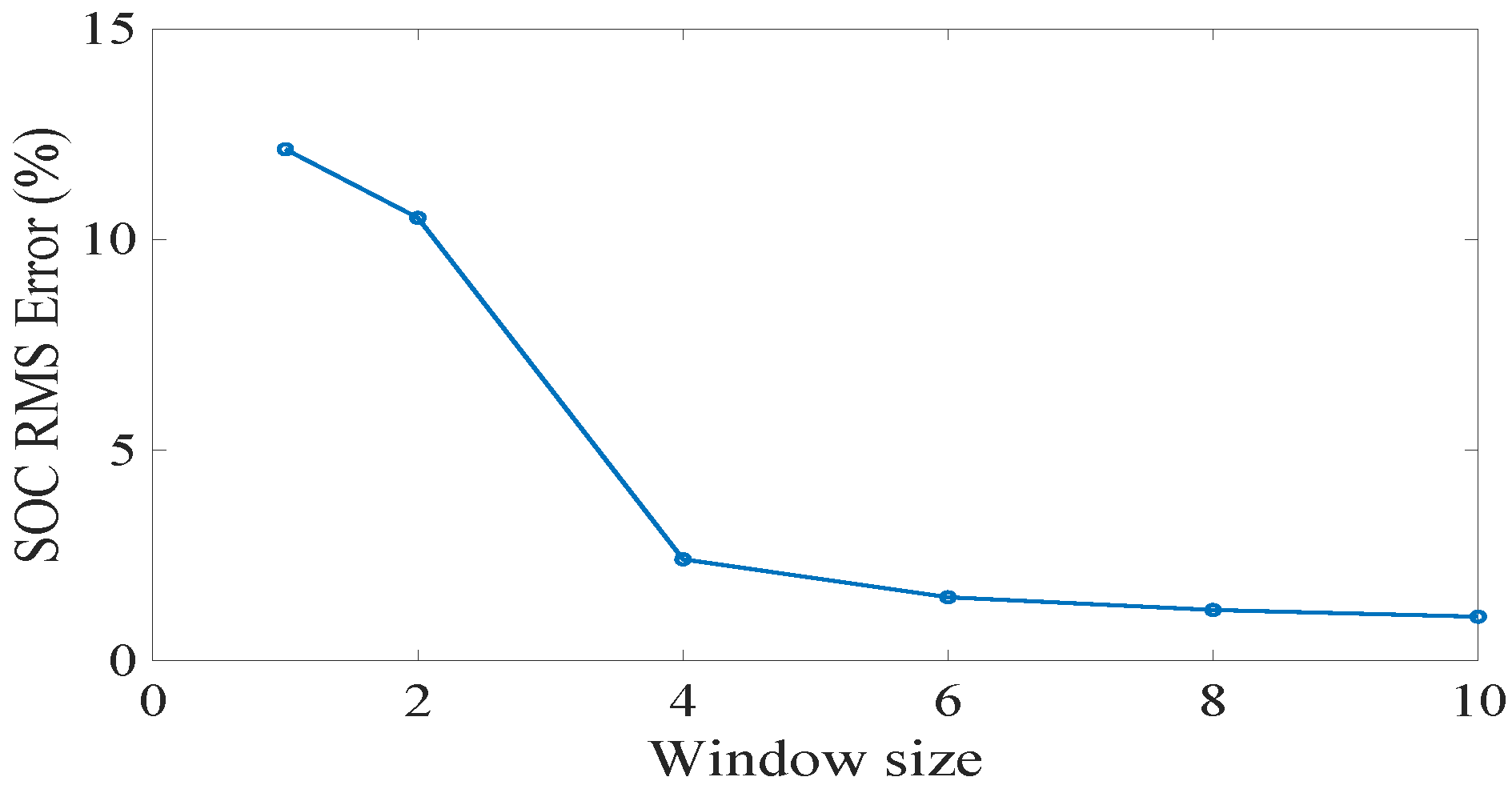
The collected data is used to test the performance of the MWF with the electrochemical model. The electrochemical model parameters were obtained from [28]. First, we examined the effects of the window size on the SOC accuracy. Figure 18 shows the results. We can see that the SOC estimation error reduces with the increasing of window size, especially when the window size increases from 2 to 4. After 4, there is not much improvement. Hence, in the next paragraphs, we will use a window size of 4 for the state estimation and compare the results with unscented Kalman filter (UKF).

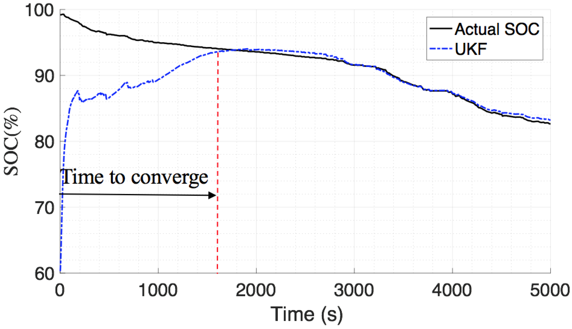
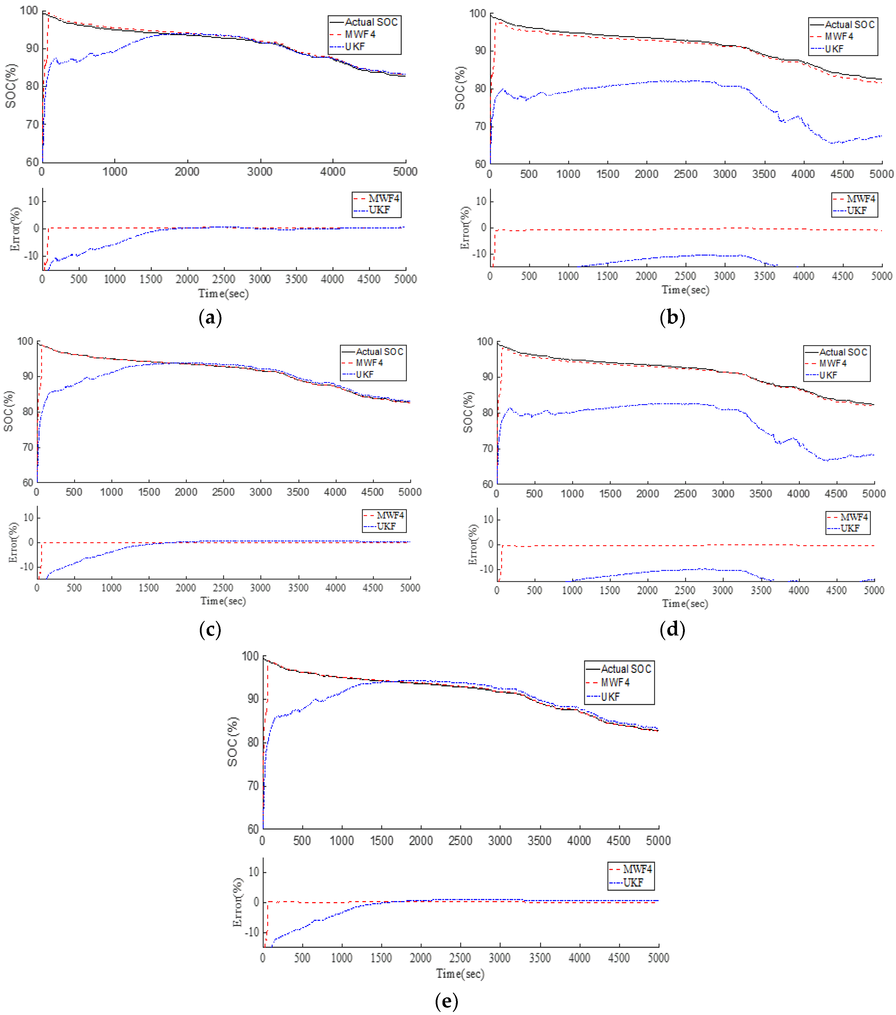
Figure 19 shows the comparison results of Cell #1 to Cell #5. The black line is the actual SOC, which was obtained by Coulomb counting because we know the initial condition and the sensor is accurate in the lab. The red line is the MWF, which converges to the true value in less than 2 min. The UKF result is represented by the blue line. It takes about 30 min for the UKF to converge. Therefore, the MWF outperforms the UKF and shows consistent improvements over the UKF.

Table 3. Summary of SOC estimation results based on electrochemical model and MWF.

Cell ID	Root Mean Square Error (first 10 min)
	UKF	MWF
Cell 1	12.1%	2.4%
Cell 2	19.7%	2.5%
Cell 3	12.4%	1.5%
Cell 4	18.1%	2.1%
Cell 5	12.1%	1.6%

summarizes the results of all 5 cells. For convergence analysis, only the first few minutes are important as we want to see which filter converges faster. Therefore, in Table 3, only the first 10 min of errors were estimated. We can see the MWF’s improvement over the UKF is significant as the SOC error decreases from >10% to 3%. The computationally efficient electrochemical model is used here with state filters for SOC estimation. The MWF not only converges fast, but also demonstrates good capability to handle unit-to-unit variations, because here the model parameters are learned from Cell #1 and then the same parameter set is applied to different cells.

7. Contributions and Suggestions for Future Research

In this paper, an electrochemical model was presented for the state-of-charge (SOC) estimation of lithium-ion batteries involving their internal physical and chemical properties such as lithium concentrations. To reduce the computational complexity of solid-phase diffusion partial differential equations (PDEs)—which is the major bottleneck for the application of any electrochemical model in a real-time battery management system—a projection-based method with optimized orthonormal basis functions was developed. The optimized basis function was constructed by linear transforming a set of orthonormal elementary basis functions. The linear transformation matrices were found by using the iterative rational Krylov algorithm. Simulation studies were conducted to compare the performance of the developed method with other commonly used algorithms, including finite difference, volume average, and the projection method with conventional basis functions. The results showed that the developed method with optimized basis functions was the best in terms of accuracy and computational complexity among all the investigated algorithms. Particularly, in the simulation of high-frequency inputs, which is common for EVs, the developed method reduced the root mean square error by more than five times compared to the conventional basis functions. In addition, compared with the finite difference method, the developed method can cut the computational time and memory requirement by over 20 times and 200 times, respectively, without losing any accuracy. The developed method can be applied in the future to solve electrolyte diffusion PDEs, and with proper modification, it can be extended to solve 2-D or 3-D diffusion PDEs by adding basis functions in other dimensions.

This study also presented a moving-window filter (MWF) algorithm which converged faster than conventional state filtering methods such as Kalman filter. The filter gain was derived based on maximum likelihood theory. The MWF was implemented with the computationally efficient electrochemical model developed in the first part, and it was validated using experimental data based on the federal driving schedule. It showed that the MWF reduced the convergence time from 30 min to less than 2 min compared with unscented Kalman filter for the SOC estimation.

Future research can focus on how to take the battery aging into account for SOC estimation. For electrochemical models, it means that the model parameters have to be updated with aging, for example, the cyclable lithium will diminish and the film resistance will grow with aging. In addition, to avoid out-of-range estimations, constraints must be implemented for the optimization, as a result, iterative optimizations may be necessary. How to reduce the computational complexity of the optimization and how to ensure the convergence of the optimization for on-line parameter estimation can be topics for future research.