Abstract
A numerical model is presented for the estimation of Wave Energy Converter (WEC) performance in variable bathymetry regions, taking into account the interaction of the floating units with the bottom topography. The proposed method is based on a coupled-mode model for the propagation of the water waves over the general bottom topography, in combination with a Boundary Element Method for the treatment of the diffraction/radiation problems and the evaluation of the flow details on the local scale of the energy absorbers. An important feature of the present method is that it is free of mild bottom slope assumptions and restrictions and it is able to resolve the 3D wave field all over the water column, in variable bathymetry regions including the interactions of floating bodies of general shape. Numerical results are presented concerning the wave field and the power output of a single device in inhomogeneous environment, focusing on the effect of the shape of the floater. Extensions of the method to treat the WEC arrays in variable bathymetry regions are also presented and discussed.
1. Introduction
Interaction of the free-surface gravity waves with floating bodies, in water of intermediate depth and in variable bathymetry regions, is an interesting problem with important applications. Specific examples concern the design and evaluation of the performances of special-type ships and structures operating in nearshore and coastal waters; see, e.g., [,]. Also, pontoon-type floating bodies of relatively small dimensions find applications as coastal protection devices (floating breakwaters) and they are also frequently used as small boat marinas; see, e.g., [,,,,]. In all these cases, the estimation of the wave-induced loads and motions of the floating structures can be based on the solution of the classical wave-body-seabed hydrodynamic-interaction problems; see, e.g., [,]. In particular, the performance of the Wave Energy Converters (WECs) operating in nearshore and coastal areas, characterized by variable bottom topography, is important for the estimation of the wave power absorption, determination of the operational characteristics of the system and could significantly contribute to the efficient design and layout of the WEC farms. In this case, wave-seabed interactions may have a significant effect; see [,].
In the above studies the details of the wave field propagating and scattered over the variable bathymetry region could be important in order to consistently calculate the responses of the floating bodies. For rapidly varying seabed topographies, including steep bottom parts, local or evanescent modes may have a significant impact on the wave phase evolution during propagation. Such a fact was demonstrated through the interference process in one-directional wave propagation as observed for either varying topographies (see e.g., [,]) or abrupt bathymetries including coastal structures (see e.g., [,,]). For such problems, the consistent coupled-mode theory has been developed in [], for the water waves propagation in variable bathymetry regions. Furthermore, it was subsequently extended for 3D bathymetry in [], and applied successfully to treat the wave transformation over nearshore/coastal sites with steep 3D bottom features, like underwater canyons; see, e.g., [,].
In recent works [,] the coupled-mode model is further extended to treat the wave-current-seabed interaction problem, with application to the wave scattering by non-homogeneous current over general bottom topography. The problem of the directional spectrum transformation of an incident wave system over a region of strongly varying three-dimensional bottom topography is further studied in []. The accuracy and efficiency of the coupled-mode method is tested, comparing numerical predictions against experimental data by [] and calculations by the phase-averaged model SWAN [,]. Results are shown in various representative test cases demonstrating the importance of the first evanescent modes and the additional sloping-bottom mode when the bottom slope is not negligible.
In this work, a methodology is presented to treat the propagation-diffraction-radiation problem locally around each WEC, supporting the calculation of the interaction effects of the floating units with variable bottom topography at a local scale. The method is based on the coupled-mode model developed by [], and extended to 3D by [], for water wave propagation over general bottom topography, in conjunction with the Boundary Element Method (BEM) for the hydrodynamic analysis of floating bodies over general bottom topography [] and the corresponding 3D Green’s function []. An important feature of the present method is that it is free of mild-slope assumptions and restrictions and it is able to resolve the 3D wave field all over the water column, in variable bathymetry regions including the interactions of floating bodies of general shape. Numerical results are presented and discussed concerning simple bodies (heaving vertical cylinders) illustrating the applicability of the present method.
2. Formulation
We consider here the hydrodynamic problem concerning the behavior of a number N of identical cylindrical-shaped WECs, , of characteristic radius a and draft d, operating in the nearshore environment, as shown in Figure 1.
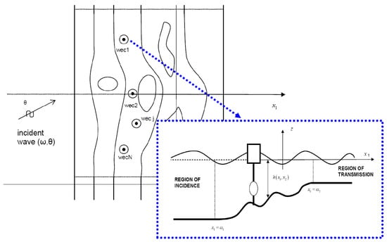
Figure 1.
Array of WECs in variable bathymetry region.
The variable bathymetry region is considered between two infinite sub-regions of constant, but possibly different depths (region of incidence) and (region of transmission). In the middle sub-region, it is assumed that the depth exhibits an arbitrary variation. The wave field is excited by a harmonic incident wave of angular frequency ω, propagating with direction θ; see Figure 1. Under the assumptions that the free-surface elevation and the wave velocities are small, the wave potential is expressed as follows:
where and satisfies the linearized water wave equations; see []. In the above equation is the incident wave height, g is the acceleration due to gravity, is the frequency parameter, and . The free surface elevation is then obtained in terms of the wave potential as follows:
Using standard floating-body hydrodynamic theory [], the complex potential can be decomposed as follows:
where is the normalized propagation wave potential in the variable bathymetry region in the absence of the WECs, is the diffraction potential due to the presence fixed (motionless) bodies , that satisfies the boundary condition on k-WEC, where the normal vector on the wetted surface of the k-body, directed outwards the fluid domain (inwards the body). Furthermore, , denotes the radiation potential in the non-uniform domain associated with the -oscillatory motion of the k-body with complex amplitude , satisfying , equal to the -component of generalized normal vector on the wetted surface of the k-WEC ( for ).
In the case of simple heaving WECs, only the vertical oscillation of each body is considered , which is one of the most powerful intensive modes concerning this type of wave energy systems. In the present work we will concentrate on this simpler configuration, leaving the analysis of the more complex case to be examined in future work. For an array of heaving WECs the hydrodynamic response is obtained by:
where denote the exciting vertical force on each WEC due to propagating and diffraction field, respectively, and the matrix coefficient is given by:
where denotes Kronecker’s delta and M is the body mass (assumed the same for all WECs). The hydrodynamic coefficients (added mass and damping) are calculated by the following integrals:
of the heaving-radiation potential of the k-WEC on the wetted surface of the m-WEC. Moreover, is the hydrostatic coefficient in heaving motion with the waterline surface, and are characteristic constants of the Power Take Off (PTO) system associated with the m-th degree of freedom of the floater. The components of the excitation (Froude-Krylov and diffraction) forces are calculated by the following integrals of the corresponding potentials:
on the wetted surface of the m-WEC. The total power extracted by the array is obtained as:
where indicates the efficiency of the PTO associated with the k-th degree of freedom (that could be a function of the frequency ω). Finally, the q-index can be estimated by:
where indicates the output of a single device operating in the same environment and wave conditions. Obviously, the calculated performance depends on the frequency, direction and height of the incident wave, as well as on the physical environment and the positioning of the WECs in the array (farm layout). Finally, the operational characteristics of the farm, in general multi chromatic wave conditions, characterized by directional wave spectrum, could be obtained by appropriate spectral synthesis; see, e.g., [,].
3. Propagating Wave Field
The wave potential associated with the propagation of water waves in the variable bathymetry region, without the presence of the scatterer (floating body), can be conveniently calculated by means of the consistent coupled-mode model developed [], as extended to three-dimensional environments by []. This model is based on the following enhanced local-mode representation:
In the above expansion, the term denotes the propagating mode of the generalized incident field. The remaining terms are the corresponding evanescent modes, and the additional term is a correction term, called the sloping-bottom mode, which properly accounts for the satisfaction of the Neumann bottom boundary condition of the non-horizontal parts of the bottom. The function represents the vertical structure of the n-th mode. The function describes the horizontal pattern of the n-th mode and is called the complex amplitude of the n-th mode. The functions , , are obtained as the eigenfunctions of local vertical Sturm-Liouville problems formulated in the local vertical intervals , and are given by:
In the above equations the eigenvalues are obtained as the roots of the local dispersion relations:
The function is defined as the vertical structure of the sloping-bottom mode. This term is introduced in the series in order to consistently satisfy the Neumann boundary condition on the non-horizontal parts of the seabed. It becomes significant in the case of seabottom topographies with non-mildly sloped parts and has the effect of significant acceleration of the convergence of the local mode series Equation (10); see []. In fact, truncation of the series (10) keeping only a small number 4–6 totally terms have been proved enough for calculating the propagating wave field in variable bathymetry regions with bottom slopes up to and exceeding 100%. For specific convenient forms of see the discussion ([]). By following the procedure described in the latter work, the coupled-mode system of horizontal equations for the amplitudes of the incident wave field propagating over the variable bathymetry region is finally obtained:
where the coefficients Amn, Bmn, Cmn of the coupled-mode system (13) are defined in terms of the vertical modes . The coefficients are dependent on through and the corresponding expressions can be found in Table 1 of []. The system is supplemented by appropriate boundary conditions specifying the incident waves and treating reflection, transmission and radiation of waves. It is worth mentioning here that if only the propagating mode (n = 0) is retained in the expansion (11) the above CMS reduces to an one-equation model which is exactly the modified mild-slope Equation derived in [,]. So, the present approach could be automatically reduced to mild-slope model in the subregions where such a simplification is permitted, saving a lot of computational cost. On the other hand in subregions where bottom variations are strong the extra (evanescent) modes are turned on and have substantial effects concerning the 3D wave field all over the water column, as illustrated in [,].

Table 1.
Optimum PML parameters.
4. A Novel BEM for the Diffraction and Radiation Problems in 3D Environments
The corresponding problems on the diffraction and radiation potentials associated with the operation of the floating WECs, are treated by means of low-order Boundary Element Method, based on simple singularity distributions and 4-node quadrilateral boundary elements ([]), ensuring continuity of the geometry approximation of the various parts of the boundary. The potential and velocity fields are approximated by:
where the summation ranges over all panels and and denote induced potential and velocity from the p-th element with unit singularity distribution to the field point r; see, e.g., [] and the references cited there. We mention here that a minimum number of 10–20 elements per wavelength is used in discretizing the free surface, in order to eliminate errors due to damping and dispersion associated with the above discrete scheme. In order to eliminate the infinite extent of the domain and treat the radiating behaviour of the diffraction and radiation fields at far distances from the bodies, an absorbing layer technique is used, based on a matched layer all around the fore and side borders of the computational domain on the free surface; see, e.g., []. The thickness of the absorbing layer is of the order of 1–2 characteristic wavelengths and its coefficient is taken increasing within the layer; see Figure 2. The efficiency of this technique to damp the outgoing waves with minimal reflection is dependent on the thickness of the layer.
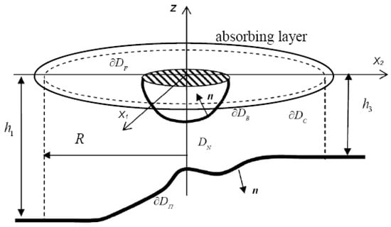
Figure 2.
Formulation of diffraction and radiation problems in variable bathymetry regions.
Thus, the diffraction and radiation potentials are represented by integral formulations with support only on the wetted surface of the floating body (ies) , the bottom surface and free surface ; see Figure 2. In accordance with the present absorbing layer model, the free surface boundary condition is modified as follows:
where and the coefficient everywhere on , except in the absorbing layer (indicated in Figure 2), where this is given by:
where λ is the local wavelength.
Also, it is assumed for the starting radius of the absorbing layer that . The discrete solution is then obtained using collocation method, by satisfying the boundary conditions at the centroid of each panel on the various parts of the boundaries. Induced potentials and velocities from each panel to any collocation point are calculated by numerical quadratures, treating the self-induced quantities semi-analytically.
4.1. Investigation of the Optimal Parameters of the Absorbing Layer
The radiation condition expresses the weakening behavior of the outgoing waves at the far field, and it formulates the final solution. In complicated problems, where analytical or even semi-analytical solutions are unreachable, this condition cannot be formed a priori and further investigation is needed, in order to obtain its final form. One common way to overcome this obstacle, is the implementation of an absorbing layer from a specific length of activation and with defined characteristics, based on the Perfectly Matched Layer (PML) model [,]. In this specific approach, the wave absorbing is induced by an imaginary part of frequency, expressed by Equations (15) and (16), which operates as a damping filter for the waves without significant reflections. The formulation of the optimal PML is a multiparametric problem, mainly based on five parameters. The objective functions of this optimization procedure is the avoidance of any influence of the PML in the region before its appliance, due to reflections, and the progressive nullification of the wave field in the region after its activation. The effectiveness of the PML can be tested by comparing the numerical and the analytical solution in case of a cylindrical WEC body in steady depth regions []. The requirement for the PML not to disturb the solution in the computational domain before its activation is quantified with the usage of the Chebyshev Norm. Thus, the PML tunning parameters, discussed above, are:
- Dimensionless frequency
- Coefficient
- The activation length
- The exponent
- The number of panels per wave length (N/λ)
Aiming to the minimization of the Chebyshev Norm, 64 different PMLs, corresponding to different sets of these parameters, are investigated. The final configuration of the optimum PML is described in Table 1. The efficient operation of the PML, especially in medium frequency bandwidths, where WEC devices operate most of the time and absorb the largest amount of energy, is illustrated in Figure 3, for different values of the non-dimensional frequency .
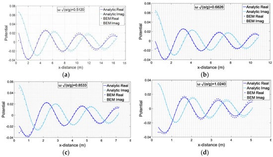
Figure 3.
Comparison of present BEM results with the analytic solution in case of cylindrical WEC a/h = 1/3.5 and d/a = 1.5dr/a = 1.5/1, where α: radius, h: local depth and d: draft, for different values of the non-dimensional frequency : (a) 0.5120; (b) 0.6826; (c) 0.8533; (d) 1.0240.
4.2. Power Output in the Case of Cylindrical WEC
A cylindrical heaving WEC is widely used in offshore installations of the devices for harnessing wave energy []. The numerical treatment of the wave-body interaction problem by means of BEM, described in this study, constitutes from three separate regions, namely the free surface, the body of the WEC and the bottom. Appropriate mesh generation in all these surfaces is crucial for obtaining reliable solution. For this purpose, the free surface is discretized in 4 × (N/λ) × 88 elements, expanding for 4 wavelengths, where the first number indicates discretization along the radial direction and the other along azimuthal direction, respectively, while the bottom mesh is 26 × 88 elements, spatially and azimuthally respectively. The WEC mesh is 10 × 88 elements, in depth and in azimuthal direction, as illustrated in Figure 4. It should be noticed the demand for consistency between the lengths of the elements, those of the WEC and these of the free surface, at the matching position of the body’s boundary. Very fine meshes only on the body and not on the free surface, which binds most of the computational capacity and therefore has its limitations, may cause worse approximation of the analytic solution on account of inconsistency.
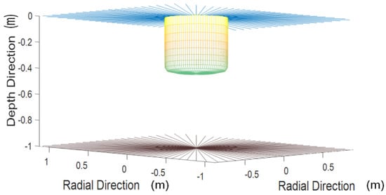
Figure 4.
Illustration of the computational mesh in the near field. For clarity only the radial lines of the mesh on the free surface and on the bottom surface under the floater are shown.
Focusing on the power output coming from a single device, the first step for its calculation is the evaluation of the Froude-Krylov and total forces, which are the summation of Froude-Krylov and Diffraction forces, and the related hydrodynamic coefficients of added mass and damping. In Figure 5 and Figure 6 are illustrated the results for these aspects, as they calculated both from the analytical and the numerical treatment of the problem ([,]).
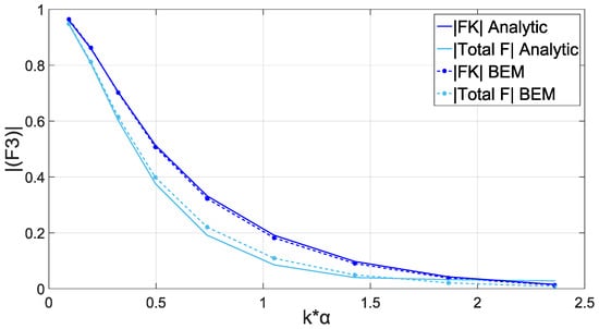
Figure 5.
Non-dimensionalized cylinder hydrodynamic Froude-Krylov and total forces for various values of non-dimensionalized wavenumber (kα). Cylindrical WEC with and .
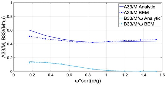
Figure 6.
Non-dimensionalized cylinder hydrodynamic coefficients for various values of non-dimensionalized frequency. Cylindrical WEC with and .
Furthermore, the WEC responses and the power output are evaluated and plotted in Figure 7, assuming typical PTO damping values, equal to 5, 10 and 20 times a mean value of hydrodynamic damping bm. This value is estimated as , where the resonance frequency is , also described in [].
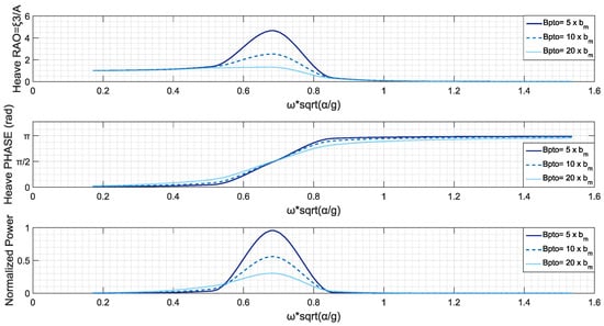
Figure 7.
Heave Response amplitude operator (RAO) RAO, Phase RAO and Normalized Power Output for Cylindrical WEC with and .
The output power of the WEC by this PTO is normalized with respect to the incident wave powerflux and is defined as , for . It can be observed the fact that maximization of power output occurs at the resonance frequency. In addition, higher values of PTO damping are reasons for the observed decrease of peak values of heave Response Amplitude Operator (defined as , where a is the amplitude of the incident wave). However, at the same time they are causing wider frequency spreads of energy productive function of the device.
5. Examination of Other Shapes of Axisymmetric Floaters
Regarding the examination of other WEC shapes, eight different axisymmetric geometries, including the cylinder, are tested. This is made with the conviction of efficiency improvement, in comparison with the reference cylindrical shape. Upon mesh generation, the elements used on the bodies, except cylinder, are 18 × 88, in order to achieve a better approximation of the shape, avoiding gaps and discontinuities of the geometry. For these shapes, there are no analytic solutions, and furthermore, not any prospect for validation by comparing this numerical model with analytical results. The reference cylindrical WEC has a ratio of radius to local depth, equal to 1/3.5 and a ratio of draft to radius equal to 1.5/1. In every other design test, the radius and the draft of each geometry are calculated with the assumption of constant mass. In other words, the area of the submerged vertical cross section of the tested geometry is equal to the area of the submerged vertical cross section of the cylindrical WEC, keeping with this approach the value of the mass unchangeable.
As referred previously, eight different shapes are put under investigation. Heave response and power output are evaluated by the BEM computational code. These geometries, illustrated in Figure 8, are strongly related with the current design trends of the industry and present similarities with many already installed WEC devices [,,,].
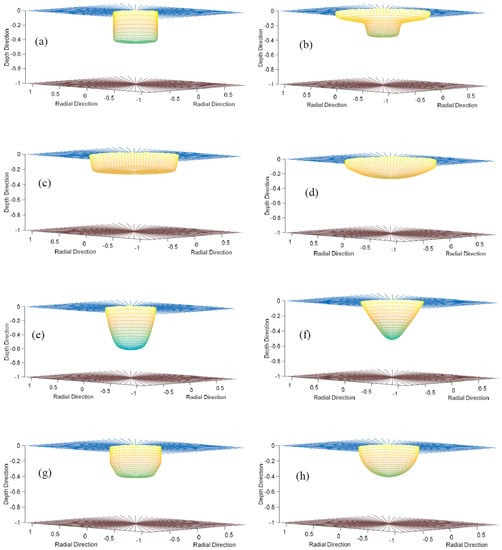
Figure 8.
Various WEC shapes and near field computational mesh: (a) Cylindrical, (b) Nailhead-shaped, (c) Disk-shaped, (d) Elliptical, (e) Egg-shaped, (f) Conical, (g) Floater-shaped, (h) Semi-spherical.
Using as an efficiency index, the area under the curve of the normalized power, which expresses the maximum values so as the functional frequency bandwidth, three of the above geometries are qualified and their heave response and power output are presented in Figure 9, Figure 10 and Figure 11. The qualified geometries are namely the nailhead-shaped, which also presents further interest due to its unconventional design for studies of multi-dof WECs, the conical and the floater-shaped.
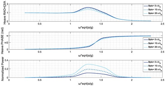
Figure 9.
Heave RAO, Phase RAO and Normalized Power Output-Nailhead-shaped WEC.
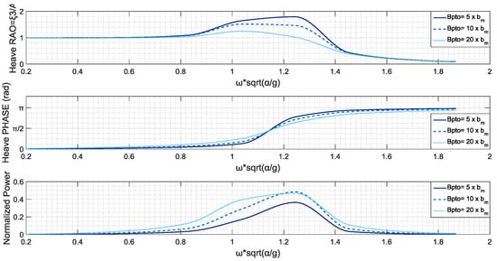
Figure 10.
Heave RAO, Phase RAO and Normalized Power Output-Conical WEC.
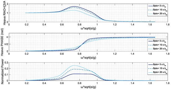
Figure 11.
Heave RAO, Phase RAO and Normalized Power Output-Floater-shaped WEC.
On the assessment of these geometries, according to the figures above, despite the fact that the PTO with higher damping is responsible for lower values of heave RAO, the power output appears to be higher and with a higher frequency spreading. This dissimilar behavior of the device, in terms of heave RAO and power output, is very intense in case of the nailhead-shaped WEC, where RAOs are closely oriented, while the power output is far higher in the case of the “harder” PTO. A point of interest in the study of the conical WEC is that a switch of efficiency occurs in , when the medium ranked PTO is more efficient than higher ranked. Furthermore, the floater-shaped WEC is shown to be a little more efficient in lower frequencies, where the maximum of the power output curve is located, while the nailhead-shaped and the conical are more efficient in bandwidths of 11 < < 1.4. The conical WEC is far more efficient in frequencies of 0.9 < < 1.4, however, the final choice of the device and the PTO is depended on the sea climate and the dominant frequencies in the area of installation.
6. Extensions to Treat the WEC Arrays in Variable Bathymetry Regions
An important part of the present BEM implementation deals with the construction of the mesh on the various parts of the boundary. The details of the mesh generator are illustrated in Figure 12. More specifically, the mesh on the free surface around a single WEC is plotted. The latter consists of two subparts, the one close to the waterline of the floating unit and the far (outer) part. The near mesh is based on the cylindrical distribution of the panels around the waterline of the WEC that gradually deforms in order to end in a rectangular boundary. This permits the continuous junction of the near mesh around one floater with the adjacent one, as illustrated in Figure 12a. After the rectangular boundary, the mesh again deforms to become a cylindrical arrangement on the outer part. Taking into account that in 3D diffraction and radiation fields associated with floating bodies the far field behaves like essentially cylindrical outgoing waves [], the cylindrical mesh in the outer part of the free surface boundary is considered to be optimum for the numerical solution of the studied problems. The discretization is accomplished by the incorporation corresponding meshes on each floating body and on the bottom variable bathymetry surface, as shown in Figure 12b–d. An important feature is the continuous junction of the various parts of the mesh, which, in conjunction with the quadrilateral elements, ensures global continuity of the geometry approximation of the boundary. It is remarked here that the present BEM is free of any kind of interior meshes or artificial intesection(s) of boundaries. Global continuity of geometry is important concerning the convergence of the numerical results in BEM.
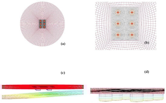
Figure 12.
Computational grid for a WEC array of 3 × 2 WECs: (a) plot of the whole mesh on the free surface, (b) zoom in the subregion of floaters, (c,d) 3D view of the mesh in the vicinity of the WECs.
As an example, we consider the array of 3 × 2 cylindrical heaving WECs of radius a = 10 m and draft d/a = 1.5, arranged as illustrated in Figure 12, in the middle of the variable bathymetry region (a smooth upslope with max bottom slope 7%), and operating in waves at the same frequency as before , . The horizontal spacing of the floaters along the and axes is . In this case the ratio of the WEC spacing with respect to the characteristic wavelength in the area of the array is small (less than 50%) and thus, the interaction between the floaters is strong. In order to illustrate the applicability of the present BEM, a mesh is used, consisting of 6 × 40 elements on each WEC and 5 × 40 elements on the nearest part of the free surface around each WEC and 30 × 100 elements on the outer part. This includes the absorbing layer, and 14 × 20 elements on the bottom surface (see Figure 12). The total number of elements is 5920.
The propagating field over the shoaling region, for normally and for 45deg obliquely incident waves is shown in Figure 13. This field represents the available wave energy in the domain for possible extraction. The responses of the above array of cylindrical heaving WECs are then calculated, using, as before, the values of = 5, 10, 20 (where ) to model the Power Take Off system for heving floaters. The results calculated by the present BEM approach, at the same frequency as before , , both for normal and 4deg incident waves over the variable bathymetry region are represented in Figure 14. In the specific arrangement and operating conditions the q-factor decreases with increasing PTO damping and ranges from 90–70%, for normal incident waves, and drops down to 75–60%, for 45 degrees obliquely incident waves.
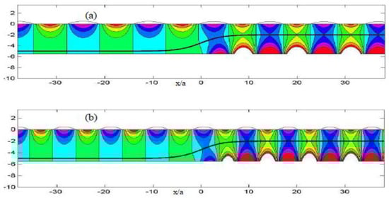
Figure 13.
(a) Propagating field over a shoaling region, for normally incident waves of nondimensional frequency . (b) Same as before, but for 45 degrees obliquely incident waves.
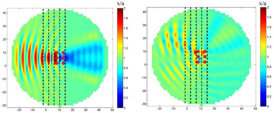
Figure 14.
Total field of the WEC array for (a) normal and (b) 45 degrees incidence (right) and , , in the variable bathymetry region (dashed lines represent depth contours). The colorbar indicates relative intensity of the wavefield.
7. Conclusions
In this work a numerical method is presented for the hydrodynamic analysis of the floating bodies over general seabed topography supporting the calculation of the wave power absorption by single WECs and the performance of arrays of devices in nearshore and coastal regions. As a first step, in order to subsequently formulate and solve 3D diffraction and radiation problems for floaters in the inhomogeneous domain, the present approach is based on the coupled-mode model for the calculation of the wave field propagating over the variable bathymetry region. The results are subsequently used for the hydrodynamic analysis of floating bodies over general bottom topography by means of a low-order BEM. Extensions of the present method supporting the estimation of single WEC and WEC array performance in variable bathymetry regions have been discussed. Future work will be focused on the validation of the present method by comparisons with other methods and experimental laboratory data. Moreover, phase-averaged models like SWAN can treat macroscopically WEC-array effects by including energy pumping in the energy balance equations by using sinks with specific intensity; see, e.g., []. Future work will examine the possibility of coupling phase-averaged with the present phase-resolving model, by using coupling schemes as the ones presented in [,] and present comparisons at the scale of an array in a nearshore region.
Author Contributions
The main ideas of this work as well as the first draft of the text belong to Kostas Belibassakis. Markos Bonavos participated in performing the numerical simulations and writing some parts of the text. Eugen Rusu suggested improvements and performed several corrections and verification of the text and of the Figures. He was also the corresponding author and his work is included in a Romanian national research project as stated in Acknowledgments. All authors agreed with the final form of this article.
Funding
This research received no external funding.
Acknowledgments
The work of the corresponding author was carried out in the framework of the research project REMARC (Renewable Energy extraction in MARine environment and its Coastal impact), supported by the Romanian Executive Agency for Higher Education, Research, Development and Innovation Funding – UEFISCDI, grant number PN-III-P4-IDPCE-2016-0017.
Conflicts of Interest
The authors declare no conflict of interest.
Abbreviations
| BEM | Boundary Element Method |
| CMS | Coupled-Mode System |
| RAO | Response amplitude operator |
| PML | Perfectly Matched Layer |
| PTO | Power Take off |
| SWAN | Simulating Waves Nearshore |
| WEC | Wave Energy Converters |
References
- Mei, C.C. The Applied Dynamics of Ocean Surface Waves, 2nd ed.; World Scientific: Singapore, 1996. [Google Scholar]
- Sawaragi, T. Coastal Engineering-Waves, Beaches, Wave-Structure Interactions, 1st ed.; Elsevier: Amsterdam, The Netherlands, 1995. [Google Scholar]
- Williams, K.J. The boundary integral equation for the solution of wave–obstacle interaction. Int. J. Numer. Method. Fluids 1988, 8, 227–242. [Google Scholar] [CrossRef]
- Drimer, N.; Agnon, Y.; Stiassnie, M. A simplified analytical model for a floating breakwater in water of finite depth. Appl. Ocean Res. 1992, 14, 33–41. [Google Scholar] [CrossRef]
- Williams, A.N.; Lee, H.S.; Huang, Z. Floating pontoon breakwaters. Ocean Eng. 2000, 27, 221–240. [Google Scholar] [CrossRef]
- Drobyshevski, Y. Hydrodynamic coefficients of a two-dimensional, truncated rectangular floating structure in shallow water. Ocean Eng. 2004, 31, 305–341. [Google Scholar] [CrossRef]
- Drobyshevski, Y. An efficient method for hydrodynamic analysis of a floating vertical-sided structure in shallow water. In Proceedings of the 25th International Conference on Offshore Mechanics and Arctic Engineering (OMAE2006), Hamburg, Germany, 4–9 June 2006. [Google Scholar]
- Wehausen, J.V. The motion of floating bodies. Ann. Rev. Fluid. Mech. 1971, 3, 237–268. [Google Scholar] [CrossRef]
- Wehausen, J.V. Methods for Boundary-Value Problems in Free-Surface Flows: The Third David W. Taylor Lecture, 27 August through 19 September 1974. Available online: https://www.researchgate.net/publication/235068177_Methods_for_Boundary-Value_Problems_in_Free-Surface_Flows_The_Third_David_W_Taylor_Lecture_27_August_through_19_September_1974 (accessed on 15 July 2018).
- Charrayre, F.; Peyrard, C.; Benoit, M.; Babarit, A. A coupled methodology for wave body interactions at the scale of a farm of wave energy converters including irregular bathymetry. In Proceedings of the 33th International Conference on Offshore Mechanics and Arctic Engineering (OMAE2014), San Francisco, CA, USA, 8–13 June 2014. [Google Scholar]
- McCallum, P.; Venugopal, V.; Forehand, D.; Sykes, R. On the performance of an array of floating energy converters for different water depths. In Proceedings of the 33th International Conference on Offshore Mechanics and Arctic Engineering (OMAE2014), San Francisco, CA, USA, 8–13 June 2014. [Google Scholar]
- Guazzelli, E.; Rey, V.; Belzons, M. Higher-order bragg reflection of gravity surface waves by periodic beds. J. Fluid Mech. 1992, 245, 301–317. [Google Scholar] [CrossRef]
- Massel, S. Extended refraction-diffraction equations for surface waves. Coast. Eng. 1993, 19, 97–126. [Google Scholar] [CrossRef]
- Rey, V. A note on the scattering of obliquely incident surface gravity waves by cylindrical obstacles in waters of finite depth. Eur. J. Mech. B/Fluid 1995, 14, 207–216. [Google Scholar]
- Belibassakis, K.A. A Boundary Element Method for the hydrodynamic analysis of floating bodies in general bathymetry regions. Eng. Anal. Bound. Elem. 2008, 32, 796–810. [Google Scholar] [CrossRef]
- Touboul, J.; Rey, V. Bottom pressure distribution due to wave scattering near a submerged obstacle. J. Fluid Mech. 2012, 702, 444–459. [Google Scholar] [CrossRef]
- Athanassoulis, G.A.; Belibassakis, K.A. A consistent coupled-mode theory for the propagation of small-amplitude water waves over variable bathymetry regions. J. Fluid Mech. 1999, 389, 275–301. [Google Scholar] [CrossRef]
- Belibassakis, K.A.; Athanassoulis, G.A.; Gerostathis, T. A coupled-mode system for the refraction-diffraction of linear waves over steep three dimensional topography. Appl. Ocean. Res. 2001, 23, 319–336. [Google Scholar] [CrossRef]
- Magne, R.; Belibassakis, K.A.; Herbers, T.; Ardhuin, F.; O’Reilly, W.C.; Rey, V. Evolution of surface gravity waves over a submarine canyon. J. Geogr. Res. 2007, 112, C01002. [Google Scholar] [CrossRef]
- Gerostathis, T.; Belibassakis, K.A.; Athanassoulis, G.A. A coupled-mode model for the transformation of wave spectrum over steep 3D topography: Parallel-Architecture Implementation. J. Offshore Mech. Arct. Eng. 2008, 130. [Google Scholar] [CrossRef]
- Belibassakis, K.A.; Athanassoulis, G.A. A coupled-mode system with application to nonlinear water waves propagating in finite water depth and in variable bathymetry regions. Coast. Eng. 2011, 58, 337–350. [Google Scholar] [CrossRef]
- Belibassakis, K.A.; Athanassoulis, G.A.; Gerostathis, T. Directional wave spectrum transformation in the presence of strong depth and current inhomogeneities by means of coupled-mode model. Ocean Eng. 2014, 87, 84–96. [Google Scholar] [CrossRef]
- Vincent, C.L.; Briggs, M.J. Refraction–diffraction of irregular waves over a mound. J. Waterw. Port Coast. Ocean Eng. 1989, 115, 269–284. [Google Scholar] [CrossRef]
- Booij, N.; Ris, R.C.; Holthuijsen, L.H. A third-generation wave model for coastal regions, 1. Model description and validation. J. Geophys. Res. 1999, 104, 7649–7666. [Google Scholar] [CrossRef]
- Ris, R.C.; Holthuijsen, L.H.; Booij, N. A Third-Generation Wave Model for Coastal Regions. Verification. J. Geophys. Res. 1999, 104, 7667–7681. [Google Scholar] [CrossRef]
- Belibassakis, K.A.; Athanassoulis, G.A. Three-dimensional Green’s function of harmonic water-waves over a bottom topography with different depths at infinity. J. Fluid Mech. 2004, 510, 267–302. [Google Scholar] [CrossRef]
- Massel, S.R. Ocean Surface Waves. Their Physics and Prediction; World Scientific: Singapore, 2013. [Google Scholar]
- Chamberlain, P.G.; Porter, D. The modified mild-slope equation. J. Fluid Mech. 1995, 291, 393–407. [Google Scholar] [CrossRef]
- Beer, G.; Smith, I.; Duenser, C. The Boundary Element Method with Programming for Engineers and Scientists; Springer: New York, NY, USA, 2008; ISBN 978-3-211-71576-5. [Google Scholar]
- Teng, B.; Gou, Y. BEM for wave interaction with structures and low storage accelerated methods for large scale computation. J. Hydrodyn. 2017, 29, 748–762. [Google Scholar] [CrossRef]
- Sclavounos, P.; Borgen, H. Seakeeping analysis of a high- speed monohull with a motion control bow hydrofoil. J. Ship Res. 2004, 48, 77–117. [Google Scholar]
- Berenger, J.P. A perfectly matched layer for the absorption of electromagnetic waves. J. Comput. Phys. 1994, 114, 185–200. [Google Scholar] [CrossRef]
- Turkel, E.; Yefet, A. Absorbing PML boundary layers for wave-like equations. Appl. Numer. Math. 1998, 27, 533–557. [Google Scholar] [CrossRef]
- Sabuncu, T.; Calisal, S. Hydrodynamic coefficients for vertical circular cylinders at finite depth. Ocean Eng. 1981, 8, 25–63. [Google Scholar] [CrossRef]
- Falcão, A.F. Wave energy utilization. A review of the technologies. Renew. Sustain. Energy Rev. 2010, 14, 899–918. [Google Scholar] [CrossRef]
- Filippas, E.S.; Belibassakis, K.A. Hydrodynamic analysis of flapping-foil thrusters operating beneath the free surface and in waves. Eng. Anal. Bound. Elem. 2014, 41, 47–59. [Google Scholar] [CrossRef]
- Drew, B.; Plummer, A.R.; Sahinkaya, M.N. A review of wave energy converter technology. Proc. Inst. Mech. Eng. Part A J. Power Energy 2009, 223, 887–902. [Google Scholar] [CrossRef]
- Faizal, M.; Ahmed, M.R.; Lee, Y. A Design Outline for Floating Point Absorber Wave Energy Converters. Adv. Mech. Eng. 2014, 6. [Google Scholar] [CrossRef]
- Rusu, E.; Onea, F. A review of the technologies for wave energy extraction. Clean. Energy 2018, 2. [Google Scholar] [CrossRef]
- Ruehl, K.; Porter, A.; Chartrand, C.; Smith, H.; Chang, G.; Roberts, J. “Development, Verification and Application of the SNL-SWAN Open Source Wave Farm Code”. In Proceedings of the 11th European Wave and Tidal Energy Conference EWTEC, Nantes, France, 6–11 September 2015. [Google Scholar]
- Athanassoulis, G.A.; Belibassakis, K.A.; Gerostathis, T. The POSEIDON nearshore wave model and its application to the prediction of the wave conditions in the nearshore/coastal region of the Greek Seas. Glob. Atmos. Ocean Syst. (GAOS) 2002, 8, 101–117. [Google Scholar] [CrossRef]
- Rusu, E.; Guedes Soares, C. Modeling waves in open coastal areas and harbors with phase resolving and phase averaged models. J. Coast. Res. 2013, 29, 1309–1325. [Google Scholar] [CrossRef]
© 2018 by the authors. Licensee MDPI, Basel, Switzerland. This article is an open access article distributed under the terms and conditions of the Creative Commons Attribution (CC BY) license (http://creativecommons.org/licenses/by/4.0/).