Computational Modeling of Gurney Flaps and Microtabs by POD Method


Abstract
1. Introduction
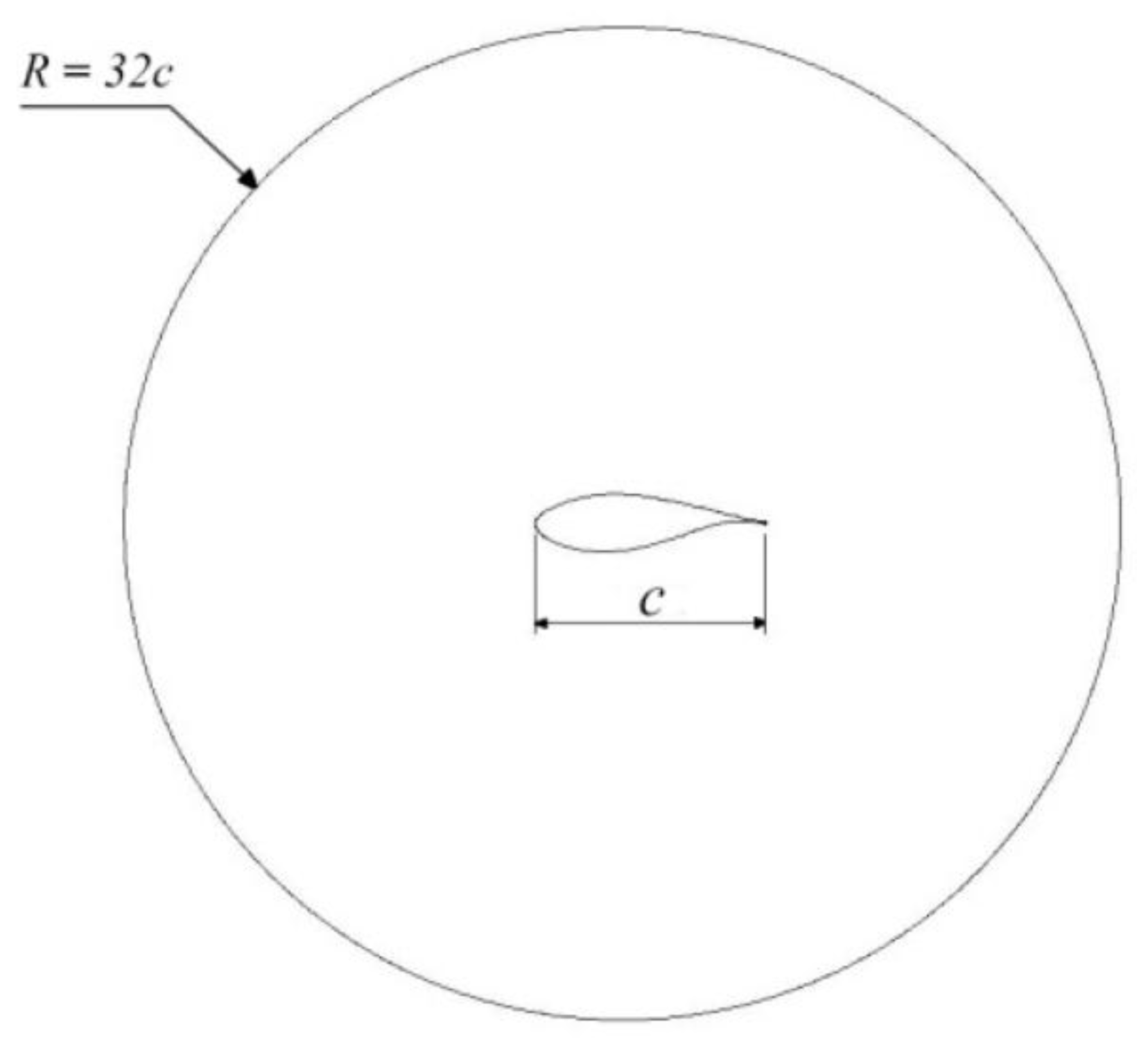
2. Numerical Setup
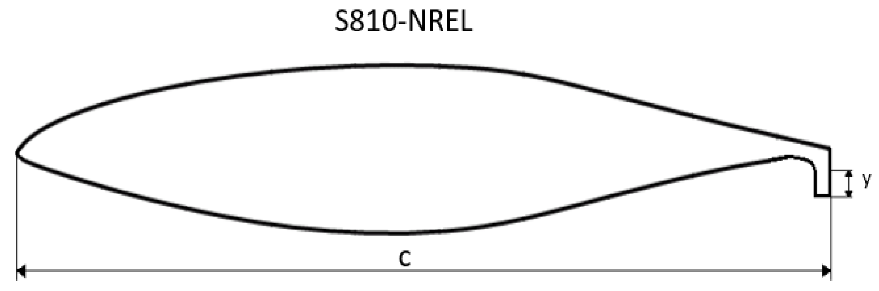
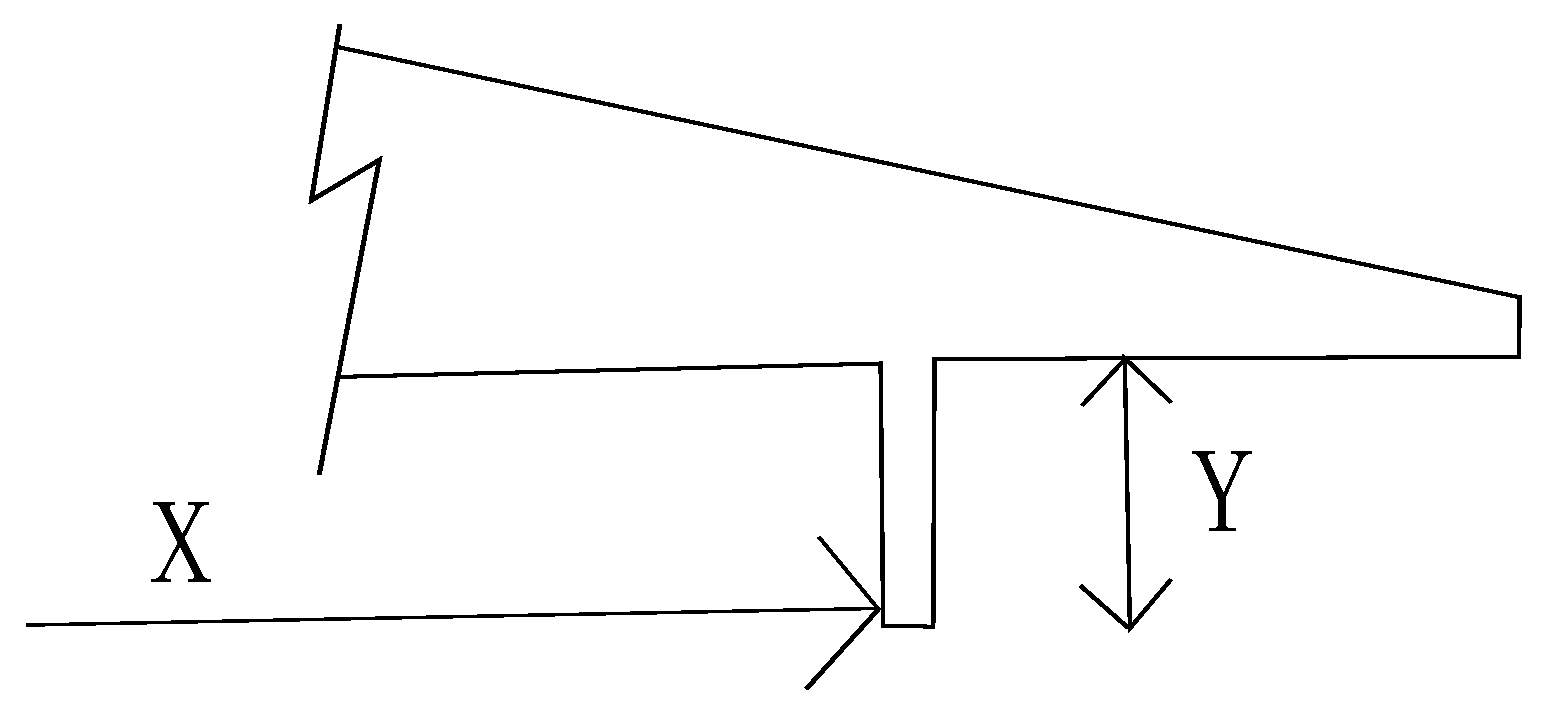
2.1. Gurney Flap Lay-Out
2.2. Microtab Layout
3. POD Method
4. Results
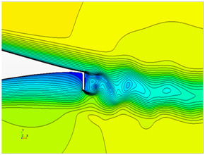
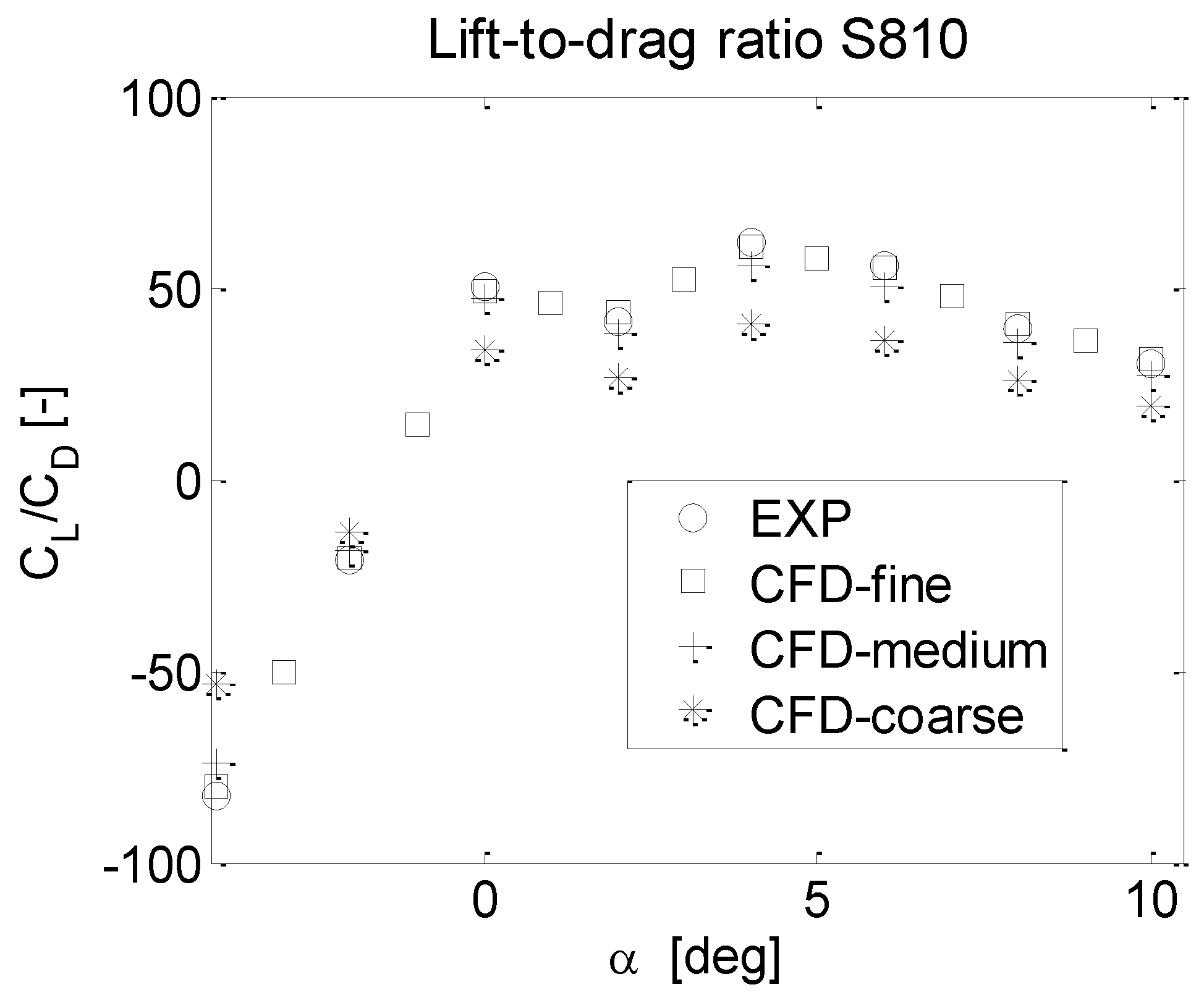
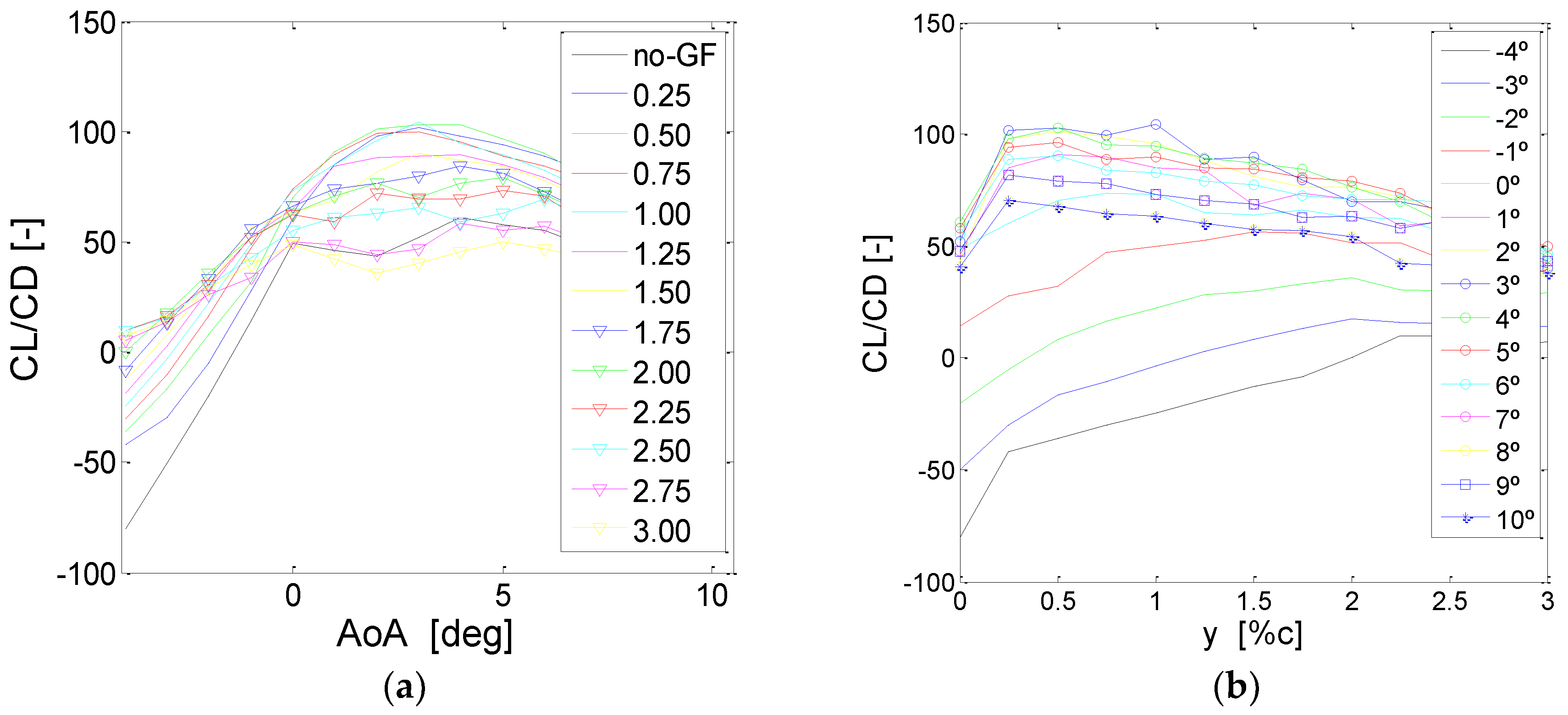
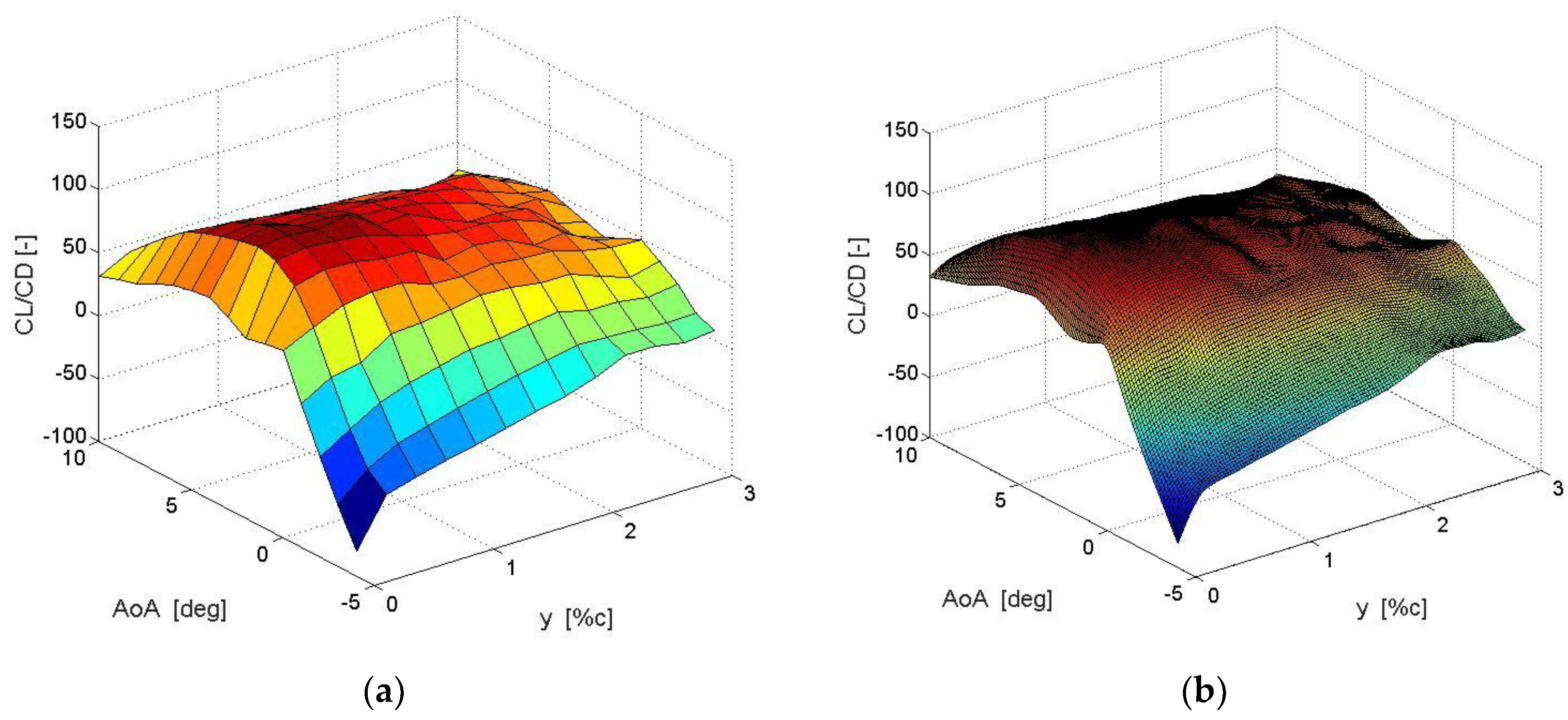
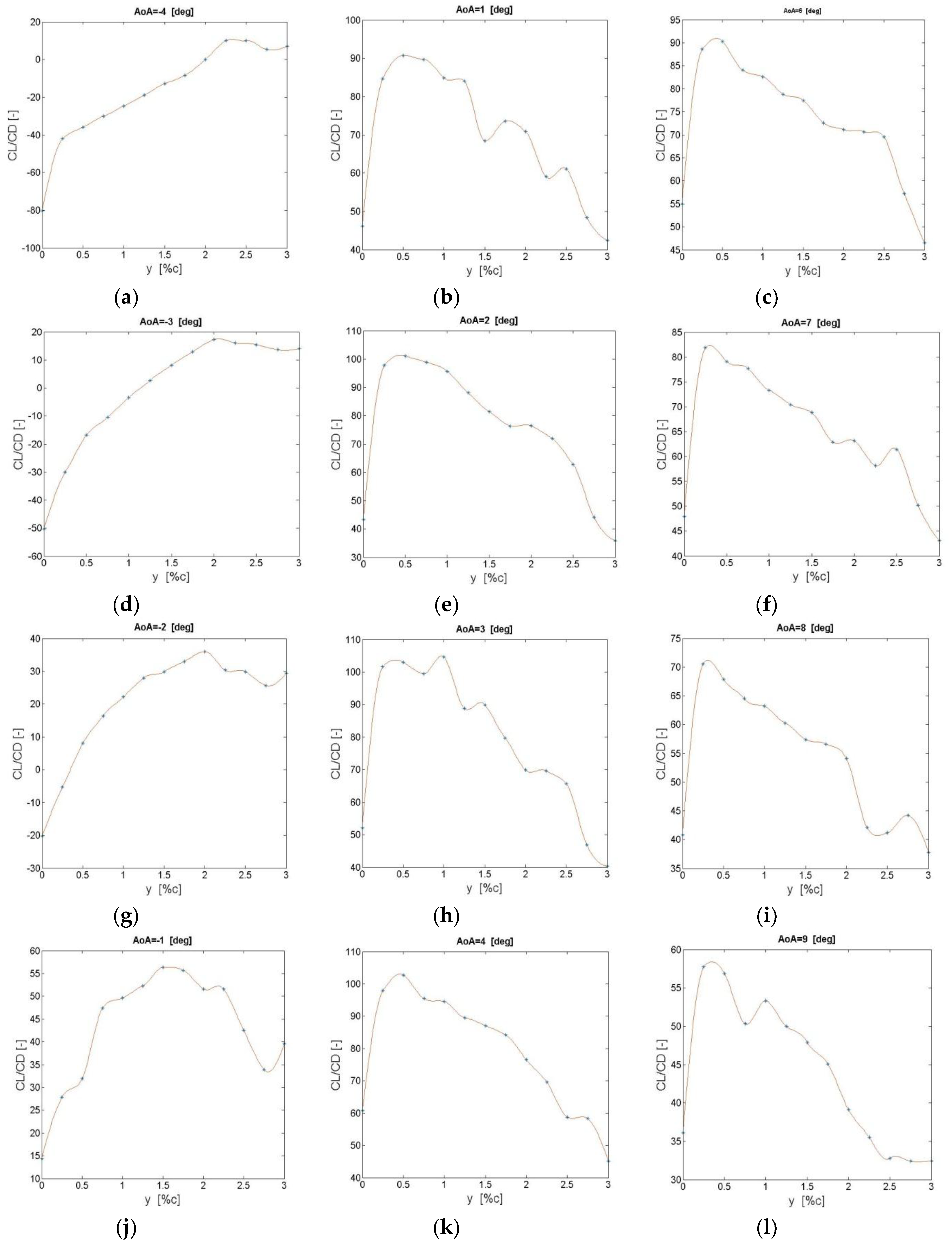
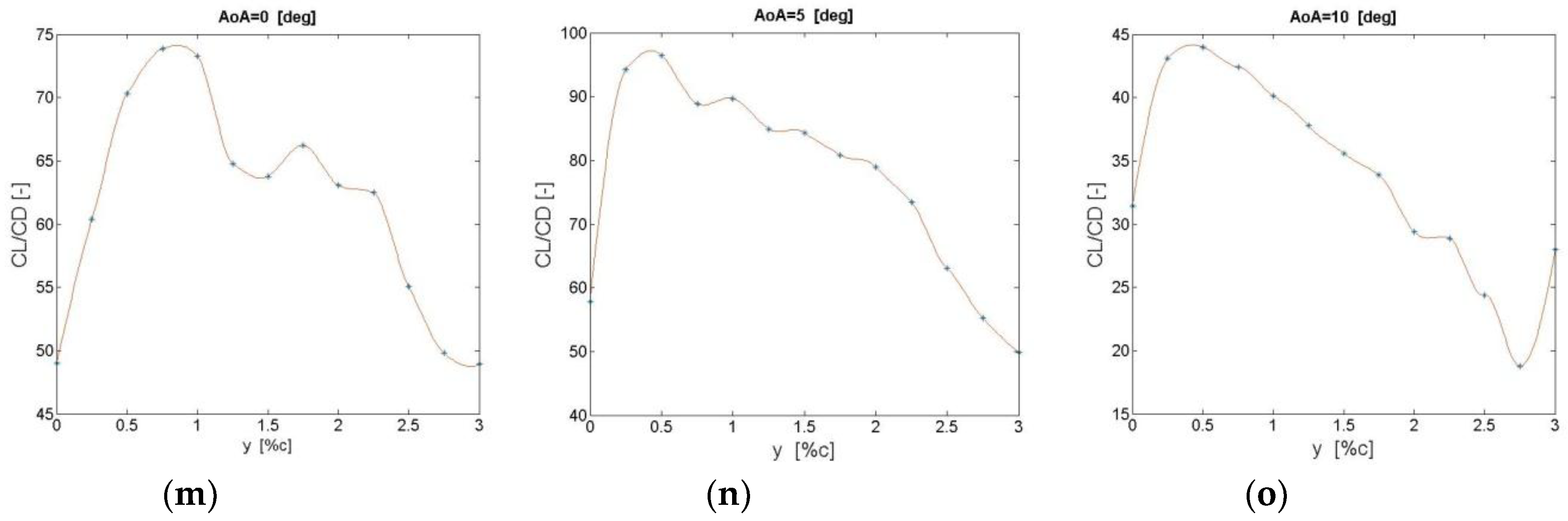
4.1. Gurney Flaps
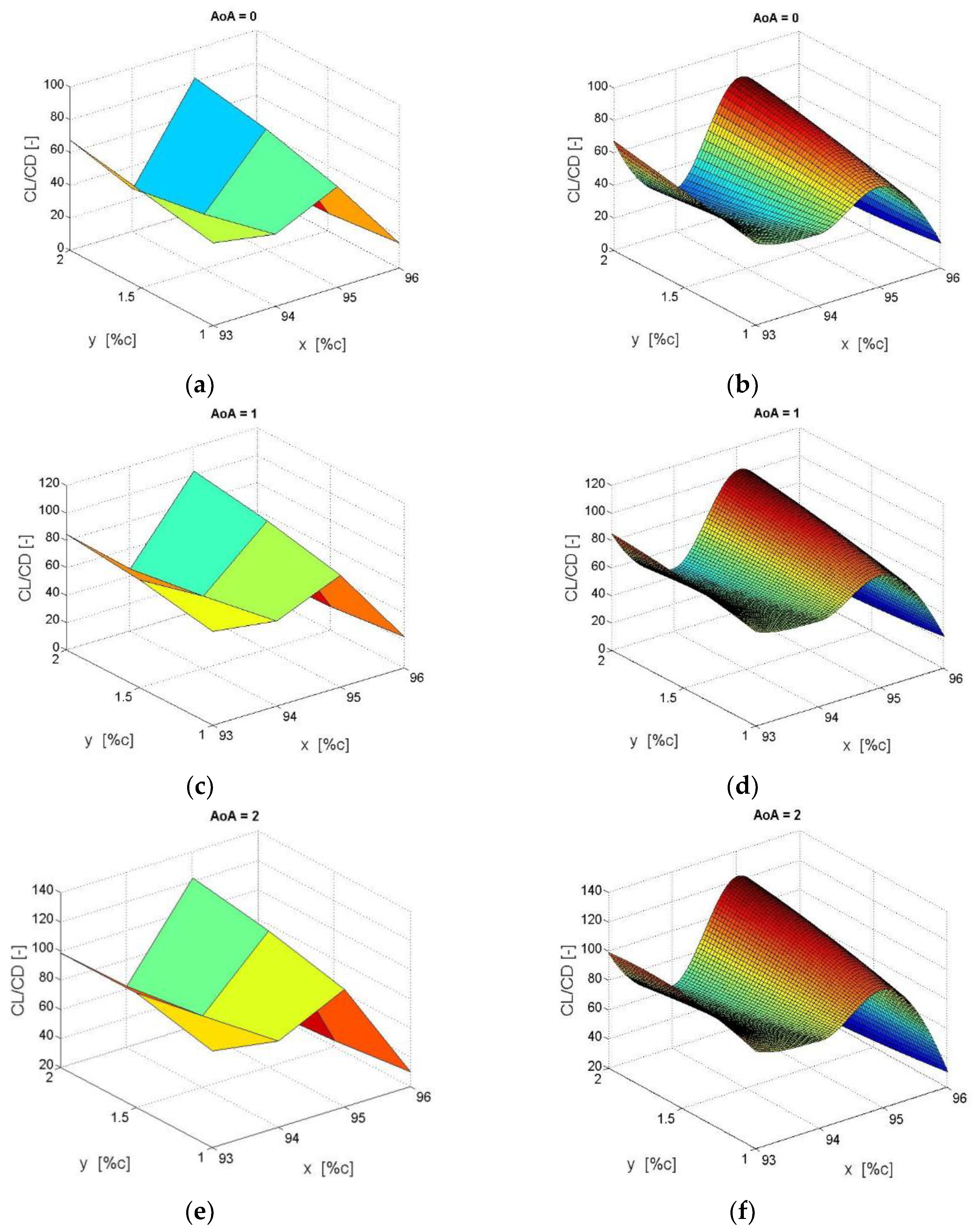
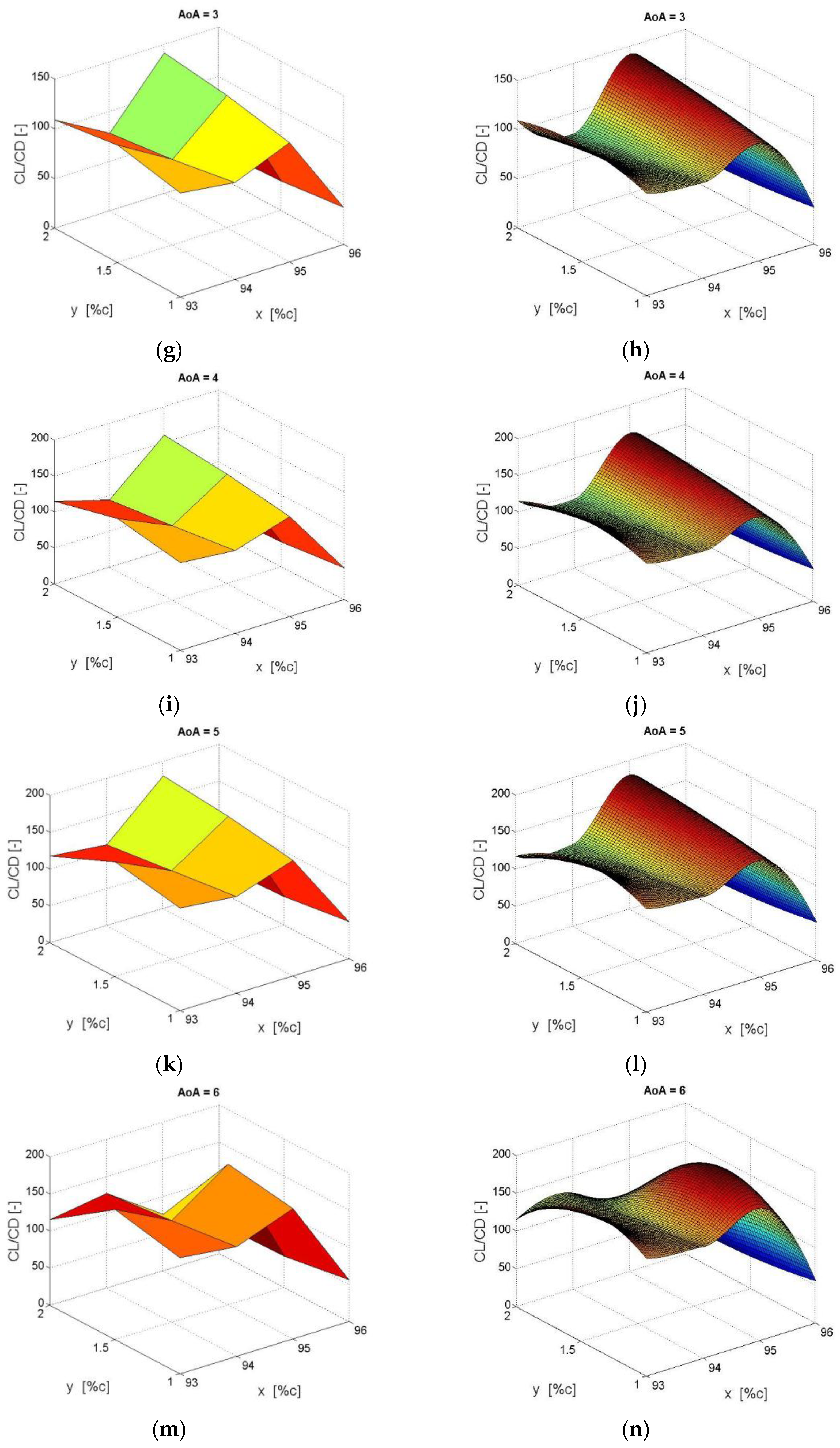
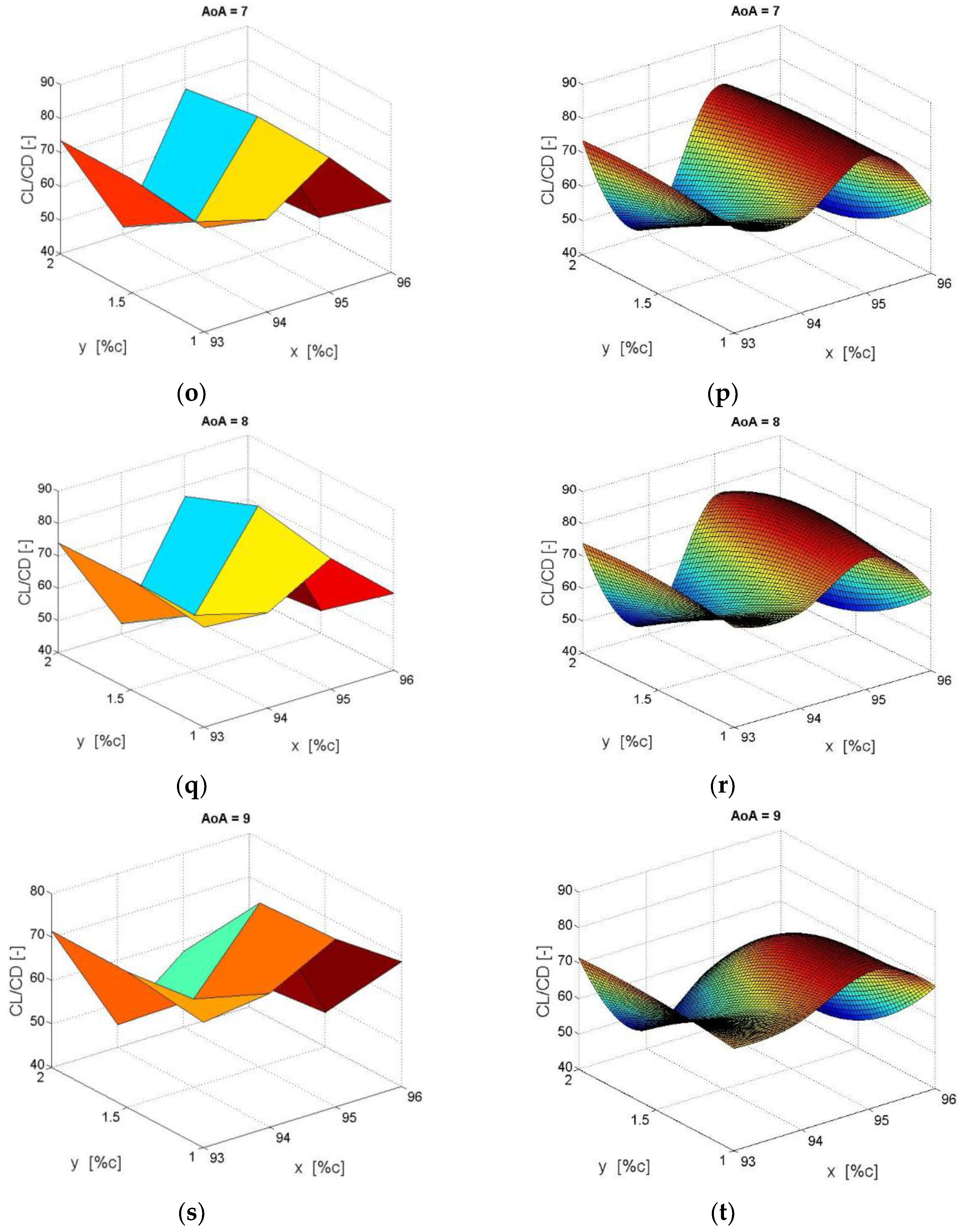
4.2. Microtabs
5. Conclusions
Author Contributions
Funding
Acknowledgments
Conflicts of Interest
Nomenclature
| CFD | Computational Fluid Dynamics |
| BEM | Blade Element Momentum |
| GF | Gurney Flap |
| MT | Microtab |
| POD | Proper Orthogonal Decomposition |
| SVD | Singular Value Decomposition |
| PCA | Principal Components Analysis |
| ROM | Reduced Order Method |
| NREL | National Renewable Energy Laboratory |
| RANS | Reynolds Averaged Navier–Stokes |
| SST | Shear Stress Transport |
| PIV | Particle Image Velocimetry |
| AoA | Angle of Attack |
| Re | Reynolds number |
Appendix A


Appendix B


References
- Johnson, S.J.; Dam, C.P. Active Load Control Techniques for Wind Turbines; Technical Report; Sandia National Laboratories: Livermore, CA, USA, August 2008. [Google Scholar]
- Baek, P.; Gaunaa, M. Modeling the temporal response of a microtab in an aeroelastic model of a wind turbine. In Proceedings of the 49th AIAA Aerospace Sciences Meeting including the New Horizons Forum and Aerospace Exposition, Orlando, FL, USA, 4–7 January 2011. [Google Scholar]
- Barlas, T.K.; Kuik, G.A.M. Review of state of the art in smart rotor control research for wind turbines. Prog. Aerosp. Sci. 2010, 46, 1–27. [Google Scholar] [CrossRef]
- Wood, R.M. A Discussion of Aerodynamic Control Effectors Concepts (ACEs) for Future Unmanned Air Vehicles (UAVs). In Proceedings of the AIAA 1st Technical Conference and Workshop on Unmanned Aerospace Vehicle, Systems, Technologies, and Operations, Portsmouth, VA, USA, 20–23 May 2002. [Google Scholar]
- Aramendia, I.; Fernandez-Gamiz, U.; Ramos-Hernanz, J.; Sancho, J.; Lopez-Guede, J.; Zulueta, E. Flow Control Devices for Wind Turbines. In Energy Harvesting and Energy Efficiency: Technology, Methods, and Applications; Bizon, N., Mahdavi Tabatabaei, N., Blaabjerg, F., Kurt, E., Eds.; Springer: Berlin, Germany, 2017; pp. 629–655. [Google Scholar]
- Aramendia-Iradi, I.; Fernandez-Gamiz, U.; Sancho-Saiz, J.; Zulueta-Guerrero, E. State of the art of active and passive flow control devices for wind turbines. Dyna 2016, 91, 512–516. [Google Scholar] [CrossRef]
- Johnson, S.J.; Baker, J.P.; van Dam, C.P.; Berg, D. An overview of active load control techniques for wind turbines with an emphasis on microtabs. Wind Energy 2010, 13, 239–253. [Google Scholar] [CrossRef]
- Frederick, M.; Kerrigan, E.C.; Graham, J.M.R. Gust alleviation using rapidly deployed trailing-edge flaps. J. Wind Eng. Ind. Aerodyn. 2010, 98, 712–723. [Google Scholar] [CrossRef]
- Woodgate, M.A.; Pastrikakis, V.A.; Barakos, G.N. Rotor computations with active gurney flaps. Presented at the ERCOFTAC Symposium on Unsteady Separation in Fluid-Structure Interaction, Mykonos, Greece, 17–21 June 2013; pp. 133–166. [Google Scholar]
- Pastrikakis, V.A.; Steijl, R.; Barakos, G.N. Effect of active gurney flaps on overall helicopter flight envelope. Aeronaut. J. 2016, 120, 1230–1261. [Google Scholar] [CrossRef]
- Wang, J.J.; Li, Y.C.; Choi, K.-S. Gurney flap-lift enhancement, mechanisms and applications. Prog. Aerosp. Sci. 2008, 44, 22–47. [Google Scholar] [CrossRef]
- Liebeck, R.H. Design of Subsonic Airfoils for High Lift. J. Aircr. 1978, 15, 547–561. [Google Scholar] [CrossRef]
- Jeffrey, D.; Zhang, X.; Hurst, D.W. Aerodynamics of gurney flaps on a single-element high-lift wing. J. Aircr. 2000, 37, 295–301. [Google Scholar] [CrossRef]
- Lee, T.; Su, Y.Y. Lift enhancement and flow structure of airfoil with joint trailing-edge flap and gurney flap. Exp. Fluids 2010, 50, 1671–1684. [Google Scholar] [CrossRef]
- Tang, D.; Dowell, E.H. Aerodynamic loading for an airfoil with an oscillating gurney flap. J. Aircr. 2007, 44, 1245–1257. [Google Scholar] [CrossRef]
- Camocardi, M.; Marañon, J.; Delnero, J.; Colman, J. Experimental study of a naca 4412 airfoil with movable gurney flap. In Proceedings of the 49th AIAA Aerospace Sciences Meeting including the New Horizons Forum and Aerospace Exposition, Orlando, FL, USA, 4–7 January 2011. [Google Scholar]
- Lee, T. Piv study of near-field tip vortex behind perforated gurney flaps. Exp. Fluids 2010, 50, 351–361. [Google Scholar] [CrossRef]
- Cole, J.A.; Vieira, B.A.O.; Coder, J.G.; Premi, A.; Maughmer, M.D. Experimental Investigation into the Effect of Gurney Flaps on Various Airfoils. J. Aircr. 2013, 50, 1287–1294. [Google Scholar] [CrossRef]
- Liu, L.; Padthe, A.K.; Friedmann, P.P. Computational study of microflaps with application to vibration reduction in helicopter rotors. AIAA J. 2011, 49, 1450–1465. [Google Scholar] [CrossRef]
- Min, B.-Y.; Sankar, L.N.; Rajmohan, N.; Prasad, J.V.R. Computational Investigation of Gurney Flap Effects on Rotors in Forward Flight. J. Aircr. 2009, 46, 1957–1964. [Google Scholar] [CrossRef]
- Fernandez-Gamiz, U.; Zulueta, E.; Boyano, A.; Ansoategui, I.; Uriarte, I. Five Megawatt Wind Turbine Power Output Improvements by Passive Flow Control Devices. Energies 2017, 10, 742. [Google Scholar] [CrossRef]
- Chow, R.; Dam, C.P.V. Unsteady computational investigations of deploying load control microtabs. J. Aircr. 2006, 43, 1458–1469. [Google Scholar] [CrossRef]
- van Dam, C.P.; Chow, R.; Zayas, J.R.; Berg, D.E. Computational investigations of small deploying tabs and flaps for aerodynamic load control. J. Phys. Conf. Ser. 2007, 75, 012027. [Google Scholar] [CrossRef]
- Chow, R.; van Dam, C.P. On the temporal response of active load control devices. Wind Energy 2010, 13, 135–149. [Google Scholar] [CrossRef]
- Tsai, K.-C.; Pan, C.-T.; Cooperman, A.; Johnson, S.; van Dam, C. An innovative design of a microtab deployment mechanism for active aerodynamic load control. Energies 2015, 8, 5885–5897. [Google Scholar] [CrossRef]
- Fernandez-Gamiz, U.; Zulueta, E.; Boyano, A.; Ramos-Hernanz, A.J.; Lopez-Guede, M.J. Microtab Design and Implementation on a 5 MW Wind Turbine. Appl. Sci. 2017, 7, 536. [Google Scholar] [CrossRef]
- Hwangbo, H.; Ding, Y.; Eisele, O.; Weinzierl, G.; Lang, U.; Pechlivanoglou, G. Quantifying the effect of vortex generator installation on wind power production: An academia-industry case study. Renew. Energy 2017, 113, 1589–1597. [Google Scholar] [CrossRef]
- Lee, G.; Ding, Y.; Xie, L.; Genton, M.G. A kernel plus method for quantifying wind turbine performance upgrades. Wind. Energy 2014, 18, 1207–1219. [Google Scholar] [CrossRef]
- Astolfi, D.; Castellani, F.; Terzi, L. Wind Turbine Power Curve Upgrades. Energies 2018, 11, 1300. [Google Scholar] [CrossRef]
- Azaïez, M.; Belgacem, F.B.; Rebollo, T.C. Error bounds for POD expansions of parameterized transient temperatures. Comput. Methods Appl. Mech. Eng. 2016, 305, 501–511. [Google Scholar] [CrossRef]
- Azaiez, M.; Ben Belgacem, F.; Chacón Rebollo, T. Recursive POD expansión for reaction-diffusion equation. Adv. Mod. Simul. Eng. Sci. 2016, 3. [Google Scholar] [CrossRef]
- Pinnau, R. Model Reduction via Proper Orthogonal Decomposition. In Model Order Reduction: Theory, Research Aspects and Applications; Springer: Berlin, Germany, 2008; pp. 95–109. [Google Scholar]
- Chacon Rebollo, T.; Delgado Avila, E.; Gomez Marmol, M.; Ballarin, F.; Rozza, G. On a Certified Smagorinsky Reduced Basis Turbulence Model. Siam J. Numer. Anal. 2017, 55, 3047–3067. [Google Scholar] [CrossRef]
- Yen, D.; van Dam, C.; Braeuchle, F.; Smith, R.; Collins, S. Active Load Control and Lift Enhancement Using MEM Translational Tabs. In Proceedings of the Fluids 2000 Conference and Exhibit, Denver, CO, USA, 19–22 June 2000. [Google Scholar] [CrossRef]
- Ramsay, R.R.; Hoffmann, M.J.; Gregorek, G.M. Effects of Grit Roughness and Pitch Oscillations on the S810 Airfoil; Technical Report; National Renewable Energy Lab.: Golden, CO, USA, 1996; p. 152. [Google Scholar]
- OpenFOAM. Available online: https://www.openfoam.org/ (accessed on 1 June 2017).
- Menter, F. Zonal Two Equation k-w Turbulence Models for Aerodynamic Flows. In Proceedings of the 23rd Fluid Dynamics, Plasmadynamics, and Lasers Conference, Orlando, FL, USA, 6–9 July 1993. [Google Scholar] [CrossRef]
- Kral, L.D. Recent experience with different turbulence models applied to the calculation of flow over aircraft components. Prog. Aerosp. Sci. 1998, 34, 481–541. [Google Scholar] [CrossRef]
- Gatski, T.B. Turbulence Modeling for Aeronautical Flows. VKI Lecture Series: CFD-Based Aircraft Drag Prediction and Reduction. Available online: https://www.cfd-online.com/Forum/news.cgi/read/737 (accessed on 1 November 2003).
- Mayda, E.A.; van Dam, C.P.; Nakafuji, D. Computational Investigation of Finite Width Microtabs for Aerodynamic Load Control. In Proceedings of the 43rd AIAA Aerospace Sciences Meeting and Exhibit, Reno, NV, USA, 10–13 January 2005. [Google Scholar] [CrossRef]
- Thompson, J.F.; Warsi, Z.U.A.; Mastin, C.W. Numerical Grid Generation; Elsevier Science Publishing: London, UK, 1985. [Google Scholar]
- Vinokur, M. On one-dimensional stretching functions for finite-difference calculations. J. Comput. Phys. 1983, 50, 215–234. [Google Scholar] [CrossRef]
- Sørensen, N.N.; Mendez, B.; Munoz, A.; Sieros, G.; Jost, E.; Lutz, T.; Papadakis, G.; Voutsinas, S.; Barakos, G.N.; Colonia, S.; et al. CFD code comparison for 2D airfoil flows. J. Phys. Conf. Ser. 2016, 753. [Google Scholar] [CrossRef]
- Timmer, W.A.; van Rooij, R.P.J.O.M. Summary of the Delft University wind turbine dedicated airfoils. J. Sol. Energy Eng. 2003, 125, 488–496. [Google Scholar] [CrossRef]
- Jonkman, J.; Butterfield, S.; Musial, W.; Scott, G. Definition of a 5 MW Reference Wind Turbine for Offshore System Development; National Renewable Energy Laboratory: Golden, CO, USA, 2009. [Google Scholar]
- Astolfi, D.; Castellani, F.; Terzi, L. A SCADA data mining method for precision assessment of performance enhancement from aerodynamic optimization of wind turbine blades. J. Phys. Conf. Ser. 2018, 1037. [Google Scholar] [CrossRef]


| Id | Case Name | y (% of c) |
|---|---|---|
| 0 | S810 | no GF |
| 1 | S810GF025 | 0.25 |
| 2 | S810GF050 | 0.50 |
| 3 | S810GF075 | 0.75 |
| 4 | S810GF100 | 1.00 |
| 5 | S810GF125 | 1.25 |
| 6 | S810GF150 | 1.50 |
| 7 | S810GF175 | 1.75 |
| 8 | S810GF200 | 2.00 |
| 9 | S810GF225 | 2.25 |
| 10 | S810GF250 | 2.50 |
| 11 | S810GF275 | 2.75 |
| 12 | S810GF300 | 3.00 |
| AoA | Mesh | Richardson Extrapolation | ||||
|---|---|---|---|---|---|---|
| Coarse | Medium | Fine | RE | p | R | |
| −4 | −53.53 | −77.00 | −82.35 | −80.77 | 2.13 | 0.23 |
| −2 | −13.65 | −19.53 | −21.00 | −20.51 | 2.00 | 0.25 |
| 0 | 34.14 | 47.19 | 50.20 | 49.30 | 2.12 | 0.23 |
| 2 | 26.63 | 38.10 | 40.96 | 40.16 | 2.19 | 0.22 |
| 4 | 40.37 | 57.14 | 62.11 | 60.01 | 1.75 | 0.30 |
| 6 | 36.21 | 50.14 | 55.71 | 52.00 | 1.32 | 0.40 |
| 8 | 25.70 | 36.97 | 39.53 | 38.78 | 2.13 | 0.23 |
| 10 | 19.44 | 27.66 | 29.90 | 29.06 | 1.87 | 0.27 |
| Case | x (% c) | y (% c) | Case Name |
|---|---|---|---|
| 1 | No MT | No MT | DU91W(2)250 |
| 2 | 93 | 1.0 | DU91W2250MT9310 |
| 3 | 93 | 1.5 | DU91W2250MT9315 |
| 4 | 93 | 2.0 | DU91W2250MT9320 |
| 5 | 94 | 1.0 | DU91W2250MT9410 |
| 6 | 94 | 1.5 | DU91W2250MT9415 |
| 7 | 94 | 2.0 | DU91W2250MT9420 |
| 8 | 95 | 1.0 | DU91W2250MT9510 |
| 9 | 95 | 1.5 | DU91W2250MT9515 |
| 10 | 95 | 2.0 | DU91W2250MT9520 |
| 11 | 96 | 1.0 | DU91W2250MT9610 |
| 12 | 96 | 1.5 | DU91W2250MT9615 |
| 13 | 96 | 2.0 | DU91W2250MT9620 |
| AoA | CFD | POD | ||
|---|---|---|---|---|
| y (% c) | CL/CD [–] Max | y (% c) | CL/CD [–] Max | |
| −4 | 2.50 | 10.01 | 2.3177 | 10.7903 |
| −3 | 2.00 | 17.25 | 2.0569 | 17.5467 |
| −2 | 2.00 | 36.01 | 1.9967 | 36.0020 |
| −1 | 1.50 | 56.33 | 1.5753 | 56.3662 |
| 0 | 0.75 | 73.85 | 0.8528 | 74.1037 |
| 1 | 0.50 | 90.77 | 0.5117 | 90.7696 |
| 2 | 0.50 | 101.1 | 0.4415 | 101.4377 |
| 3 | 1.00 | 104.6 | 0.9732 | 104.9009 |
| 4 | 0.50 | 102.8 | 0.4615 | 103.1077 |
| 5 | 0.50 | 96.49 | 0.4314 | 97.1891 |
| 6 | 0.50 | 90.93 | 0.4314 | 90.9704 |
| 7 | 0.25 | 81.88 | 0.3010 | 82.3370 |
| 8 | 0.25 | 70.56 | 0.3110 | 71.1791 |
| 9 | 0.25 | 57.74 | 0.3512 | 58.3897 |
| 10 | 0.50 | 43.99 | 0.4314 | 44.1335 |
| AoA | CFD | POD | ||||
|---|---|---|---|---|---|---|
| x (% c) | y (% c) | CL/CD [–] Max | x (% c) | y (% c) | CL/CD [–] Max | |
| 0 | 95 | 2 | 82.37 | 95.02 | 2 | 82.54 |
| 1 | 95 | 2 | 102.5 | 95.03 | 2 | 102.6 |
| 2 | 95 | 2 | 122.2 | 95.03 | 2 | 122.2 |
| 3 | 95 | 2 | 141.6 | 95 | 2 | 141.6 |
| 4 | 95 | 2 | 160.8 | 95 | 2 | 160.8 |
| 5 | 95 | 2 | 179.9 | 95 | 2 | 179.9 |
| 6 | 95 | 1.5 | 189.5 | 95.03 | 1.306 | 199.1 |
| 7 | 95 | 1.5 | 80.48 | 95.06 | 1.345 | 80.77 |
| 8 | 95 | 1.5 | 85.23 | 95.06 | 1.229 | 85.45 |
| 9 | 95 | 1 | 78.61 | 95.03 | 1.224 | 80.66 |
© 2018 by the authors. Licensee MDPI, Basel, Switzerland. This article is an open access article distributed under the terms and conditions of the Creative Commons Attribution (CC BY) license (http://creativecommons.org/licenses/by/4.0/).
Share and Cite
Fernandez-Gamiz, U.; Gomez-Mármol, M.; Chacón-Rebollo, T. Computational Modeling of Gurney Flaps and Microtabs by POD Method. Energies 2018, 11, 2091. https://doi.org/10.3390/en11082091
Fernandez-Gamiz U, Gomez-Mármol M, Chacón-Rebollo T. Computational Modeling of Gurney Flaps and Microtabs by POD Method. Energies. 2018; 11(8):2091. https://doi.org/10.3390/en11082091
Chicago/Turabian StyleFernandez-Gamiz, Unai, Macarena Gomez-Mármol, and Tomas Chacón-Rebollo. 2018. "Computational Modeling of Gurney Flaps and Microtabs by POD Method" Energies 11, no. 8: 2091. https://doi.org/10.3390/en11082091
APA StyleFernandez-Gamiz, U., Gomez-Mármol, M., & Chacón-Rebollo, T. (2018). Computational Modeling of Gurney Flaps and Microtabs by POD Method. Energies, 11(8), 2091. https://doi.org/10.3390/en11082091