Abstract
The layout configuration of Vortex Induced Piezoelectric Energy Converters (VIPECs) is essential to improve its overall performance. Based on the formations of migrating geese, the configuration is characterized by two nondimensionalized layout parameters. A number of sampled points for different configurations are simulated with the two-dimensional Computation Fluid Dynamics (CFD) method. The influence of layout configurations on VIPECs’ lift force and wake structure is investigated and the generated open circuit output voltage is obtained through the derived output voltage equation. The response surface model of the output voltage of both the leading VIPEC and the following VIPEC and their summation are established using the Kriging surrogate model based on the obtained simulation results. Then, optimal layout parameters are found through the Particle Swarm Optimization (PSO) algorithm, and its predicted result is compared with that of the CFD simulation. The simulation and optimization results reveal that the output voltage is not always consistent with the lift force on the plate. When VIPECs are placed in parallel with a certain spacing, their overall performance increases. The summation of output voltage is predicted to improve by approximately 63.7% compared to two single VIPECs when they are placed at the optimal layout parameters.
1. Introduction
Due to the increase in energy consumption and the urgency of environmental protection, various new energy resources, especially environmentally-friendly and renewable ocean energy, including wave energy, marine current power, and osmotic power, have been contributing more and more to global energy consumption. Meanwhile, new energy technologies have been proposed to make renewable energy systems more efficient. The use of Vortex Induced Vibration (VIV), which can convert fluid kinematic energy into electric power through the vibration of a vibrator, was first introduced in 2008 by Bernitsas et al. [1,2], and different kinds of vibrators and conversion systems were developed in subsequent work [3,4,5]. By combining VIV and piezoelectric material, the Vortex Induced Piezoelectric Energy Converter (VIPEC) was proposed [6,7], which comprises a leading cylinder bluff body, a pivoted plate, several piezoelectric patches, and a storage circuit. The VIPEC is a device that converts fluid kinematic energy into electric power through the deformation of piezoelectric materials which is actuated by the impingement of shedding vortices from a leading bluff body upon the pivoted plate. This converter is free from the complicated mechanical conversion system; thus, it is suitable for underwater mooring platforms and has a unrivaled advantage over previous VIV harvesters in this regard.
Though diversified devices have been designed to take advantage of different types of renewable resources, the majority of previous work has concerned the design of novel devices or the upgrade of existing ones. In other words, most work has concentrated on improving the performance of a single device, and not enough attention has been given to the layout configuration design of multiple devices and their performance. The structure optimization of a single energy harvester is quite important, but the layout configuration optimization of multiple harvesters is also fundamental to boost performance as a whole when these devices are put into practical use.
The layout configuration design is based on a large number of experimental/simulation results at predetermined sampled points in the design parameter space. However, due to money and/or time costs, it is practically infeasible to experiment or numerically simulate every feasible design point; thus, based on obtained results, different techniques to predict the outcome at a specified point have been developed, among which, one of the most widely used types is surrogate models, such as polynomial response surfaces [8], Kriging, gradient-enhanced Kriging (GEK) [9], radial basis function [10], support vector machine [11] et al. With the constructed approximation models, an optimization procedure is consequently used to find the optimal result. Optimization methods arise from optimal objectives, and they are becoming essential in every field of research. Layout optimization has been carried out with various algorithms on a wide range of devices, from satellite equipment (using a genetic algorithm/particle swarm optimization) [12] to wind farms (using a multi-objective evolutionary algorithm) [13] to autonomous underwater vehicle fleets (using a back-propagation neural network/genetic algorithm) [14]. Evolutionary techniques are a subset of the mostly used metaheuristic optimization algorithm. Particle Swarm Optimization (PSO) shares many similarities with evolutionary computation techniques, such as Genetic Algorithms (GAs). The optimization procedure is initialized with a population of random solutions and searches for the optima by updating generations. However, it has no evolution operators such as crossover and mutation. It has been demonstrated that PSO get optimal results in a faster, cheaper way compared with other optimization methods. In addition, compared to metaheuristic optimization algorithms, PSO is easier to implement since it has fewer parameters to adjust. A similar optimization procedure could also be applied to a VIPEC farm to get its optimal overall performance.
The objective of layout configuration design of VIPECs is to maximize their overall output voltage by properly choosing their layout parameters according to the predictor model. In order to establish the output voltage’s response surface model, it is necessary to obtain a number of simulation results in advance. Computational Fluid Dynamics (CFD) simulations can predict the hydrodynamic performance of the VIPEC and its output voltage with high accuracy [15]. CFD simulations are conducted at prescribed sampled points to obtain necessary information on these points. Then, by combining collected CFD results at these sampled points with Kriging surrogate model and particle swarm optimization (PSO), it can efficiently predict the outcome of a specified point and access its maximal overall output voltage at the optimal layout parameter in the design space.
It is widely known that migrating geese fly in a V or I formation for long distance migrations. The leader goose produces high speed updrafts in wake, which helps the follower geese to save energy. Similarly, the leader VIPEC in a VIPEC farm can produce higher speed wake and low pressure side flows. Therefore, the follower VIPEC could possibly use the velocity difference or pressure difference to increase the lift force acting on the pivoted plate as well as the output voltage. Inspired by this, in the current study, the layout configuration of two VIPECs is formed and an optimization procedure is followed to obtain optimal layout parameters.
In this paper, the layout configuration design of two VIPECs for maximizing overall output voltage is investigated with two nondimensional design parameters. Two-dimensional computational fluid dynamics (CFD) simulations are carried out to calculate each case’s generated lift force and open circuit output voltage. The performance of the lift force and wake structure under different layout configurations is studied. Then, the response surface models of open circuit output voltage based on sampled points are established using the Kriging surrogate model. Finally, a PSO procedure is performed to find the optimal layout configuration which has the maximum overall open circuit voltage. The optimal result is compared with that of the CFD simulations to prove the feasibility and accuracy of this optimization method.
2. Geometry Configuration
2.1. Single VIPEC Design
The VIPEC is intended to be used in an underwater environment, and different flow velocities and plate lengths have a determining influence on the VIPEC’s performance. In order to maximize the output voltage of two VIPECs, the layout configuration design was based on an optimal VIPEC from previous work, that is, the cylinder’s diameter (D) was 35 mm and the plate’s dimensionless length was = = 2.5, where L is the plate’s length [15]. The open circuit output voltage was derived through the piezoelectric constitutive equation and is expressed as [15,16]:
where is the output voltage response; is the permittivity electric constant of the adopted piezoelectric material; is its piezoelectric charge constant; is the load resistance; is the thickness of a piezo patch; A is the area of a patch’s electrodes; A is the area of normal stresses acting on patches; and is the ratio of the arm of lift force on the plate due to shedding vortices over that of the normal stress on piezo patches.
2.2. Parameters of a VIPEC Layout Configuration
When placed in a V formation, similarly to migrating geese, the layout parameters of two VIPECs have a longitudinal spacing (a) and a latitudinal spacing (b) (as shown in Figure 1). Both a and b are nondimensionalized with respect to the cylinder’s diameter (D), i.e., , , and and are the horizontal and vertical distances between the centers of leading/following VIPEC, respectively.
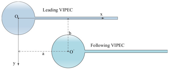
Figure 1.
The design parameters of a Vortex Induced Piezoelectric Energy Converter (VIPEC) farm, where O is the origin of coordinate as well as the center of the leading cylinder and is the center of the following cylinder.
CFD simulations were conducted with various groups of design parameters () with a changing from 0 to 6 in an interval of 1 and b changing from 0 to 4.5 in an interval of 0.75. It should be mentioned that layout parameters that induce geometry interference were not simulated.
3. CFD Method
The CFD simulation process was implemented using the commercial code ANSYS 15.0, which has established excellent credibility in the engineering field.
3.1. Computational Domain and Boundary Conditions
For the sake of calculation accuracy, the computational domain was extended ahead 15 D from the center of the leading VIPEC’s cylinder and extended backwards for 25 D from the center of the following one. Each VIPEC’s center was 10 D away from its nearest side wall. Thus, the whole computational domain had a size of (40 + a) (20 + b) D, which is large enough to eliminate the influence of walls on the flow field [17].
Since the VIPEC was scheduled to work in an underwater environment, its governing equation was the incompressible Navier–Stokes equation, and its voltage performance was evaluated with Equation (1). Periodical vortex shedding occurred at the back of the cylinder and detached from either side of it due to the flow separation around the cylinder. Studies on a single VIPEC including its governing equations, boundary conditions, the influence of geometric parameters on its hydrodynamic, and voltage performance have been elaborated in previous work [15]. Therefore, this paper puts emphasis on the interaction of two VIPECs and tries to determine their optimal layout parameter.
A steady and uniform velocity inlet boundary was adopted in the left wall of the domain, and the inlet flow velocity was set to be 2.6 m/s. A pressure outlet boundary was chosen for the right wall of the domain and smooth wall conditions were imposed at two side walls of the domain. Due to the narrow gap between the cylinder and the internal revolute joint inside it, the plate was solely stuck with piezo patches rather than the cylinder. As a result, the plate’s vibration amplitude was bounded and it was possible to approximate the output voltage with a stationary VIPEC with high precision through a two-dimensional simulation, as explained in previous work [15]. Hence, stationary wall conditions were implemented on all sides of the VIPEC including the cylinder and the plate, i.e., both the zero normal and tangential velocity conditions were imposed on those walls. The output voltage was predicted at the plate’s average position like a single VIPEC to evaluate its performance [15].
3.2. Mesh Generation and Independence Validation
The clustering of mesh elements in the zone of interest is a common practice as it reduces the computational cost while properly resolving the important features of the flow. Since shedding vortices march downwards behind the VIPEC, a local zone was refined with higher resolution grids (as shown in Figure 2). A boundary layer is added around the VIPEC to capture the complex boundary flow and flow separation. In order to obtain more accurate results with as few cells as possible, a grid independence validation was conducted with three different cell numbers. The cell number was mainly controlled by the maximum face size in the refined zone. The validation results are listed in Table 1.
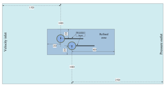
Figure 2.
Computational zone and boundary conditions.

Table 1.
Mesh resolution verification, where is RMS (Root Mean Square) of the lift coefficient on the cylinder, is RMS of the lift coefficient on the plate
As can be found in Table 1, mesh resolution changes from “coarse” to “medium”, hydrodynamic si mulation results, for the lift coefficient on the cylinder and for that on the plate, are markedly raised (by 27.0% for and 31.8% for ) with a relatively small increase in node number (12.6%). However, when mesh resolution varies from “medium” to “fine”, the node number increases dramatically (by 59.1%), while the simulation results don’t vary too much (by 4.1% for and 4.0% for ). Hence, medium mesh resolution is chosen in subsequent CFD simulation.
3.3. Timestep Setup
Choosing an appropriate time step () is essential to gather accurate simulation results in the shortest possible time. A time step verification with four different time step sizes was conducted to choose the most appropriate time step. The variations of instantaneous and its RMS (Root Mean Square) and frequency at four different time steps are drawn separately in Figure 3a,b.
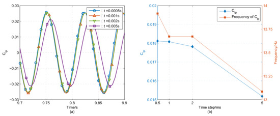
Figure 3.
Variations of (a) instantaneous (b) its RMS and frequency at four different time steps.
It can be noted from Figure 3a that the hydrodynamic simulation result, exemplified by , is affected by the time step size (). By marking = 0.0005 s as a benchmark, as exposed in Figure 3b, the RMS of and its frequency decrease by 0.21% and 1.75%, respectively, when it gets doubled, and by 1.64% and 1.75% when it gets quadrupled. However, when it increases to 0.005 s, they reduce dramatically by 16.21% and 5.96%. When the time consumption as well as the simulation accuracy is taken into consideration, = 0.002 s is chosen as the default time step in succedent studies.
4. Optimal Design Method
4.1. Kriging Surrogate Model
The Kriging surrogate model is an unbiased estimated model with the minimum variance. Generally, the predicted response is expressed () as [18]
with and , where p denotes the number of the basis function of the regression model. is the estimated response at sampled points, indicates the linear regression part, and is an n-dimensional vector representing n design variables (in this paper, for two layout parameters: the longitudinal spacing a and latitudinal spacing b). is the regression coefficient vector, and z(X) is the local deviation representing a Gaussian stationary stochastic process with the following statistical properties:
where m denotes the number of experiments (sampled points), is the variance of the stationary stochastic process, and is the stochastic-process correlation between two known points for which the Gaussian correlation function is usually adopted and can be written as
where is the k-th element of the correlation vector parameter , and is the kth element of points and . It can be used to expand to a correlation matrix between m sampled points: .
The resulting output from the function to be modeled based on m sampled points is written as
The correlation between an untried prediction point () and the m known sampled points is defined as follows:
Thus, for an untried design point, the best linear unbiased prediction of the response is
The final Kriging predictor, , is obtained ith [19]:
where is a vector including the value of evaluated at each of the sampled points, and is a m-dimensional vector composed of estimated response values at m sample points. is the least-squares estimated of and can be estimated as
The corresponding response surface model based on Kriging surrogate model was built as an optimization function using Matlab.
4.2. Particle Swarm Optimization
Particle swarm optimization (PSO) is a meta-heuristic algorithm that was developed in 1995 by Kennedy and Eberhart [20] and was first designed for simulating bird predatory behavior. It has been widely studied and applied in many fields since it was proposed [21,22,23]. A massless particle is designed to simulate a bird and the particle has two properties: velocity and position, which represent the speed and direction of movement respectively. The estimated value calculated from the established surrogate model is called the fitness value. Each particle searches for its optimal solution individually according the fitness value and records it as its personal best solution () and shares it to the entire group. The current group best solution is marked as . All the particles adjust their speeds and positions according to .
The steps of PSO are as follows:
- (1)
- Initialize N particles in the design space.
- (2)
- Calculate the fitness value (which represents the estimated values of the objective function at an desired point) for each particle according to a certain known model (f) which was derived from Kriging surrogate model in this paper.
- (3)
- Find each particle’s best fitness value in history and set its relevant position as the particle’s personal best solution ().
- (4)
- Compare the fitness values of all particles’ best solutions (s) and choose the overall best solution from all particles as their current global best solution ().
- (5)
- Update each particle’s velocity and position according to present information aswhere and are the particle velocity and position, the subscript i denotes the i-th component of the corresponding vector, t is the time, is the inertia factor, and are acceleration coefficients which represent the mean stiffness of the springs pulling a particle and are located between 0 and 4. In practice, the values of are almost ubiquitously adopted in PSO research [24].
- (6)
- The optimization process stops when the maximum number of iterations or minimum error criteria is achieved.
The general procedure of PSO is shown in Figure 4.
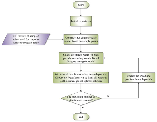
Figure 4.
The generalized procedure of particle swarm optimization (PSO).
5. Results and Discussion
5.1. Sampled Points Distribution
The layout configuration of two VIPECs can be divided into four parts according to the relative position of the leading/following VIPEC (i.e., a and b): the interference region, the tandem region, the parallel region, and the staggered region. Each region has its own characteristics due to the interaction of the leading/following VIPEC’s flow field. The distribution of sampled points is depicted in Figure 5.
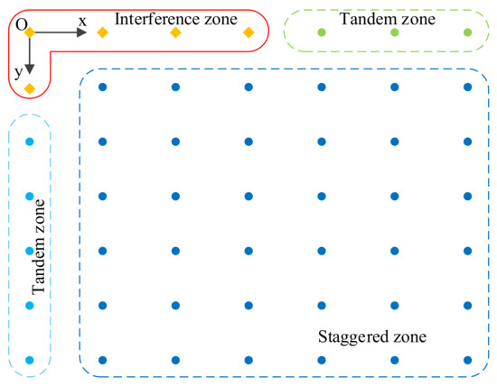
Figure 5.
Distributions of sampled points in the layout parameter design space used for the Computational Fluid Dynamics (CFD) simulation (♦ denotes a sampled point located in the interference region).
The layout parameter design space was bounded to : [0 D, 6 D] × [0 D, 4.5 D] according to the wake structure of a single VIPEC. Then, sample points were distributed by a varying from 0 to 6 in an interval of 1, and b varying from 0 to 4.5 in an interval of 0.75. It should be mentioned that five sampled points located in the interference region were not simulated due to the geometric interference of two VIPECs. Hence, a total number of 44 CFD simulation cases was conducted at these sampled points.
5.2. Instantaneous Hydrodynamic Performance of VIPECs in Four Different Regions
5.2.1. Nondimensionalized Lift Ratio
In order to investigate the influence of different layout configurations on the hydrodynamic performance of two VIPECs, i.e., the lift coefficients of two VIPECs’ plates, and , both of these lift coefficients were expressed as a nondimensional lift ratio by dividing of a single VIPEC (0.018075 in Table 1):
5.2.2. Interference Region
In the interference region, the layout configuration was unrealistic owing to the leading VIPEC interferring with the following one. Therefore, no CFD simulation was performed in this region.
5.2.3. Tandem Region
The tandem region means that the leading VIPEC and the following VIPEC are placed in tandem. The contours of pressure coefficient and velocity around two VIPECs at four different sampled points in the tandem region are presented in Figure 6. In this region, when the following VIPEC is located relatively close to the leading one, it will be surrounded by its leader’s wake. Thus, the follower’s high pressure region, which usually occurs at its front, is disturbed by its leader’s wake field. The disturbance can last for a rather long distance since the wake field exists for a long distance. This is, in fact, equivalent to the follower’s “inlet” flow no longer being a steady uniform free stream as a result of the leading VIPEC.
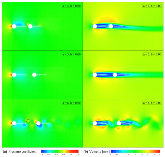
Figure 6.
Snapshots of contours of (a) the pressure coefficient and (b) the velocity around two Vortex Induced Piezoelectric Energy Converters (VIPECs) at three different tandem region sampled points.
It can be found from Figure 6 that at a = 4, b = 0.00, the stagnation point slipped along the cylinder obviously. This contributed to the low pressure area at one side of the leading plate not being able to conquer the high pressure existing at the front of the following VIPEC. Thus, it moved across the centerline and the stagnation point moved in the opposite direction. As the longitudinal spacing (a) increased, the influence of the following VIPEC’s high pressure zone on the leading plate’s end was impaired. At a = 5, b = 0.00, the low pressure was able to conquer the high pressure area and passed by the follower’s head laterally. However, owing to the VIPEC’s outer contour, the low pressure area wa mixed in this case, making the leader and follower a streamlined structure (as “a = 5, b = 0.00” shown in Figure 6). Thus, the lift forces on both plates were consequently severely inhibited.
At a = 6, b = 0.00, the impairment was further aggravated, and the follower’s high pressure area expanded and was forced to slip around the cylinder again (as shown in Figure 7). The flow separation points also experienced a shift forward due to the shift of the stagnation point which brought about a great decrease of . On the contrary, the shift of the follower’s high pressure area somewhat recovered the pressure field around the leader’s ipsilateral end (as the dashed area shown in Figure 6a “a = 6, b = 0.00”), and as a result, was slightly augmented.
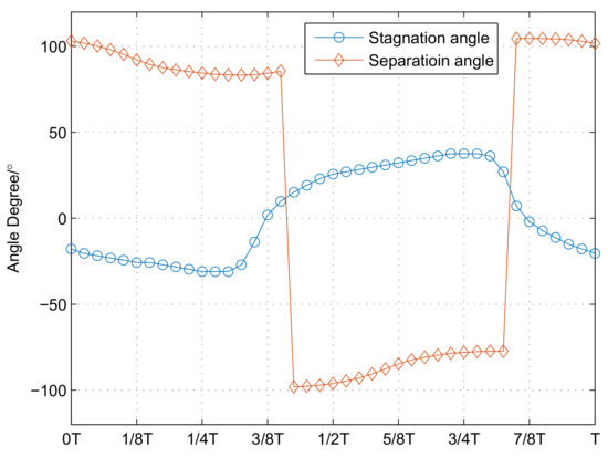
Figure 7.
The variation in the stagnation and separation angles for a = 6, b = 0.00 during a single period.
5.2.4. Parallel Region
The parallel region is located at . In this region, the flow between the leading and following VIPEC behaves like a pipe flow, and the contours of nondimensional vorticity and velocity around the two parallel VIPECs are shown in Figure 8.
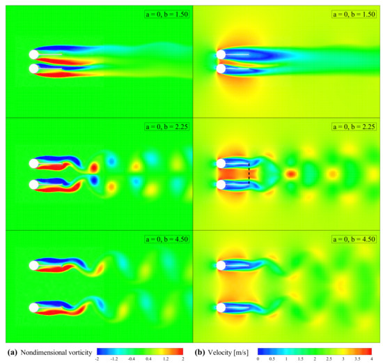
Figure 8.
Snapshots of contours of (a) nondimensional vorticity and (b) velocity at three different sampled points in the parallel region.
Figure 8 reveals that at a = 0, b = 1.50, an alternating lift force was not produced due to the mutual interference of the pressure field in the narrow spacing between two plates. With an increase in the latitudinal spacing (b), the flow between two VIPECs was apparently accelerated and it induced an extensive low pressure area with an enlarged amplitude around the inner side of VIPECs (Figure 8 “a = 0, b = 2.25”). This can be explained by Bernoulli’s theorem—the high velocity corresponds to a small pressure. When fluid flows through the intermediate zone between VIPECs, the flow is accelerated and corresponding pressure decreases. Thus, a smaller b produces a broader low pressure area with a greater negative amplitude. When b is large enough, the interaction of the relative high pressure disappears (as shown in Figure 8a “a = 0, b = 4.50”). What is more, it’s worth mentioning that the wake structure of two VIPECs remained in the 2S pattern (a single vortex shed from each side of the cylinder in half a period) which is similar to that of a single VIPEC.
The variations of and for a = 0, b = 2.25 are illustrated in Figure 9. Their phase difference remained at due to the similar level of low pressure between the two VIPECs’ intermediate gap; however, on the plates’ opposite sides, the amplitude was also approximately equal due to the symmetry of the flow. The velocity profile on the outlet of the virtual pipe between two VIPECs, i.e., the connecting line of two plates’ tips (the black dashed line shown in Figure 8b “a = 0, b = 2.25”) depicted in Figure 10, had the typical characteristics of pipe flow. That is, the velocity profile was symmetrical, and the velocity was lowest at both ends and increased along the radial direction.
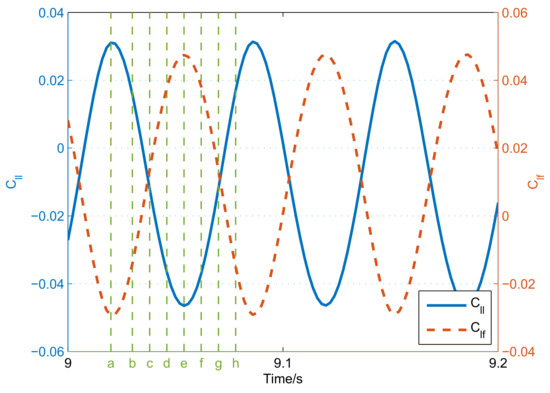
Figure 9.
Curves of instantaneous lift coefficients of the leading and following VIPECs at a = 0, b = 2.25.
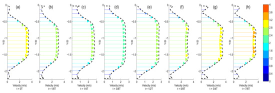
Figure 10.
Transient velocity profiles of the virtual pipe’s outlet (the inner connecting line of two VIPECs’ tips) during a period.
5.2.5. Staggered Region
The staggered region is located where a as well as b. The influence of different layout configurations on the plates’ lift force is marked in Figure 11. In this region, the effect of various layout configurations on , and can be divided into six types: (1) , , both enhanced, (as “a = 5, b = 0.75” shown in Figure 12); (2) , enhanced, inhibited, (as “a = 2, b = 1.50” shown in Figure 12); (3) , enhanced, inhibited, (as “a = 3, b = 3.75” shown in Figure 12); (4) , , both inhibited, (do not exist in the staggered region; however, they do exist in the tandem region, as “a = 5, b = 0” shown in Figure 6); (5) , inhibited, enhanced, (as “a = 6, b = 4.50” and “a = 2, b = 3.00” shown in Figure 13); (6) , inhibited, enhanced, (as “a = 1, b = 0.75” shown in Figure 13). It can be observed from Figure 11 that was enhanced when the follower VIPEC was close to the leading one and inhibited when their spacing increased, while the change of was the opposite.
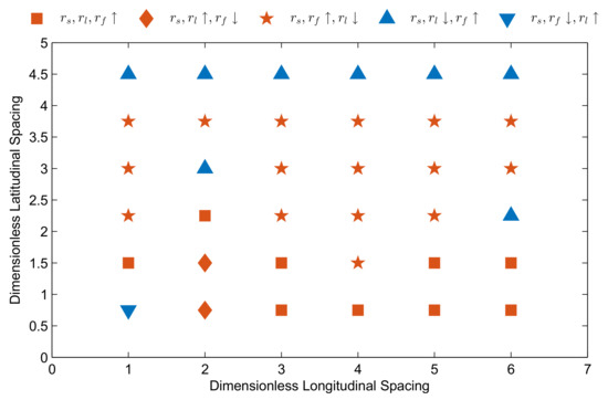
Figure 11.
The marked enhancement/inhibition of , , and at various sampled points in the staggered region.
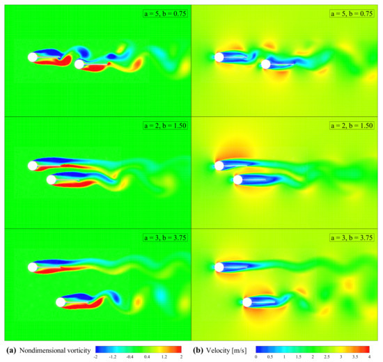
Figure 12.
Snapshots of contours of (a) nondimensional vorticity and (b) velocity around two VIPECs at three different enhanced sampled points in the staggered region.
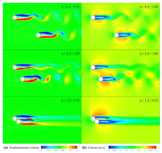
Figure 13.
Snapshots of contours of (a) nondimensional vorticity and (b) velocity around two VIPECs at two different inhibited sampled points in the staggered region.
It can be noted from Figure 11 that was pervasively enhanced in the simulated staggered zone. However, the enhancement resulted from various reasons. The contours of nondimensionalized vorticity and velocity around two VIPECs with an enhanced for three different layout configurations are shown in Figure 12.
For the sampled points where was enhanced (such as a = 5, b = 0.75 and a = 2, b = 1.50 in Figure 12, the following VIPEC was located in the neighborhood of the leader’s plate, and then the front high pressure area was able to act on the leader’s plate directly; thus, a greater amount of pressure was produced over its two sides. However, its wake structure was strongly destroyed since it was difficult to conquer the increased adverse pressure gradient in the leading cylinder’s lower side. Hence, the lift coefficient became larger while quasi-stable. The pervasive enhancement of (such as a = 2, b = 1.50 and in Figure 12) contributed to the leader’s lateral high velocity. With a higher inlet velocity and less disturbance from its wake, had different degrees of increase according to the relative spacings. What is more, when the two VIPECs were close enough (say, a = 2, b = 1.50 in Figure 12), both VIPECs’ wakes were destroyed due to their interaction. Periodical vortex shedding no longer existed and both the lift force and the wake field tended to be stable.
Figure 11 shows that sampled points with inhibited were generally located at the boundaries of the simulated staggered zone. The contours of nondimensionalized vorticity and velocity around two VIPECs with an inhibited for three different layout configurations are shown Figure 13.
With the increase in the longitudinal and latitudinal spacings, the mutual interference between two VIPECs tended to be slender; thus, was almost unaffected, though showed a slight decrease (a = 6, b = 4.50 in Figure 13). Generally, the enhancement/inhibition of was determined by whether the increase of could compensate for the decrease of . For the sampled point a = 2, b = 3.00 in Figure 13, decreased by 89.51%, while increased by 52.00%, and then a inhibition of was produced. However, an increase of and a decrease of occurred at a = 1, b = 0.75, as shown in Figure 13 due to the very close spacing between two VIPECs. Meanwhile, the lift force tended to be quasi-stable and the flow tended to be steady which is similar to that of a = 2, b = 0.75 in Figure 12.
5.3. Output Voltage Performance
The open circuit output voltage was also nondimensionalized by dividing the (1.2880 mV calculated from a single VIPEC) of a single VIPEC:
It is worth mentioning that the output voltage was not consistently proportional to the amplitude of the generated lift force. In several specified configurations, the lift force remained at a relative high level since the pressure difference over the plate remaiend high and unchanged, such as “a = 5, b = 0.00” in Figure 6, a = 0, b = 1.50 in Figure 8, a = 2, b = 1.50 in Figure 12 and a = 1, b = 0.75 in Figure 13. These layout configurations were concentrated at locations where the following VIPEC was located at the very vicinity of the leading one. This was because the flow tended to be steady after passing through the narrow gap. Meanwhile, the inner side of the leading plate was always in a high pressure area due to the compensation of the following VIPEC which resulted in a quite constant big force. However, alternative force rather than constant force induces output voltage. Negligible voltage was generated in these cases as a consequence.
6. Kriging Surrogate Model and PSO Optimization
The CFD simulation results for various VIPEC layout configurations are listed in Table 2. Based on these results, the response surface model was established with the Kriging surrogate model in the simulated parameter space.
Table 2.
Simulation results for different layout configurations.
6.1. Response Surface Model for the Output Voltage
6.1.1. Response Surface Model for the Leading VIPEC’s Output Voltage
The influence of different layout configurations on the leading VIPEC’s voltage performance was revealed by the response surface model of , established through the Kriging surrogate model, which is illustrated in Figure 14.
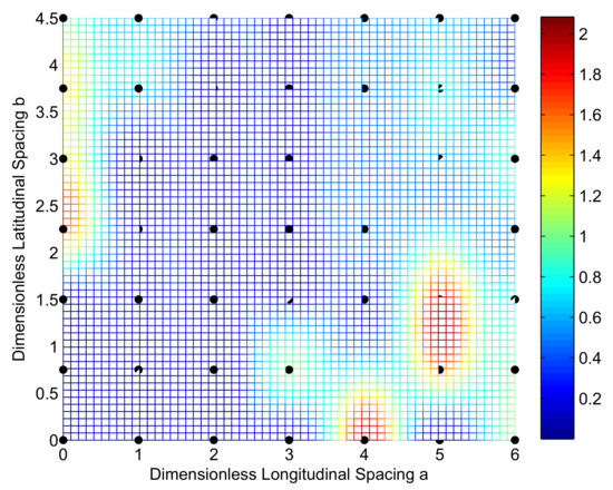
Figure 14.
Kriging response surface model for .
It can be deduced from Figure 14 that the enhanced zone on was mainly concentrated in two locations. The first one was in the parallel region around a = 0, b = 1.5–3, and this was mainly caused by the flow velocity incrementation as it passed between the plates (as shown in Figure 6). The second one was around a = 5, b = 1.50. In this area, the follower’s cylinder lagged behind the leader’s plate, which resulted in the high pressure at its front acting on the leader’s plate directly (Figure 12). Then, was reinforced and a larger was generated. However, outside the enhanced zone, was pervasively inhibited below 1 and this was essentially caused by the destruction of the leader’s wake field due to the presence of the follower (for example, “a = 2, b = 1.50” in Figure 12). Meanwhile, this indicates that when the following VIPEC was located far from the leading one, the pressure on one side of the leading plate only received slight compensation from the following VIPEC’s front-located high pressure region, which was exemplified by the variation in as a = 5, b = 0.75 shown in Figure 12.
6.1.2. Response Surface Model for the Following VIPEC’s Output Voltage
The influence of the layout configuration on was also investigated with the surrogate model. The response surface model established through the Kriging surrogate model is illustrated in Figure 15.
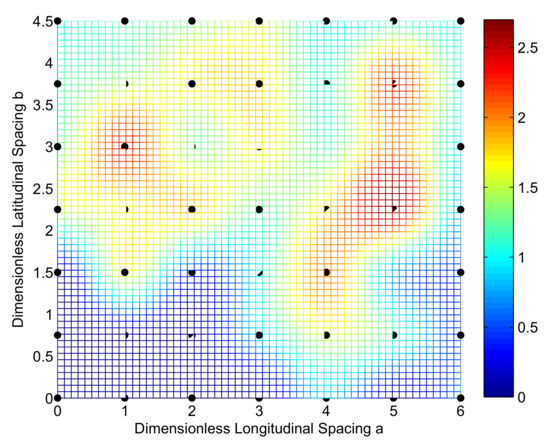
Figure 15.
Kriging response surface model for .
Figure 15 reveals that the layout’s influence zone of tended to be opposite to that of . The inhibited zone of was the dominating neighborhood of the following VIPEC as : [0, 2.7] × [0, 1.5]. This was also due to the following VIPEC being located in the very neighborhood of the leading plate, causing the flow between their gap to be steady, and thus large but stable , were generated (Figure 12). Another extremely inhibited zone was locates where two VIPECs are in the tandem region, especially when the following VIPEC located in the leading one’s wake and formed a streamline shape as a = 5, b = 0.00, shown in Figure 6. The lift force on the follower’s plate was close to 0 in this case. Beyond the inhibited zone, was pervasively enhanced, even doubled, which resulted from the accelerated flow between two VIPECs contributing to an increase in the pressure difference on both sides of the follower’s plate.
6.1.3. Response Surface Model for Two VIPECs
The summation of two VIPECs’ output voltages is the most important variable to obtain a better overall performance. Hence, the Kriging response surface model of the total output voltage () was established. Then, PSO optimization was conducted over the obtained model to search for the optimal layout parameters. The established response surface model is shown in Figure 16.
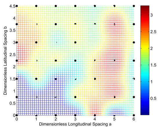
Figure 16.
Kriging response surface model for .
Figure 16 reveals that the enhanced zone of was also mainly divided into two parts. The first one was located in the parallel region around a = 0, b = 1.5–3, which is in accordance with that of and can be explained with the same reasoning. However, the parallel layout optimization is often infeasible in practical applications due to its instability. The second part covered a broader zone around : [4.3, 5.5] × [0.5, 5.2]. This extension, compared to that of , mainly contributed to a larger in this zone.
6.2. Comparisons of the Optimal Layout between CFD and PSO
The optimal layout parameters found through PSO on the response surface model of were a = 4.9377, b = 2.2483, as shown in Table 3. The optimization result was verified through the comparison of the predicted results and the CFD simulation. It can be found from Table 3 that the relative error between the predicted and that obtained from CFD simulation was 3.8% which proves that the combined Kriging surrogate model and PSO can give a good prediction of the VIPECs’ overall performance.
Table 3.
The comparison of the predicted and CFD simulation (the summation of two VIPECs’ output voltage ratios) results with the optimal layout parameters.
The time-varying lift force, output voltage, and a snapshot of contours of the transient pressure coefficient at different moments during a period are presented in Figure 17.
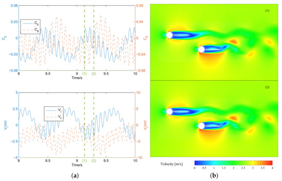
Figure 17.
(a) Time-varying lift force and output voltage and (b) snapshots of velocity contours during a period with optimal layout parameters.
The optimal layout configuration reached a balance between two VIPECs. Though the amplitude of the leading VIPEC’s lift force was slightly impaired, that of the following one was firmly enhanced. Then, an enhancement to the summation of both lift forces () was produced. Besides, it can be inferred from Figure 17 that with this layout, the variation in and was more sensitive, which is beneficial for the alternative output voltage. Under these combined actions, the open circuit output voltage () increased. The predicted result agreed with that of CFD simulation, as shown in Table 3, which indicates that the Kriging surrogate model combined with the Particle Swarm Optimization method can be used for the layout optimization of two VIPECs.
7. Conclusions
The layout configuration of two VIPECs is characterized by two dimensionless parameters: the nondimensionalized longitudinal spacing (a) and the nondimensionalized latitudinal spacing (b), which are invoked as design parameters. A computational fluid dynamics simulation for various layout parameters was carried out. The lift force was obtained from the CFD simulation results. Then, a generated open circuit voltage is computed using the established equation. The influence of the layout parameters on the plate’s lift force and wake structure was elaborated. Response surface models for the leading/following VIPEC’s open circuit output voltage and their summation were established using the Kriging surrogate model. Optimal design parameters were acquired through Particle Swarm Optimization, and the predicted result agreed well with the CFD simulation. The main conclusions of this study are as follows:
- When placed in tandem, the follower’s lift force is greatly inhibited, since its inlet flow is disturbed by the leading VIPEC which is reflected directly through the periodic shifts of the stagnation and separation angles, while it is enhanced by the extensive low pressure area inside the two VIPECs, which is induced by the velocity acceleration of the pipe-like flow between the leader and follower’s plates.
- The CFD results showed that the lift force on the leading/following VIPEC is determined by the layout parameters when they are staggered. The area of influence on the leader’s lift force is mainly situated where the follower is located in the vicinity of the leader’s plate. However, the follower’s lift force is pervasively enhanced except when it is located in the very neighborhood of the leader’s plate, and this mainly contributes to the leader’s high lateral velocity which serves as its income velocity.
- The influence of layout parameters on the open circuit output voltage is not consistent with that of the lift force, since the output voltage is induced by alternative force. When the following VIPEC is located too close to the leading one, their wake fields are destroyed, and their lift forces tend to be large but quasi-stable, and the output voltage is consequently negligible.
- The optimal layout parameters for the summation of the output voltage are a = 4.9377, b = 2.2483, and the total output voltage is predicted to increase by 63.7% compared to that of two single VIPECs. The predicted result agrees well with that gathered by the CFD simulation.
Author Contributions
X.A. conceived the study and performed the CFD simulations; X.A., B.S. and Z.M. analyzed the simulation results; X.A. wrote the manuscript; Z.M. and C.M. reviewed and edited the manuscript.
Funding
This research was supported by the National Natural Science Foundation of China (Grant No. 61572404).
Conflicts of Interest
The authors declare no conflict of interest.
Nomenclature
| D | Cylinder’s diameter |
| Two VIPECs’ longitudinal distances | |
| Two VIPECs’ latitudinal distances | |
| A single VIPEC’s lift coefficient | |
| Leading VIPEC’s lift coefficient | |
| Following VIPEC’s lift coefficient | |
| A single VIPEC’s output voltage | |
| Leading VIPEC’s output voltage | |
| Following VIPEC’s output voltage | |
| L | Plate’s length |
| Dimensionless longitudinal distance | |
| Dimensionless latitudinal distance | |
| Leading VIPEC’s lift coefficient ratio | |
| Following VIPEC’s lift coefficient ratio | |
| Summation of two VIPECs’ lift coefficient ratios | |
| Leading VIPEC’s output voltage ratio | |
| Following VIPEC’s output voltage ratio | |
| Summation of two VIPECs’ output voltage ratios |
References
- Bernitsas, M.M.; Raghavan, K.; Ben-Simon, Y.; Garcia, E.M.H. VIVACE (Vortex Induced Vibration for Aquatic Clean Energy): A New Concept in Generation of Clean and Renewable Energy from Fluid Flow. J. Offshore Mech. Arct. Eng. 2008, 130, 619–636. [Google Scholar] [CrossRef]
- Bernitsas, M.M.; Ben-Simon, Y.; Raghavan, K.; Garcia, E.M.H. The VIVACE Converter: Model Tests at High Damping and Reynolds Number Around 105. Offshore Mech. Arct. Eng. 2009, 131, 403–414. [Google Scholar] [CrossRef]
- Akaydin, H.D.; Elvin, N.; Andreopoulos, Y. Wake of a cylinder: A paradigm for energy harvesting with piezoelectric materials. Exp. Fluids 2010, 49, 291–304. [Google Scholar] [CrossRef]
- Akaydin, H.D.; Elvin, N.; Andreopoulos, Y. The performance of a self-excited fluidic energy harvester. Smart Mater. Struct. 2012, 21, 25007–25019. [Google Scholar] [CrossRef]
- Vinod, A.; Kashyap, A.; Banerjee, A.; Kimball, J. Augmenting Energy Extraction from Vortex Induced Vibration Using Strips of Roughness/Thickness Combinations. In Proceedings of the Marine Energy Technology Symposium, Washington, DC, USA, 15–17 April 2013. [Google Scholar]
- An, X.; Song, B.; Mao, Z.; Ma, C. The mathematical modeling of a novel anchor based on vortex induced vibration. In Proceedings of the OCEANS, Shanghai, China, 10–13 April 2016; pp. 1–5. [Google Scholar] [CrossRef]
- An, X.; Song, B.; Tian, W.; Ma, C. Numerical simulation of Vortex Induced Piezoelectric Energy Converter (VIPEC) based on coupled fluid, structure and piezoelectric interaction. In Proceedings of the OCEANS 2017-Aberdeen, Aberdeen, UK, 19–22 June 2017; pp. 1–5. [Google Scholar]
- Box, G.E.; Draper, N.R. Response Surfaces, Mixtures, and Ridge Analyses; John Wiley & Sons: Hoboken, NJ, USA, 2007; Volume 649. [Google Scholar]
- Laurent, L.; Riche, R.L.; Soulier, B.; Boucard, P. An Overview of Gradient-Enhanced Metamodels with Applications. Arch. Comput. Methods Eng. 2017, 3, 1–46. [Google Scholar] [CrossRef]
- Majdisova, Z.; Skala, V. Radial basis function approximations: Comparison and applications. Appl. Math. Model. 2017, 51, 728–743. [Google Scholar] [CrossRef]
- Press, W.H. Numerical Recipes 3rd Edition: The Art of Scientific Computing; Cambridge University Press: Cambridge, UK, 2007. [Google Scholar]
- Zhang, B.; Teng, H.F.; Shi, Y.J. Layout optimization of satellite module using soft computing techniques. Appl. Soft Comput. 2008, 8, 507–521. [Google Scholar] [CrossRef]
- Biswas, P.P.; Suganthan, P.N.; Amaratunga, G.A.J. Decomposition based multi-objective evolutionary algorithm for windfarm layout optimization. Renew. Energy 2017, 115, 326–337. [Google Scholar] [CrossRef]
- Tian, W.; Mao, Z.; Zhao, F.; Zhao, Z. Layout Optimization of Two Autonomous Underwater Vehicles for Drag Reduction with a Combined CFD and Neural Network Method. Complexity 2017, 2017, 1–15. [Google Scholar] [CrossRef]
- An, X.; Song, B.; Tian, W.; Ma, C. Design and CFD Simulations of a Vortex-Induced Piezoelectric Energy Converter (VIPEC) for Underwater Environment. Energies 2018, 11, 330. [Google Scholar] [CrossRef]
- Dehez, B. Improved constitutive equations of piezoelectric monomorphs: Application to the preliminary study of an original traveling-wave peristaltic pump. Sens. Actuators A Phys. 2011, 169, 141–150. [Google Scholar] [CrossRef]
- Prasanth, T.K.; Mittal, S. Effect of blockage on free vibration of a circular cylinder at low Re. Int. J. Numer. Methods Fluids 2008, 58, 1063–1080. [Google Scholar] [CrossRef]
- Sakata, S.; Ashida, F.; Zako, M. On applying Kriging-based approximate optimization to inaccurate data. Comput. Methods Appl. Mech. Eng. 2007, 196, 2055–2069. [Google Scholar] [CrossRef]
- Kaymaz, I. Application of kriging method to structural reliability problems. Struct. Saf. 2005, 27, 133–151. [Google Scholar] [CrossRef]
- Kennedy, J.; Eberhart, R. Particle swarm optimization. In Proceedings of the IEEE International Conference on Neural Networks, Perth, Australia, 27 November–1 December 1995; Volume 4, pp. 1942–1948. [Google Scholar] [CrossRef]
- Bratton, D.; Blackwell, T. A simplified recombinant PSO. J. Artif. Evol. Appl. 2008, 2008, 14–23. [Google Scholar] [CrossRef]
- Roy, R.; Dehuri, S.; Cho, S.B. A novel particle swarm optimization algorithm for multi-objective combinatorial optimization problem. Int. J. Appl. Metaheuristic Comput. 2011, 2, 41–57. [Google Scholar] [CrossRef]
- Bonyadi, M.R.; Michalewicz, Z. Particle swarm optimization for single objective continuous space problems: A review. Evol. Comput. 2017, 25, 1–54. [Google Scholar] [CrossRef] [PubMed]
- Chen, H.N.; Zhu, Y.L.; Hu, K.Y.; Ku, T. Global optimization based on hierarchical coevolution model. In Proceedings of the 2008 IEEE Congress on Evolutionary Computation, Hong Kong, China, 1–6 June 2008; pp. 1497–1504. [Google Scholar]
© 2018 by the authors. Licensee MDPI, Basel, Switzerland. This article is an open access article distributed under the terms and conditions of the Creative Commons Attribution (CC BY) license (http://creativecommons.org/licenses/by/4.0/).