Lifetime Prediction of a Polymer Electrolyte Membrane Fuel Cell under Automotive Load Cycling Using a Physically-Based Catalyst Degradation Model

Abstract

One of the bottlenecks hindering the usage of polymer electrolyte membrane fuel cell technology in automotive applications is the highly load-sensitive degradation of the cell components. The cell failure cases reported in the literature show localized cell component degradation, mainly caused by flow-field dependent non-uniform distribution of reactants. The existing methodologies for diagnostics of localized cell failure are either invasive or require sophisticated and expensive apparatus. In this study, with the help of a multiscale simulation framework, a single polymer electrolyte membrane fuel cell (PEMFC) model is exposed to a standardized drive cycle provided by a system model of a fuel cell car. A 2D multiphysics model of the PEMFC is used to investigate catalyst degradation due to spatio-temporal variations in the fuel cell state variables under the highly transient load cycles. A three-step (extraction, oxidation, and dissolution) model of platinum loss in the cathode catalyst layer is used to investigate the cell performance degradation due to the consequent reduction in the electro-chemical active surface area (ECSA). By using a time-upscaling methodology, we present a comparative prediction of cell end-of-life (EOL) under different driving behavior of New European Driving Cycle (NEDC) and Worldwide Harmonized Light Vehicles Test Cycle (WLTC).

1. Introduction

Fuel cell durability is currently the biggest bottleneck in the commercialization of fuel cell electric vehicles. In a highly transient loading environment such as an automobile, a fuel cell does not only undergo potential cycling but also cycling of various internal state variables such as temperature, pressure and humidity. Such a cyclic operation leads to multiple degrading side reactions, eventually rendering the fuel cell unable to provide the requested power demand or fail catastrophically. One of the weak links with respect to the durability of fuel cell components is the catalyst layer (CL). The commonly used platinum (Pt)-based catalysts are state of the art due to their low overpotentials and high catalytic activities for hydrogen oxidation reaction (HOR) and oxidation reduction reactions (ORR) [1,2], but the downside is that they are expensive and prone to high rates of degradation. In order to predict fuel cell durability or propose effective mitigation strategies, one needs to focus on degradation mechanisms leading to Pt loss, including the search for lifetime-extending operating strategies.

Irreversible catalyst degradation occurs through various mechanisms such as Pt dissolution, particle growth by Ostwald ripening, coalescence of particles and detachment from the carbon support following carbon corrosion [3], but to add to the complexity of the catalyst degradation process, irreversible catalyst degradation has also been shown to be mitigated by a reversible degradation process such as Pt oxidation, which can protect the Pt from dissolution at potentials above 1.1 V [4]. Nevertheless, any kind of catalyst degradation eventually leads to a loss of electrochemically active surface area (ECSA) or loss of catalyst contact with electron conductors (e.g., carbon support). Many researchers have explored the phenomena leading to Pt dissolution and corresponding ECSA loss in PEMFCs [5,6,7]. Zhang et al. reviewed the various plausible degradation mechanisms for Pt-based catalysts [8]. Bi et al. [9] explored the effect of humidity and oxygen concentration on Pt dissolution rates and found that a reduction in humidity reduces the rate of Pt dissolution while oxygen concentration has a quite insignificant contribution.

The inhomogeneity in the CL due to manufacturing defects and the load-based spatial distribution of reactant concentration and pressure gradients in the flow field also leads to a spatially varying cell operating behavior. The spatial inhomogeneity of a catalyst layer has been studied by Bussian et al. [10] using atomic force microscopy. This in turn causes spatial gradients in the electrochemical properties of the fuel cell components and consequently creates specific areas of variable performance in the membrane electrode assembly (MEA), which results in the non-homogenous distribution of the local current density [11,12]. Most single cell or system level cell performance evaluations only provide a spatially averaged insight into cell voltage and current values that does not reveal the spatial resolved behavior of the cell state variables. Since the reported cell failure cases in the literature show highly localized cell component degradation [13], a spatially averaged analysis will not be able to provide a thorough insight into the causes of the cell failure and to propose appropriate mitigation strategies.

One of the interesting methodologies to study spatially resolved local cell behavior is to use a segmented cell system [14,15,16]. However, the invasive segmented cell studies influence the cell operation and are limited by cell and component geometries. The non-invasive techniques involve complicated and expensive diagnostic tools [17,18]. Hence, in order to understand the locally resolved cell behavior, there is a concrete need for more flexible and economic non-invasive techniques.

Further, the rate of Pt dissolution is also greatly influenced by the nature of cell loading. Uchimura et al. [19] studied the effect of various potential cycle profiles on the Pt dissolution rates. They measured the changes in ORR specific activity due to the loss ECSA through cyclic voltammetry. However, the effect of a realistic load cycle on ECSA loss is still not investigated. In order to come up with an effective degradation mitigation (or durability enhancement) strategies, fuel cell durability should be evaluated under realistic load cycling. Although there have been some studies on the long term durability and performance of a fuel cell in a transportation based load cycle [20,21], performing parametric studies on experimental test benches that run for highly extended periods viz. hundreds of hours, is not practical.

Multiphysics modeling of fuel cell transport process and electrochemistry and their interaction with cell geometry, operating conditions, degradation mechanisms, and load cycles, assist in understanding the complex coupling between cell components and underlying physical phenomena. They also help optimizing the parameter space for experimental investigation, thus economizing time and money. There have been multiple attempts to model component degradation [20,21,22,23,24] in PEMFCs but application of those degradation mechanisms towards estimation of PEMFC durability is still missing in the existing literature. Mayur et al. [25] developed a multiscale approach for on-the-fly coupling between a car model (system-scale), 2D single fuel cell model (cell-scale), and degradation model (nanoscale). A piecewise linear time upscaling methodology was developed to achieve end-of-life (EOL) predictions for the fuel cell in operation for a faster prediction of cell durability and performance reduction with respect to the cell state variables.

This paper focuses on the role of different automobile induced load cycles on Pt dissolution and its effect on durability of a PEMFC. The catalyst degradation model that is used in this work relies on a mechanistic approach at the nanoscale and only considers Pt dissolution as a degradation mechanism developed by Robin, Gerard et al. [26,27]. With the help of a 2D transport model of a PEMFC developed by Bao et al. [28], the spatially resolved cell performance and durability is discussed with respect to Pt dissolution and the ensuing reduction in ORR activity due to ECSA loss. The time upscaling methodology and virtual fuel cell car model of Mayur et al. [25] is used for durability predictions under two separate driving cycle (DC) loads, namely, New European Driving Cycle (NEDC) [29] and Worldwide Harmonized Light Vehicles Test Cycle (WLTC) [30].

2. Simulation Methodology

2.1. Overview of Simulation Framework

The simulation framework used in this study has been presented previously [25] and is only summarized here. Figure 1 shows the multiscale coupling of models where a two-way approach (bottom-up and top-down) is used to predict durability of fuel cells in an automobile application. In this methodology, the top-down direction starts from the system-generated transient load conditions for the fuel cell, which causes a transient variation in the state variables of the cell. The bottom-up direction starts from the degradation library (which is based on nanoscale studies). The generated degradation rates follow the transient changes in the fuel cell state variables and lead to a component-level performance loss of the fuel cell. The two-way approach leads to an active integration of the system model (fuel cell car) and component model (single cell) extended onto microscopic physicochemical processes governing degradation mechanisms. Firstly, the system model (Simulink) generates highly dynamic power demand ($P_{\mathrm{d},\mathrm{cell}}$) by matching the velocity requirement of the driving cycle ($u_{\mathrm{d}}\left(t_{\mathrm{DC}}\right)$) to the fuel cell power demand. The power is supplied by a fuel cell stack that is modeled by upscaling the single-cell generated power supply. The fuel cell model (COMSOL) interacts on the fly with the degradation library that provides instantaneous degradation factor ($f_{\mathrm{deg},\mathrm{C}}$) based on included degradation mechanisms through look-up tables (LUT), analytical functions or empirical mappings. The Simulink model simulates the time duration of a single driving cycle ($t_{\mathrm{DC}}$). The total degradation over the driving cycle is calculated in MATLAB (2016a), which linearily upscales the degradation over one driving cycle to over ‘n’ driving cycles. This new state of degradation via the upscaled degradation factor ($f_{\mathrm{deg},\mathrm{C}}^{\mathrm{up}}$) is set into the COMSOL model via Simulink. The entire framework is controlled in MATLAB that runs the durability loop until the cell end-of-life ($t_{\mathrm{EOL}}$). The details of the various components shown are discussed in the following sections.

2.2. Fuel Cell Car Model

The fuel cell car model is a modular representation of various components of a mid-size car that has an automotive driving cycle as an input and converts it into a cell-level power demand, as described in detail in our previous work [25].

Table 1. Parameters for the fuel cell car and fuel cell stack.

Parameter	Value
Mass of car + H2 tank (m)	1100 kg + 99.7 kg a
Coefficient of rolling resistance (Cr)	0.0085 a
Drag coefficient (Cw)	0.3 a
Shadow area (A)	1.91 m2 a
Final drive ratio (ηgear)	6.066 a
Powertrain efficiency (ηPT)	0.8 a
Wheel radius (Rw)	0.291 m a
Auxiliary power consumption	400 W a
Fuel cell stack power	75 kW c
Number of cells in the stack (Nstack)	315 b
Active cell area	0.025 m2
Total stack weight	153.8 kg b
Stack power density	0.49 kW/kg c
Proportional gain (Kp)	5 c
Integrator gain (KI)	0.6 c

^a Estimated from a middle-size passenger car. ^b Taken from Auto-Stack project [31]. ^c Tuned parameters.

shows the car and stack parameters used in the current study. Figure 2 shows the velocity variation and corresponding predicted stack power demand from the driving cycles, NEDC and WLTC.

Table 2. Characteristics of the driving cycle load.

Characteristics	NEDC	WLTC
Duration	1180 s	1800 s
Idling duration	280 s	242 s
Theoretical distance	11,023 m	23,262 m
Maximum speed	120 km/h	131.3 km/h
Maximum stack power	37.9 kW	44.9 kW

lists some basic characteristics of the two driving cycles.

2.3. Single Cell Model

The single cell model is based on a 2D transport model where the electrochemistry is described with a modified Butler-Volmer equation derived from elementary kinetics mechanisms, as published previously [25,28]. The transport properties of the porous gas diffusion layer (GDL) and the polymer electrolyte membrane (PEM) are taken to be isotropic. The thickness of the catalyst layer is not spatially resolved in this study and contributes as a boundary source/sink term for reaction products and reactants. It has been shown in the literature that catalyst layer structure and the Pt transport in catalyst layer (CL) give more detailed insights into the volume-specific electrochemistry and species transport, which affect the cell performance, specially in the case of low Pt loading conditions (ca. 0.025 mg/cm²) [32,33], but in this work, we decided to use a reduced complexity model with a uniform distribution of Pt (loading of 0.15 mg/cm²) along the CL. Further, we hypothesize that the Pt dissolution in the CL is significantly influenced by the local cell parameters such as cell voltage, oxygen, and water concentration, mainly originating from the transport in the GDL and the membrane. Consequently, the CL was approximated as a line source/sink of the species where the direct consequence of Pt dissolution was the loss in ECSA, as shown in the following sections. The reactant gases are assumed to be ideal and an isothermal model with single-phase transport for water is considered.

Figure 3 shows the cell geometry, which is a straight single channel with counter-flow configuration. The objective of the present work is to spatially resolve the cell performance and degradation under transient operation. To this goal, we investigate degradation at different positions along the continuous domain along the cathode catalyst layer (CCL) and the flow channels. Figure 3 shows the beginning ($y=0 \mathrm{m}$) and the end ($y=0.93 \mathrm{m}$) positions. For the cell operating conditions, we have assumed that the inlet pressure of cathode and anode channels is 250 kPa, at a temperature of 85 °C and a humidity of 100%. At such a high humidity, one shortcoming of the current model is that due to the single-phase treatment of water transport, the simulated partial pressure of water vapor can increase beyond its saturation partial pressure at high loads (which in the case of a two-phase water model would have been compensated by liquid water formation). This decreases the oxygen partial pressure in the model, thus influencing the effect of oxygen concentration in the Pt dissolution mechanism.

The cell is running in a lambda-controlled mode with cathode stoichiometry of 1.3 and anode stoichiometry of 1.5, so that fuel starvation does not occur. The lambda controlled inflow condition is calculated as shown in

Table 3. Parameter values for the Pt dissolution model from Robin et al. [26].

Parameters	Value
Pt dissolution rate constant, $k$	$2.2\times {10}^{-6} \mathrm{mol}/\left({\mathrm{m}}^2\mathrm{s}\right)$
Free energy for Pt extraction, $\Delta G_{\mathrm{s}}$	$75,000 \mathrm{J}$
Surface energy of Pt, ${\gamma }_{\mathrm{Pt}}$	$2.4 \mathrm{J}/{\mathrm{m}}^2$
Symmetry factor, ${\alpha }_{\mathrm{Pt}}$	$0.5$
Molar mass of Pt, $M_{\mathrm{Pt}}$	$0.1951 \mathrm{kg}/\mathrm{mol}$
Density of Pt, ${\rho }_{\mathrm{Pt}}$	$21,470 \mathrm{kg}/{\mathrm{m}}^3$

of Mayur et al. [25].

The 2D cell model is simulated in COMSOL Multiphysics for which the equations for mass conservation, species transport, and electrochemistry are detailed in Mayur et al. [25]. The model uses the PARDISO solver with backward differentiation formula (BDF) time-stepping, which is a variable order, variable time-step solver for the transient simulations. The minimum time-step used is 0.01 s and the maximum time-step is 0.2 s which corresponds to the Simulink time-step. Simulink uses a Bogacki-Shampine solver, which is an explicit solver with fixed timestep of 0.2 s.

2.4. Degradation Library

Our degradation formulation is based on a first-order decoupling between the performance and degradation functions [25]. Under this assumption, any multi-physics model parameter P (e.g., membrane conductivity or ECSA) can be represented as product of a performance function and a degradation factor:

$$P^{\prime }=f_{\mathrm{deg},\mathrm{P}}·P_{\mathrm{perf}},$$

(1)

where, $P^{\prime }$ is the parameter of the degraded cell, $f_{\mathrm{deg},\mathrm{P}}$ is the degradation factor which has values ranging from 1 (fresh cell) to 0 (completely degraded cell), and $P_{\mathrm{perf}}$ is the performance function. Both, the performance function and the degradation factor generally depend on local conditions (e.g., potential, current density, species concentrations, and temperature). Consequently, both of them have a spatial as well as temporal dependence. In this work, we assume loss of ECSA as the only degradation mechanism. The underlying model as well as its implementation as look-up table will be presented below. The degradation factor is the ratio of the current state of a degradation parameter (e.g., membrane conductivity, ECSA etc.) and the state of the degradation parameter at the beginning of life. An appropriate degradation mechanism is chosen from a multi-component degradation library that gives a rate of change in the degradation function from precompiled lookup tables, analytical expressions, empirical mappings, or callback functions.

2.5. Time Upscaling

Since, a driving cycle lasts for only few minutes of operation, the cell degradation occurring over such a short time duration is not sufficient to affect the cell performance. It is only after repetitive exposure to such load cycles, can one observe significant performance losses and subsequent failure due to multi-component degradation. The current 2D multi-physics model under transient operation is not real-time capable. To solve transient operation under one complete NEDC (20 min cycle time) takes approximately 30 h of simulation time and WLTC (30 min cycle time) about 50 h. In order to do a cell durability analysis which is expected to last 5000 h of real time usage via simulation is therefore impractical. In order to address the problem, we use our piecewise time upscaling methodology [25] to do a durability prediction and analysis in a much faster way. In this methodology, the cell state of degradation is calculated over one driving cycle ($t_{\mathrm{DC}}$) by integrating the instantaneous rate of degradation obtained by the degradation library which is upscaled by a jump factor ‘n’ thus saving simulation time for ‘n’ driving cycles as shown below:

$$f_{\mathrm{deg},\mathrm{P}}\left(t+n\cdot t_{\mathrm{DC}}\right)=f_{\mathrm{deg},\mathrm{P}}\left(t\right)-n{\int }_t^{t+t_{\mathrm{DC}}}\frac{\mathrm{d}{f}_{\mathrm{deg},\mathrm{P}}}{\mathrm{d}t}\mathrm{d}t.$$

(2)

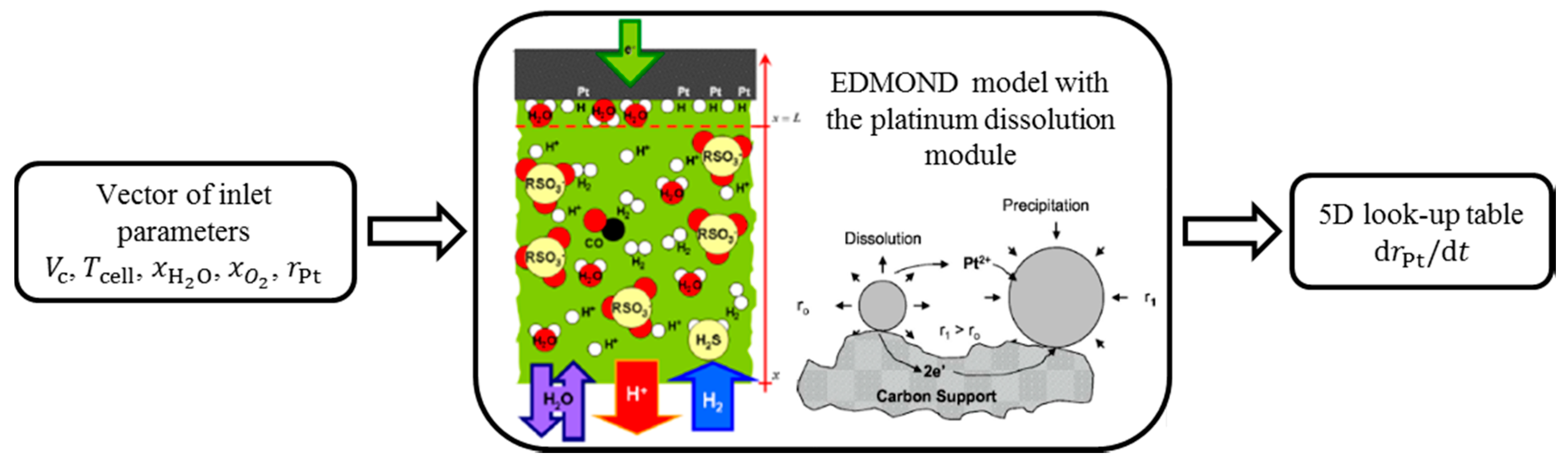
3. Pt Dissolution Model

3.1. Pt Dissolution Mechanism

The Pt dissolution model in this work is taken from Robin, Gerard et al. [26,27]. It is based on an electro-chemical dissolution reaction as:

$$\mathrm{Pt}\rightleftharpoons {\mathrm{Pt}}^{2+}+2{\mathrm{e}}^{-},$$

(3)

which consists of the following two intermediate reactions [34]:

$$\mathrm{Pt}+{\mathrm{H}}_2\mathrm{O}\rightleftharpoons \mathrm{PtO}+2{\mathrm{H}}^{+}+2{\mathrm{e}}^{-}$$

(4)

$$\mathrm{PtO}+2{\mathrm{H}}^{+}\rightleftharpoons {\mathrm{Pt}}^{2+}+{\mathrm{H}}_2\mathrm{O}.$$

(5)

The Pt dissolution is considered a three-step process [26] where firstly a Pt atom is extracted from the Pt crystal lattice and placed on the reactive site, then it undergoes an electrochemical oxidation to ${\mathrm{Pt}}^{2+}$, and finally the ${\mathrm{Pt}}^{2+}$ is desorbed from the reaction site. The total Gibbs energy of the $\mathrm{Pt}$ dissolution reaction $\Delta G=\Delta G_{\mathrm{s}}+\Delta G_{\mathrm{elec}}+\Delta G_{\mathrm{des}}$ therefore consists of three terms:

• The free energy of Pt extraction from Pt crystal lattice, $\Delta G_{\mathrm{s}}$: This free energy is calculated from density functional theory (DFT) which takes into account of the coverage of the intermediate species that depend upon the amount of hydration.
• The free energy of Pt oxidation, $\Delta G_{\mathrm{elec}}$: This is calculated from the local potential based on transition state theory (TST) as $\Delta G_{\mathrm{elec}}=-2{\alpha }_{\mathrm{Pt}}\mathrm{F}\Delta \chi$, where ${\alpha }_{\mathrm{Pt}}$ is the symmetry factor of the Pt dissolution reaction and $\Delta \chi$ is the local potential at the catalyst surface (calculated by the EDMOND model [26]).
• The free energy of ${\mathrm{Pt}}^{2+}$ desorption, $\Delta G_{\mathrm{des}}$: This is calculated as, $\Delta G_{\mathrm{des}}=-\beta E_{\mathrm{GT}}\left(r_{\mathrm{Pt}}\right)$ from $\beta$, the transfer coefficient and $E_{\mathrm{GT}}\left(r_{\mathrm{Pt}}\right),$ the Gibbs Thomson energy [35] which depends of the particle radius and is given by:

  $$E_{\mathrm{GT}}\left(r_{\mathrm{Pt}}\right)=2{\gamma }_{\mathrm{Pt}}\frac{M_{\mathrm{Pt}}}{{\rho }_{\mathrm{Pt}}{r}_{\mathrm{Pt}}},$$

  (6)

  with ${\gamma }_{\mathrm{Pt}}$ as the surface energy of Pt[111], $M_{\mathrm{Pt}}$ the molar mass of $\mathrm{Pt}$, ${\rho }_{\mathrm{Pt}}$ the mass density of $\mathrm{Pt}$, and $r_{\mathrm{Pt}}$ the $\mathrm{Pt}$ particle radius. The dependence of the $E_{\mathrm{GT}}$ on the reciprocal of platinum radius $r_{\mathrm{Pt}}$ shows that small particles are dissolved faster than the larger particles.

Table 3 contains the values of the parameters used in the $\mathrm{Pt}$ dissolution model. Overall, the kinetic rate of the Pt dissolution, $v_{\mathrm{diss}}$ is given by [26]:

$$v_{\mathrm{diss}}=k{\mathrm{e}}^{-\frac{\Delta G}{\mathrm{R}T}}=k{\mathrm{e}}^{\frac{1}{\mathrm{R}T}\left(-\Delta G_{\mathrm{s}}+2\alpha F\Delta \chi +\beta E_{\mathrm{GT}}\right)},$$

(7)

where, $k$ is a kinetic constant. $\Delta \chi$ is the local electrode potential calculated by the EDMOND model (see below) from the local cell voltage that is provided by the computational fluid dynamics (CFD) model [36]. Moreover, the other depending parameters are the temperature and the oxygen and water mole fraction as illustrated in Figure 4. Finally, the rate of change in $\mathrm{Pt}$ particle radius is calculated as:

$$\frac{\mathrm{d}{r}_{\mathrm{Pt}}}{\mathrm{d}t}=-v_{\mathrm{diss}}\frac{M_{\mathrm{Pt}}}{{\rho }_{\mathrm{Pt}}}.$$

(8)

The Pt dissolution module is implemented in the EDMOND code [26]. EDMOND is a 1D double layer model. The model calculates the $\Delta \chi$ as well as the coverage of the various reaction intermediates, based on a dynamic coupling between the local operating conditions, that is, the cathode potential $V_{\mathrm{c}}$, the local temperature $T$, the local water vapor fraction $x_{{\mathrm{H}}_2\mathrm{O}}$, the local oxygen fraction $x_{{\mathrm{O}}_2}$, the particle radius $r_{\mathrm{Pt}}$, and the kinetics of the intermediate reaction steps of Pt dissolution [37]. Both the surface potential and the coverage are involved in the mechanistic model. The Pt dissolution model used in this paper has been partially validated on 2000 h of durability tests [26]. With the help of EDMOND coupled with the Pt dissolution model, a look-up table was calculated, describing the evolution of the particle radius as a function of the local operating conditions (cf. Figure 4).

Thus our coupling of the mechanistic degradation model with the cell performance model at the macroscale relies on the use of a look-up table generated at the nanoscale as shown above. To generate the look-up table more than 2500 simulations have been computed. Several look-up tables can be used in parallel with different initial Pt particle radius, to take into account an initial size distribution.

In this catalyst degradation model, we have not considered the effect of voltage cycling on Pt degradation as observed previously [38,39,40]. Consequently, the effect of the magnitude of cathodic scans [40,41,42,43] (increasing potential or braking the vehicle), or anodic scans (decreasing potential or accelerating the vehicle) is also not considered. However, in the present driving loads, the breaking and acceleration do not contain a significant part of driving time and are very fast (equivalent to fast voltage scanning). The present degradation model also does not consider the particle growth due to redeposition (Ostwald ripening) [27,44] effect of Pt particle size distribution, and the effect of Pt loading on the cell durability. As it is known that at low ECSA the voltage loss is also influenced by transport and the structure of the CL [32,45], such an effect is not considered in this work. However, the degradation framework is presented here is flexible to include the mentioned degradation models, which will be a part of future investigations.

3.2. Integration of Pt Dissolution into Degradation Library

In this study, the reduction in the exchange current density due to the loss in ECSA is accounted by $i_0=f_{\mathrm{deg},\mathrm{C}}{i}_{0,\mathrm{init}}$, where $i_{0,\mathrm{init}}$ is the performance function that depends upon the operating conditions via $i_{\mathrm{Pt}}$ as:

$$i_{0,\mathrm{init}}=s_{\mathrm{Pt}}{w}_{\mathrm{Pt}}{u}_{\mathrm{Pt}}{i}_{\mathrm{Pt}},$$

(9)

where, $i_{\mathrm{Pt}}$ is the Pt specific current density in $\mathrm{A}/{\mathrm{cm}}^2$, $s_{\mathrm{Pt}}=1100 {\mathrm{cm}}^2/\mathrm{mg}$ is the specific area of Pt, $w_{\mathrm{Pt}}=0.15 \mathrm{mg}/{\mathrm{cm}}^2$ is the Pt loading in the catalyst layer, and $u_{\mathrm{Pt}}=0.9$ is the utilization of Pt in a Pt/C catalyst. The Pt specific current density ($i_{\mathrm{Pt}}$) represents the ORR kinetics at the Pt surface and is a function of the operating temperature and reactant concentrations given as [38]:

$$i_{\mathrm{Pt}}=i_{\mathrm{Pt},353}{\mathrm{e}}^{\frac{E_{\mathrm{act}}}{\mathrm{R}} \left(\frac{1}{T}-\frac{1}{353}\right)}{\left(\frac{p_{\mathrm{c}}{x}_{{\mathrm{O}}_2}}{\mathrm{R}T{c}_{\mathrm{ref}}}\right)}^{\left(1-{\alpha }_{\mathrm{ORR}}\right)/2}{a}_{+}^{1-2{\alpha }_{\mathrm{ORR}}},$$

(10)

where, $i_{\mathrm{Pt},353}$ is a fitting parameter, $p_{\mathrm{c}}$ is the cathode pressure, $x_{{\mathrm{O}}_2}$ is the mole fraction of oxygen, $c_{\mathrm{ref}}$ is the bulk concentration of reacting species, $\mathrm{R}$ is the universal gas constant, $T$ is the cell operating temperature, $a_{+}$ is the protonic activity, and ${\alpha }_{\mathrm{ORR}}$ is ORR symmetry factor modeled by Bao et al. [28]. The catalyst degradation factor ($f_{\mathrm{deg},\mathrm{C}}$) is defined as:

$$f_{\mathrm{deg},\mathrm{C}}=\frac{\mathrm{ECSA}}{{\mathrm{ECSA}}_{\mathrm{init}}}=\frac{s_{\mathrm{Pt}}{w}_{\mathrm{Pt}}{u}_{\mathrm{Pt}}}{s_{\mathrm{Pt},\mathrm{init}}{w}_{\mathrm{Pt},\mathrm{init}}{u}_{\mathrm{Pt},\mathrm{init}}},$$

(11)

Our present degradation mechanism does not account for transport of dissolved Pt ions within or away from the catalyst layer. Hence, the Pt loading ($w_{\mathrm{Pt}}$) of the catalyst layer is considered to be constant. Moreover, although catalyst utilization has been observed to change with changes in specific activity of Pt [46], for simplicity, we have assumed constant catalyst utilization while using the changes in $s_{Pt}$ to reflect the total changes in ECSA. Further, we have assumed spherical Pt particles represent Pt surface as a function of the radius. So, under the present set of assumptions, Equation (11) can be reduced to:

$$f_{\mathrm{deg},\mathrm{C}}=\frac{s_{\mathrm{Pt}}}{s_{\mathrm{Pt},\mathrm{init}}}=\frac{r^2}{r_{\mathrm{init}}^2}.$$

(12)

Further, we have assumed a fixed Pt radius that will help us focus on the operating condition induced Pt loss across the catalyst layer. Although, using a distribution of particle size families might be realistic, it might scale up the complexity of the study. Further, it is difficult to find reliable data on Pt particle size distribution in catalyst layer as a function of Pt loading or ECSA in the literature.

As discussed above, the Pt dissolution model provides a look-up table of the rate of change of Pt particle radius as a function of cathode potential, temperature, oxygen mole fraction, local humidity, and current Pt radius. So we can re-write the Equation (8) as a look-up table (LUT) interface with the mentioned inputs as:

$$\frac{\mathrm{d}{r}_{\mathrm{Pt}}}{\mathrm{d}t}=\mathrm{LUT}\left(V_{\mathrm{c}},T_{\mathrm{cell}},x_{{\mathrm{O}}_2},x_{{\mathrm{H}}_2\mathrm{O}},r_{\mathrm{Pt}}\right).$$

(13)

The LUT is a 5D table that gives the rate of Pt dissolution as a function of parameters with their range as, cell temperature in {343, 348, 353, 358, 363} K, cathode voltage in {0.3, 0.4, 0.5, 0.6, 0.7, 0.9} V, oxygen mole fraction in {0.1, 0.15, 0.21}, water mole fraction in {0.3, 0.5, 0.7, 0.99}, and Pt radius in {0.5, 0.75, 1.0, 1.5, 2.0, 3} nm. The intermediate values were interpolated and the values out of the range were extrapolated linearly. The Pt dissolution model uses cathode voltage, oxygen mole fraction, water mole fraction and cell temperature (constant) from the CFD model and shown in Equation (13).

The rate of change of Pt radius is integrated over the solver time-step to calculate the change in the current Pt radius. The Pt radius is then updated and used to calculate the current state of catalyst degradation factor. The new exchange current density is modified using this degradation factor as mentioned above.

3.3. Fuel Cell Durability Estimation under Pt Dissolution

Here, the time upscaling methodology mentioned above is used for estimating the ECSA loss over time through the loss is Pt radius. The upscaled loss in Pt radius at the end of ‘n’ cycles is subtracted from the Pt radius at the beginning of the cycle simulation to obtain the Pt radius at the end of ‘n’ driving cycles:

$$r_{\mathrm{Pt}}\left(t+n·t_{\mathrm{DC}}\right)=r_{\mathrm{Pt}}\left(t\right)-n·{\int }_t^{t+t_{\mathrm{DC}}}\frac{\mathrm{d}{r}_{\mathrm{Pt}}}{\mathrm{d}t}\mathrm{d}t,$$

(14)

where, $n$ is taken to be 100, which for NEDC corresponds to 33 h and for WLTC corresponds to 50 h. It is further refined to 15 towards the EOL for a better estimation of the cell behavior as it reaches the EOL. It has to be noted that the unrefined upscaling jump corresponds to the real simulation time of each driving cycle.

4. Results and Discussion

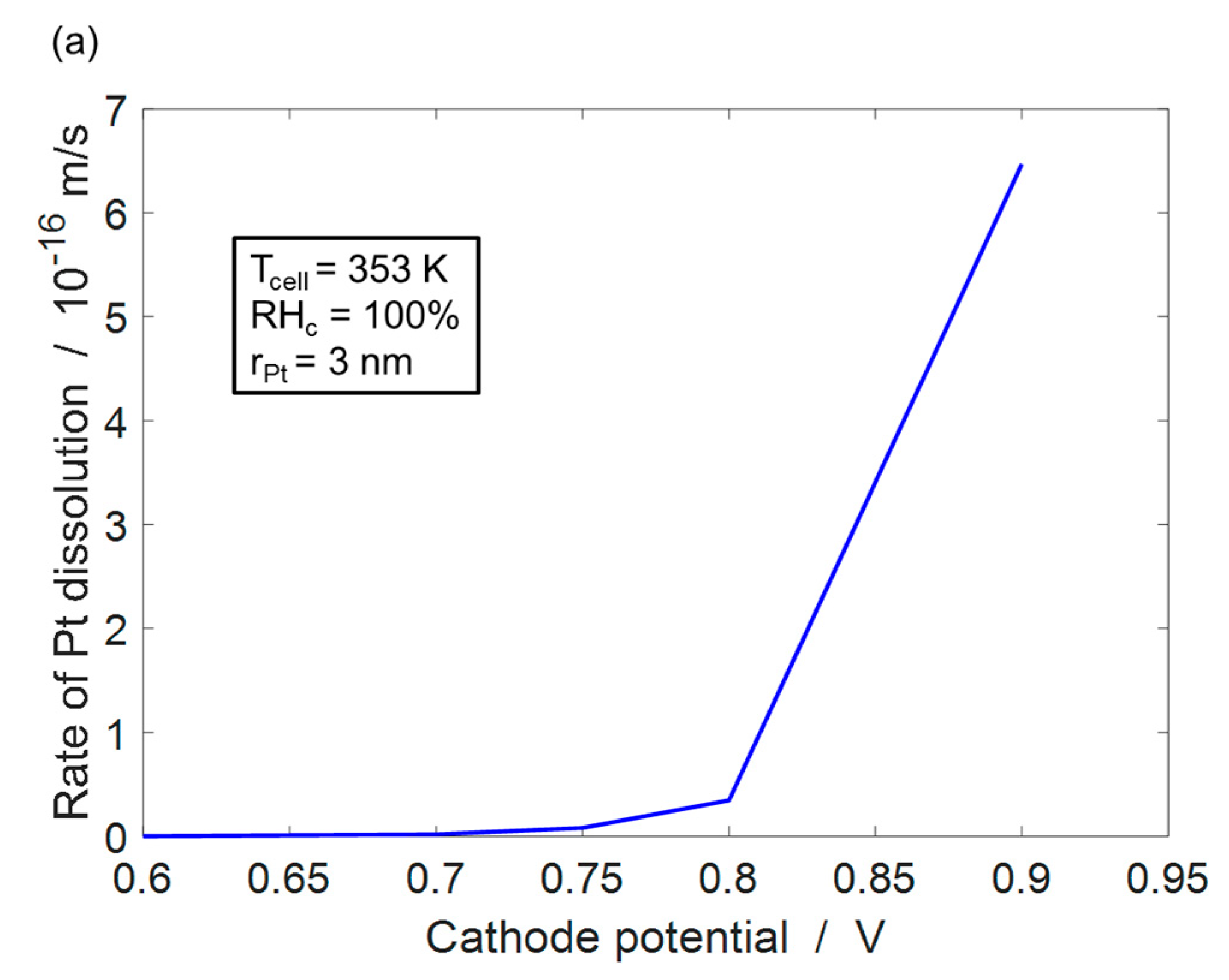
4.1. Pt Dissolution Model

The physically based Pt dissolution model has been qualitatively validated with good agreement with the Pt dissolution sensitivities on local conditions (voltage, temperature, humidity, etc.) by Robin et al. [26]. Figure 5 shows the variation of the rate of Pt dissolution with cathode potential and for a Pt particle of radius 3 nm and keeping air humidity in cathode, ${\mathrm{RH}}_{\mathrm{c}}$ at 100%. Figure 5a shows that the rate of Pt dissolution increases strongly for cathode potentials >0.8 V. This increase in the Pt dissolution rate for V_c > 0.8 V is in good agreement with experimental values presented by Ahluwalia et al. [4]. Figure 5b shows that the rate of Pt dissolution decreases with the temperature. Although, increasing the temperature enhances the reaction kinetics of Pt dissolution, but at a constant humidity it also increases the water vapor in the air. This leads to a reduction in the oxygen content in the catalyst layer. Consequently, the magnitude of equilibrium cathode voltage is reduced, which increases the overpotential, leading to a decrease in the rate of Pt degradation.

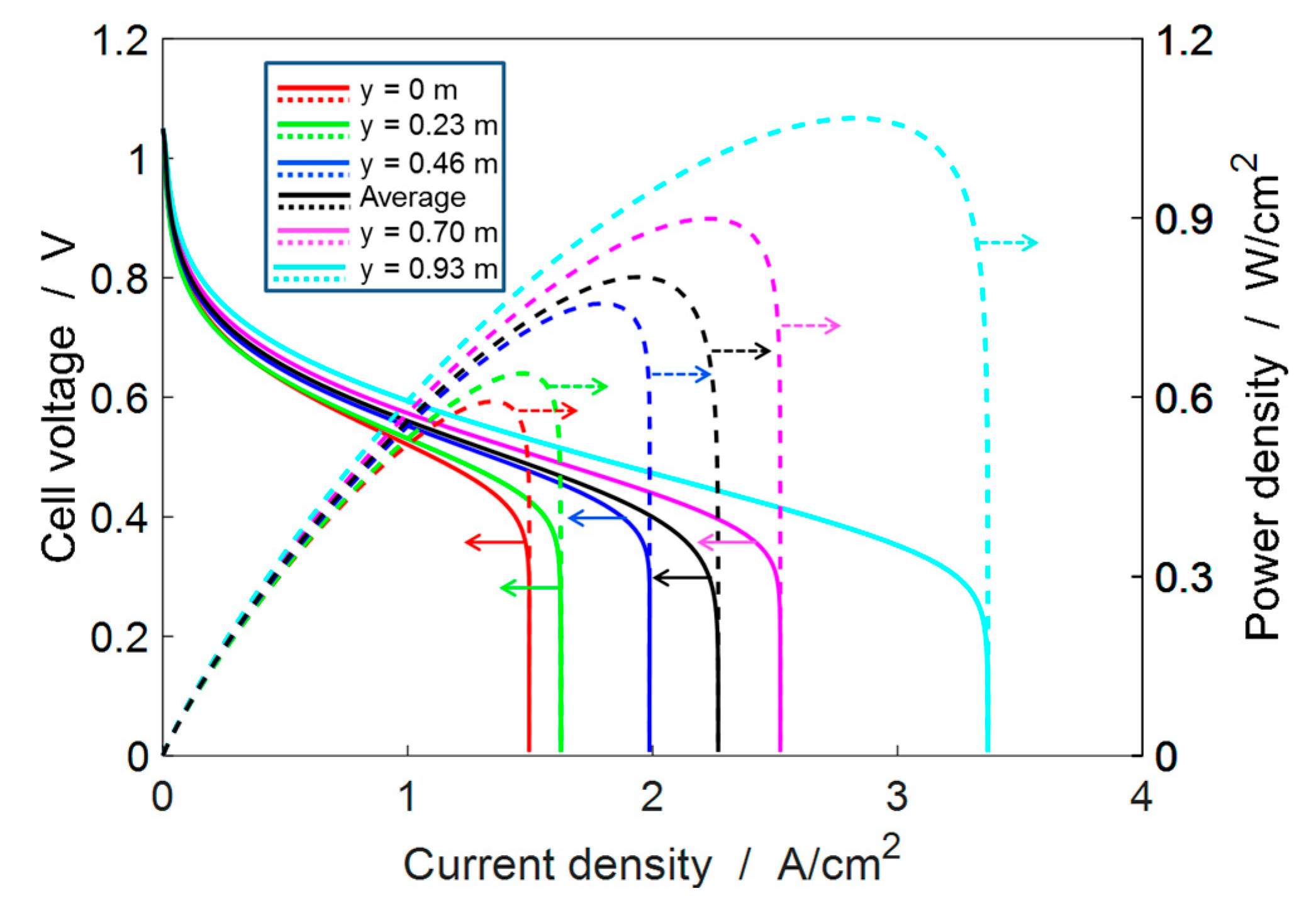
4.2. Single-Cell Performance

It is well known that single-cell performance depends strongly on the cell operating conditions. In order to do a consistent analysis of the cell performance under the two different load cycles, we have considered a standard set of operating conditions, that is, a pressure of 250 kPa, temperature of 85 °C, and 100% relative humidity. Figure 6 shows the single-cell performance under these operating conditions, where cell performance at different spatial locations along the channel is demonstrated. The cell performance shows a variable spatial dispersion, which is weaker at low current densities (<1 A/m²) and stronger at high current densities (>1 A/m²). The IV curve is obtained by polarizing the cell to the presented range of voltage and simulating the current response of the cell. Since our model is a lambda-controlled flow model, the reactant flow rate is proportional to the current demand from the cell. At high current densities, a high reactant flow rate is generated in the gas channels, causing large pressure gradients the flow direction. Hence, a spatial gradient in the reactant concentration is created, which further leads to spatially varying current density response. The maximum cell performance in the current model is observed close to the air inlet ($y=0.93 \mathrm{m}$) because it has the maximum partial pressure of oxygen. Moreover, under the given set of operating conditions, the cell can deliver a maximum average power density of 0.8 W/cm². Under the car and stack parameters considered in Table 1, the maximum single cell power density requirement by NEDC is 0.48 W/cm² and by WLTC is 0.57 W/cm². Hence, our single cell model can provide enough power for running both driving cycles.

A requirement for a fuel cell to be an efficient and robust alternative over the concurrent technologies in an automotive application is fast response to the transient power demand and high power density. To that end, we have explored the cell performance under the loading requirements of two transient automotive drive cycles. The fuel cell performance was studied under two separate driving cycles to observe the role of driver’s (controlled) behavior on the eventual durability of a fuel cell-driven car. Figure 7 shows that the transient operation of a driving cycle creates a transient power demand and consequently the fuel cell stack catering to this power demand has a transient variation in the state variables, too. If we look at the characteristics of the driving cycles (cf. Table 2), we can observe that NEDC has more idling time over the total duration (23.7%) whereas, WLTC has less of that (13.3%), so we can expect more open-circuit voltage (OCV) operations in NEDC as compared to WLTC, which suggests that a cell under WLTC load will last longer than that under NEDC cycle. One can also observe that WLTC has faster and more frequent transients leading to faster voltage cycling. The range of voltage cycling in NEDC is 1.04–0.65 V while in WLTC is 1.04–0.56 V.

Apart from cell voltage and current cycling that we can measure in situ very easily, the advantage of a 2D model is that it helps to identify the spatially resolved cell behavior under transient loadings, non-intrusively. A spatially resolved transient plot helps us to correlate the nature of changes in the cell state variable with different drive cycle conditions such as acceleration, deceleration, cruising and start/stop. Due to the presence of multiple complex interdependent physico-chemical phenomena (electrochemistry, fluid transport in open and porous media, etc.) with multiple time constants, a cell exposed to cyclic loading also undergoes cycling of other state variables such as pressure, humidity, or persistent excess or depletion of reactants, etc.

Figure 8 shows the temporal variations in mole fraction of oxygen along the cathode catalyst layer. It can be clearly observed that the time instants during the higher current densities (higher power demand) show more spatial variation in the cell state variables as compared to time instants with low current densities (low power demands). Moreover, the high mole fraction of oxygen at the air inlet ($y=0.93 \mathrm{m}$) suggests maximum current density at the location and minimum current density at the air outlet ($y=0 \mathrm{m}$). This in turn suggests that the cathodic potential (cell voltage corrected by ohmic losses, cf. the following section) is higher at the air outlet as compared to the air inlet. Further, high power demand corresponding to car acceleration leads to a sharp decline in oxygen concentration (hence, sharp change in local pressure) over a larger part of the cell. Similarly, constant cruising at a high speed leads to a longer exposure of a large part of the cell to oxygen depletion. All these phenomena can be detrimental to the performance of various components, including the Pt catalyst, which will be quantified below.

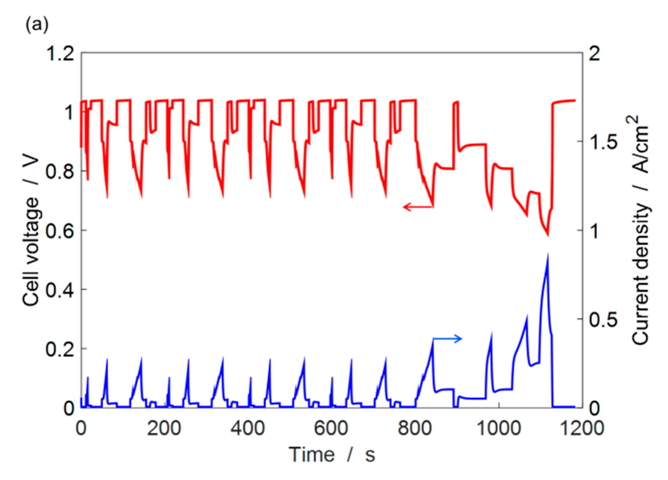
4.3. ECSA Loss under Automotive Drive Cycle

During catalyst degradation, the Pt dissolution leads to a net reduction in the ECSA in the catalyst layer. This leads to a reduction in the exchange current density and consequently increases the activation losses. Pt dissolution, hence, has an adverse effect on the performance of the fuel cell as the maximum power density provided by the cell decreases. The Pt dissolution mechanism as considered in this study has a functional dependence on the local cathode potential, temperature, humidity, and partial pressure of oxygen. Generally, the electrode consists of catalyst deposition on a carbon-based backing with a varying degree of porosity for reactant gas, so they do not contribute significantly to the ohmic losses. In our model the local cathode voltage, which is the driver for Pt dissolution, can be estimated from the cell potential by compensating it for the ohmic losses. Thus, the iR-corrected cathode potential is obtained by removing the ohmic losses from the cell voltage as:

$$V_{\mathrm{c}}=V_{\mathrm{cell}}+i_{\mathrm{cell}}{R}_{\mathrm{mem}}$$

(15)

where, $i_{\mathrm{cell}}$ is the local cell current density, and $R_{\mathrm{mem}}=\frac{l_{\mathrm{mem}}}{{\sigma }_{\mathrm{mem}}{A}_{\mathrm{cell}}}$ is the membrane resistance calculated from membrane thickness ($l_{\mathrm{mem}}$), conductivity (${\sigma }_{\mathrm{mem}}$), and surface area ($A_{\mathrm{cell}}$). Due to local variations in the cell current density and membrane conductivity, the iR-corrected cathode potential has a spatial variation. This consequently leads to a spatially varying Pt dissolution rate.

Figure 9 shows the iR-corrected cathode potential variation and the rate of Pt radius loss during the two driving cycles. The Pt dissolution rate is observed to be highest for near OCV operations. Further, in order to demonstrate the effect of spatial variation in the cell state variables on the rate of Pt radius loss, we show them at the two extremities in our cell geometry, namely, near the air outlet ($y=0 \mathrm{m}$) and near the air inlet ($y=0.93 \mathrm{m}$). For persistent low cell voltages (high speed cruising), some difference in rate of Pt radius loss is observed at the air inlet and outlet. For the rest of the situations such as low speed cruising, acceleration and deceleration, we do not observe any noticeable spatial variation in the rate of Pt radius loss.

Figure 10 shows that the time-averaged (over one driving cycle) spatial distributions of iR-corrected cathode potential and rate of Pt dissolution for both driving cycles. One can observe small potential gradients near the air outlet over the duration of a driving cycle. This is due to significant changes in reactant concentration near the outlet over the highly fluctuating current demand during the driving cycle. Consequently, the rate of Pt dissolution also shows spatial gradients near the outlet. Further, one can also observe that the two driving cycles have different effects on the mean degradation rate at a given location. The NEDC with higher idling time leads to more near OCV operations as compared to the WLTC, and hence has a higher mean voltage and consequently, higher rate of Pt dissolution.

4.4. Durability Estimation

It is known that the cell output power density diminishes under degradation. Figure 11 shows the maximum power density that can be generated by the single cell modeled in this work, which is the maximum of the P/i curve, at different amounts of ECSA loss (defined by the catalyst degradation factor). It can be seen that there is a drastic non-linear reduction in the cell performance after the cell loses approx. 30% of its ECSA. Since, the objective of our cell is to provide the power demanded by a driving cycle, in order to completely execute a driving cycle test it must be able to provide the maximum power required by the cycle. If the cell under increasing degradation is not able to provide the power required, we can say that the cell has achieved its end-of-life. As discussed previously, the maximum power demand by WLTC is 0.57 W/cm² and NEDC is 0.48 W/cm². It is observed from the figure that the cell power density output fails to match the maximum power demands for WLTC and NEDC below catalyst degradation factors of 0.24 and 0.13, respectively. In other words, with the help of the figure, we can estimate that under the same set of operating conditions, a cell working under WLTC will fail earlier than a cell working under NEDC.

One of the easily measurable indicators of cell health is cell voltage. Figure 12 shows the change in (a) cell voltage corresponding to the maximum power density demanded by the driving cycle (NEDC: 1116 s, WLTC: 1569 s) and (b) catalyst degradation factor with time under NEDC and WLTC. It can be seen that the cell voltage decreases non-linearly and drops suddenly towards the end of life. This demonstrates that our current approach of piece-wise linear upscaling of the catalyst degradation factor allows to capture the nonlinearity of the cell degradation. Further, towards the end of life of the cell, the number of interpolating driving cycles was refined from 100 to 15, to closely approach the cell failure limit for both the driving cycles. In the simulation time scale, this corresponds to a reduction of drive cycle interpolation time from 33 h to 5 h for NEDC and from 50 h to 7.5 h for WLTC. For the NEDC, the predicted end of life is ca. 436–441 h and for WLTC, it is ca. 508–515 h. The end of life is proposed as a range, where the minimum value of the range corresponds to the time taken for the last successfully completed driving cycle, and the maximum value of the time-range corresponds to the linearly upscaled time through which the degradation factor fell below the minimum physical value required for the numerical convergence of the model.

Figure 13 shows the distribution of Pt radius towards the end of life of the fuel cell. For the NEDC, the Pt radius at 436 h is 1.09 nm, which means that there is ~87% loss in Pt surface area after 872 NEDC loads (one NEDC is 1180 s). For WTLC, the Pt radius at 500 h is 1.63 nm, which means that there is ~70% loss in Pt surface area after 1000 WLTC loads (one WLTC is 1800 s). Figure 9a shows that during one NEDC, 19 cell voltage plateaus are occurring corresponding to a cell voltage of 1.04 V. We can compare these results to experimental data by Yang et al. [47], who use a square wave voltage profile between 0.4–1.05 V and observed an ECSA loss of ca. 60% during 10,000 cycles. The NEDC studied here could be, in a first-order abstraction, seen as a square wave voltage cycle behavior, where 19 square wave cycle equivalents between 0.62–1.04V are occurring during a single driving cycle. Hence, over 872 NEDCs, we can observe 16,568 square wave equivalent cell voltage cycles, which is in the same order of magnitude as the experiments by Yang et al. [47]. Considering the observation that smaller Pt particles dissolve faster, one could estimate greater degradation of Pt upon increasing the number of voltage cycles to 16,568 in the work by Yang. This demonstrates that the presented framework provides a comparable first-order estimate of cell durability under driving cycle loads.

Further, we find that the predicted PEMFC durability is much less than that of the standard requirement of 5000 h under an automotive dynamic load (including start and stop conditions). Both standard driving cycles (NEDC and WLTC) that were used to generate the dynamic load for the PEMFC model have a significant idling time, NEDC ~24% and WLTC ~14% (cf. Table 2). Since, our Pt dissolution model has maximum Pt dissolution rate at near OCV operations (or zero current/vehicle idling), these driving cycles induce “worst-case” environments for the CL. Note further that the degradation mechanism was parameterized against experimental data [26], so that the simulated ageing behavior represents that particular experiment. Given this, the study does provide an interesting insight in the influence of operating parameters on the PEMFC durability. This can help to identify appropriate mitigation strategies, such as, increasing the Pt loading, reducing the vehicle idling time (near OCV operation) or increasing auxiliary power demand (lights, heating, air conditioning) from the PEMFC so that near-OCV operating is avoided.

The results of Figure 13 show no significant spatial variation in the Pt radius even at the end of life of the fuel cell. This can be attributed to the observation that inhomogeneous ageing conditions are significant mainly at high current demand (cf. Figure 9), which however in turn shows low absolute degradation during the driving cycle. Further, even though some spatial gradient is observed for the rate of Pt dissolution through the channel length (cf. Figure 10), due to its small order of magnitude, no significant variation in Pt radius distribution is observed.

It has been observed in the literature that different amounts of Pt dissolution at inlet and outlet and different distributions of Pt causes significant spatially-varying ECSA loss [33,47]. This indicates that, in order to reliably model the spatially resolved cell degradation, other local degradation mechanisms must be considered. Indeed, it is known that there are many other degradation mechanisms such as loss of membrane conductivity [48,49,50], gas cross-over [51], loss of carbon in CL and GDL [52], modification of micro-porous layer (MPL) properties [53], increase in contact resistance [54], etc., which might occur either in parallel or dominate at certain times during a driving cycle. Considering such mechanisms might improve the durability prediction of this model. Although, it is very difficult to isolate the effect of individual degradation mechanism on the overall durability of the PEMFC, our study proposes a framework that can be used to combine different physically based degradation mechanisms of individual processes to improve the PEMFC durability prediction.

The present model does not spatially resolve the thickness of the CL, so an influence of local (on the CL thickness scale) degradation cannot be studied. However, the model could be extended using published approaches for microstructure and transport [55] which could be coupled with the present degradation model. The addition of a model for particle size distribution and platinum redistribution [35] would further enhance the model accuracy.

5. Conclusions

With the help of a multiscale coupling between a fuel cell car model and cell level catalyst degradation model, we were able to estimate cell durability and provide insights into spatially resolved cell performance. By analyzing the cell performance and degradation under two different kinds of drive cycles, we presented a comparative overview of different driving characteristics (accelerating, decelerating, cruising, and idling) on the behavior of local cell state variables. The role of transient loading on the spatial variations in the cell state variables, especially, iR-corrected cathode potential, the concentration of water and oxygen, and the spatial variations in the rate of Pt dissolution in the cathode catalyst layer was discussed. We found that the rate of Pt dissolution is highest for low power demand (vehicle idling) but the spatial dispersion in the rate of Pt dissolution is highest for high power demand (acceleration and high speed cruising). Comparing between two well-known drive cycles NEDC and WLTC, we observed that NEDC with longer near-OCV operation had earlier EOL than WLTC. Moreover, under the considered operating conditions, the rate of Pt dissolution shows a highly transient behavior during a driving cycle, but its spatial variation along the CCL was not so significant to result in a localized ECSA loss.

The study uses a computational time-upscaling methodology that allows for long-term (hundreds to thousands of simulation time) prediction of the PEMFC behavior based on computationally expensive multiphysics models. Overall, this study presents a flexible multiscale platform that enables to estimate EOL for a fuel cell under a driving cycle load, and propose potential design strategies and degradation mitigation techniques. Consequently, with the help of additional component degradation models, this study can be extended for a better estimation of cell durability and localized degradation under realistic loads such as in an automotive application.

References

1. Yu, X.; Ye, S. Recent advances in activity and durability enhancement of Pt/C catalytic cathode in PEMFC. J. Power Sources 2007, 172, 145–154. [Google Scholar] [CrossRef]
2. Gasteiger, H.A.; Kocha, S.S.; Sompalli, B.; Wagner, F.T. Activity benchmarks and requirements for Pt, Pt-alloy, and non-Pt oxygen reduction catalysts for PEMFCs. Appl. Catal. B Environ. 2005, 56, 9–35. [Google Scholar] [CrossRef]
3. Shao-Horn, Y.; Sheng, W.C.; Chen, S.; Ferreira, P.J.; Holby, E.F.; Morgan, D. Instability of Supported Platinum Nanoparticles in Low-Temperature Fuel Cells. Top. Catal. 2007, 46, 285–305. [Google Scholar] [CrossRef]
4. Ahluwalia, R.K.; Arisetty, S.; Wang, X.; Subbaraman, R.; Ball, S.C.; DeCrane, S.; Myers, D.J. Thermodynamics and Kinetics of Platinum Dissolution from Carbon-Supported Electrocatalysts in Aqueous Media under Potentiostatic and Potentiodynamic Conditions. J. Electrochem. Soc. 2013, 160, F447–F455. [Google Scholar] [CrossRef]
5. Virkar, A.V.; Zhou, Y. Mechanism of Catalyst Degradation in Proton Exchange Membrane Fuel Cells. J. Electrochem. Soc. 2007, 154, B540. [Google Scholar] [CrossRef]
6. Shao, Y.; Kou, R.; Wang, J.; Viswanathan, V.V.; Kwak, J.H.; Liu, J.; Wang, Y.; Lin, Y. The influence of the electrochemical stressing (potential step and potential-static holding) on the degradation of polymer electrolyte membrane fuel cell electrocatalysts. J. Power Sources 2008, 185, 280–286. [Google Scholar] [CrossRef]
7. Luo, Z.; Li, D.X.; Tang, H.; Pan, M.; Ruan, R. Degradation behavior of membrane-electrode-assembly materials in 10-cell PEMFC stack. Int. J. Hydrog. Energy 2006, 31, 1831–1837. [Google Scholar] [CrossRef]
8. Zhang, S.; Yuan, X.Z.; Hin, J.N.; Wang, H.; Friedrich, K.A.; Schulze, M. A review of platinum-based catalyst layer degradation in proton exchange membrane fuel cells. J. Power Sources 2009, 194, 588–600. [Google Scholar] [CrossRef]
9. Bi, W.; Sun, Q.; Deng, Y.; Fuller, T.F. The effect of humidity and oxygen partial pressure on degradation of Pt/C catalyst in PEM fuel cell. Electrochim. Acta 2009, 54, 1826–1833. [Google Scholar] [CrossRef]
10. Bussian, D.A.; O’Dea, J.R.; Metiu, H.; Buratto, S.K. Nanoscale current imaging of the conducting channels in proton exchange membrane fuel cells. Nano Lett. 2007, 7, 227–232. [Google Scholar] [CrossRef] [PubMed]
11. Cleghorn, S.J.C.; Derouin, C.R.; Wilson, M.S.; Gottesfeld, S. A printed circuit board approach to measuring current distribution in a fuel cell. J. Appl. Electrochem. 1998, 28, 663–672. [Google Scholar] [CrossRef]
12. Lilavivat, V.; Shimpalee, S.; van Zee, J.W.; Xu, H.; Mittelsteadt, C.K. Current Distribution Mapping for PEMFCs. Electrochim. Acta 2015, 174, 1253–1260. [Google Scholar] [CrossRef] [Green Version]
13. Durst, J.; Lamibrac, A.; Charlot, F.; Dillet, J.; Castanheira, L.F.; Maranzana, G.; Dubau, L.; Maillard, F.; Chatenet, M.; Lottin, O. Degradation heterogeneities induced by repetitive start/stop events in proton exchange membrane fuel cell: Inlet vs. outlet and channel vs. land. Appl. Catal. B Environ. 2013, 138–139, 416–426. [Google Scholar] [CrossRef]
14. Rajalakshmi, N.; Raja, M.; Dhathathreyan, K.S. Evaluation of current distribution in a proton exchange membrane fuel cell by segmented cell approach. J. Power Sources 2002, 112, 331–336. [Google Scholar] [CrossRef]
15. Schulze, M.; Gülzow, E.; Schönbauer, S.; Knöri, T.; Reissner, R. Segmented Cells as Tool for Development of Fuel Cells and Error Prevention/Prediagnostic in Fuel Cell Stacks. J. Power Sources 2007, 173, 19–27. [Google Scholar] [CrossRef]
16. Pérez, L.C.; Brandão, L.; Sousa, J.M.; Mendes, A. Segmented polymer electrolyte membrane fuel cells—A review. Renew. Sustain. Energy Rev. 2011, 15, 169–185. [Google Scholar] [CrossRef]
17. Zhang, J.; Zhang, H.; Wu, J.; Zhang, J. PEM Fuel Cell Testing and Diagnosis; Elsevier Science: Oxford, UK, 2013. [Google Scholar]
18. Wang, H.H.; Yuan, X.-Z.; Li, H. PEM Fuel Cell Diagnostic Tools; CRC Press/Taylor & Francis: Boca Raton, FL, USA, 2011. [Google Scholar]
19. Uchimura, M.; Kocha, S.S. The Impact of Cycle Profile on PEMFC Durability. ECS Trans. 2007, 11, 1215–1226. [Google Scholar]
20. Borup, R.; Davey, J.; Garzon, F.; Wood, D.; Welch, P.; More, K. PEM Fuel Cell Durability with Transportation Transient Operation. ECS Trans. 2006, 3, 879–886. [Google Scholar]
21. Schmittinger, W.; Vahidi, A. A review of the main parameters influencing long-term performance and durability of PEM fuel cells. J. Power Sources 2008, 180, 1–14. [Google Scholar] [CrossRef]
22. Borup, R.; Meyers, J.; Pivovar, B.; Kim, Y.S.; Mukundan, R.; Garland, N.; Myers, D.; Wilson, M.; Garzon, F.; Wood, D.; et al. Scientific aspects of polymer electrolyte fuel cell durability and degradation. Chem. Rev. 2007, 107, 3904–3951. [Google Scholar] [CrossRef] [PubMed]
23. Cheng, X.; Shi, Z.; Glass, N.; Zhang, L.; Zhang, J.; Song, D.; Liu, Z.-S.; Wang, H.; Shen, J. A review of PEM hydrogen fuel cell contamination: Impacts, mechanisms, and mitigation. J. Power Sources 2007, 165, 739–756. [Google Scholar] [CrossRef]
24. Jahnke, T.; Futter, G.; Latz, A.; Malkow, T.; Papakonstantinou, G.; Tsotridis, G.; Schott, P.; Gérard, M.; Quinaud, M.; Quiroga, M.; et al. Performance and degradation of Proton Exchange Membrane Fuel Cells: State of the art in modeling from atomistic to system scale. J. Power Sources 2016, 304, 207–233. [Google Scholar] [CrossRef] [Green Version]
25. Mayur, M.; Strahl, S.; Husar, A.; Bessler, W.G. A Multi-Timescale Modeling Methodology for PEMFC Performance and Durability in a Virtual Fuel Cell Car. Int. J. Hydrog. Energy 2015, 40, 16466–16476. [Google Scholar] [CrossRef] [Green Version]
26. Robin, C.; Gérard, M.; Quinaud, M.; d’Arbigny, J.; Bultel, Y. Proton exchange membrane fuel cell model for aging predictions. Simulated equivalent active surface area loss and comparisons with durability tests. J. Power Sources 2016, 326, 417–427. [Google Scholar] [CrossRef]
27. Gerard, M.; Robin, C.; Chandesris, M.; Schott, P. (Invited) Polymer Electrolyte Fuel Cells Lifetime Prediction by a Full Multi-Scale Modeling Approach. ECS Trans. 2016, 75, 35–43. [Google Scholar] [CrossRef]
28. Bao, C.; Bessler, W.G. Two-Dimensional Modeling of a Polymer Electrolyte Membrane Fuel Cell with Long Flow Channel. Part I. Model development. J. Power Sources 2015, 275, 922–934. [Google Scholar] [CrossRef]
29. United Nations UNECE. Agreement Concerning the Adoption of Uniform Technical Prescriptions for Wheeled Vehicles, Equipment and Parts Which Can Be Fitted and/or Be Used on Wheeled Vehicles and the Conditions for Reciprocal Recognition of Approvals Granted on the Basis of These Prescriptions. Available online: http://digitallibrary.un.org/record/492895 (accessed on 17 September 2015).
30. Tutuianu, M.; Marotta, A.; Steven, H.; Ericsson, E.; Haniu, T.; Ichikawa, N.; Ishii, H. Development of a World-Wide Worldwide Harmonized Light Duty Driving Test Cycle (WLTC). Available online: https://www.unece.org/fileadmin/DAM/trans/doc/2014/wp29grpe/GRPE-68-03e.pdf (accessed on 17 September 2015).
31. Martin, A.; Joerissen, L. Auto-Stack—Implementing a European Automotive Fuel Cell Stack Cluster. ECS Trans. 2012, 42, 31–38. [Google Scholar]
32. Owejan, J.P.; Owejan, J.E.; Gu, W. Impact of Platinum Loading and Catalyst Layer Structure on PEMFC Performance. J. Electrochem. Soc. 2013, 160, F824–F833. [Google Scholar] [CrossRef]
33. Li, Y.; Moriyama, K.; Gu, W.; Arisetty, S.; Wang, C.Y. A One-Dimensional Pt Degradation Model for Polymer Electrolyte Fuel Cells. J. Electrochem. Soc. 2015, 162, F834–F842. [Google Scholar] [CrossRef]
34. Robin, C.; Gerard, M.; Franco, A.A.; Schott, P. Multi-scale coupling between two dynamical models for PEMFC aging prediction. Int. J. Hydrog. Energy 2013, 38, 4675–4688. [Google Scholar] [CrossRef]
35. Holby, E.F.; Sheng, W.; Shao-Horn, Y.; Morgan, D. Pt nanoparticle stability in PEM fuel cells. Influence of particle size distribution and crossover hydrogen. Energy Environ. Sci. 2009, 2, 865. [Google Scholar] [CrossRef]
36. Franco, A.A.; Schott, P.; Jallut, C.; Maschke, B. A Multi-Scale Dynamic Mechanistic Model for the Transient Analysis of PEFCs. Fuel Cells 2007, 7, 99–117. [Google Scholar] [CrossRef] [Green Version]
37. Franco, A.A.; Passot, S.; Fugier, P.; Anglade, C.; Billy, E.; Guétaz, L.; Guillet, N.; de Vito, E.; Mailley, S. PtxCoy Catalysts Degradation in PEFC Environments: Mechanistic Insights. J. Electrochem. Soc. 2009, 156, B410. [Google Scholar] [CrossRef]
38. Ferreira, P.J.; Shao-Horn, Y.; Morgan, D.; Makharia, R.; Kocha, S.; Gasteiger, H.A. Instability of Pt/C electrocatalysts in proton exchange membrane fuel cells—A mechanistic investigation. J. Electrochem. Soc. 2005, 152, A2256–A2271. [Google Scholar] [CrossRef]
39. Redmond, E.L.; Setzler, B.P.; Juhas, P.; Billinge, S.J.L.; Fuller, T.F. In-Situ Monitoring of Particle Growth at PEMFC Cathode under Accelerated Cycling Conditions. Electrochem. Solid-State Lett. 2012, 15, B72. [Google Scholar] [CrossRef]
40. Mitsushima, S.; Kawahara, S.; Ota, K.-I.; Kamiya, N. Consumption Rate of Pt under Potential Cycling. J. Electrochem. Soc. 2007, 154, B153. [Google Scholar] [CrossRef]
41. Cherevko, S.; Zeradjanin, A.R.; Keeley, G.P.; Mayrhofer, K.J.J. A Comparative Study on Gold and Platinum Dissolution in Acidic and Alkaline Media. J. Electrochem. Soc. 2014, 161, H822–H830. [Google Scholar] [CrossRef] [Green Version]
42. Jovanovič, P.; Pavlišič, A.; Šelih, V.S.; Šala, M.; Hodnik, N.; Bele, M.; Hočevar, S.; Gaberšček, M. New Insight into Platinum Dissolution from Nanoparticulate Platinum-Based Electrocatalysts Using Highly Sensitive In Situ Concentration Measurements. ChemCatChem 2014, 6, 449–453. [Google Scholar] [CrossRef]
43. Lopes, J.A.P.; Moreira, C.L.; Madureira, A.G. Defining Control Strategies for MicroGrids Islanded Operation. IEEE Trans. Power Syst. 2006, 21, 916–924. [Google Scholar] [CrossRef] [Green Version]
44. Parthasarathy, P.; Virkar, A.V. Electrochemical Ostwald ripening of Pt and Ag catalysts supported on carbon. J. Power Sources 2013, 234, 82–90. [Google Scholar] [CrossRef]
45. Weber, A.Z.; Kusoglu, A. Unexplained transport resistances for low-loaded fuel-cell catalyst layers. J. Mater. Chem. A 2014, 2, 17207–17211. [Google Scholar] [CrossRef]
46. Bose, A.; Babburi, P.; Kumar, R.; Myers, D.; Mawdsley, J.; Milhuff, J. Performance of individual cells in polymer electrolyte membrane fuel cell stack under-load cycling conditions. J. Power Sources 2013, 243, 964–972. [Google Scholar] [CrossRef]
47. Yang, Z.; Ball, S.; Condit, D.; Gummalla, M. Systematic Study on the Impact of Pt Particle Size and Operating Conditions on PEMFC Cathode Catalyst Durability. J. Electrochem. Soc. 2011, 158, B1439. [Google Scholar] [CrossRef]
48. Coms, F.D. The Chemistry of Fuel Cell Membrane Chemical Degradation. ECS Trans. 2008, 16, 235–255. [Google Scholar] [Green Version]
49. Coulon, R.; Bessler, W.; Franco, A.A. Modeling Chemical Degradation of a Polymer Electrolyte Membrane and its Impact on Fuel Cell Performance. ECS Trans. 2010, 25, 259–273. [Google Scholar]
50. Ghelichi, M.; Melchy, P.-É.A.; Eikerling, M.H. Radically coarse-grained approach to the modeling of chemical degradation in fuel cell ionomers. J. Phys. Chem. B 2014, 118, 11375–11386. [Google Scholar] [CrossRef] [PubMed]
51. Cheng, X.; Zhang, J.; Tang, Y.; Song, C.; Shen, J.; Song, D.; Zhang, J. Hydrogen crossover in high-temperature PEM fuel cells. J. Power Sources 2007, 167, 25–31. [Google Scholar] [CrossRef]
52. Park, J.; Oh, H.; Ha, T.; Lee, Y.I.; Min, K. A review of the gas diffusion layer in proton exchange membrane fuel cells: Durability and degradation. Appl. Energy 2015, 155, 866–880. [Google Scholar] [CrossRef]
53. Lapicque, F.; Belhadj, M.; Bonnet, C.; Pauchet, J.; Thomas, Y. A critical review on gas diffusion micro and macroporous layers degradations for improved membrane fuel cell durability. J. Power Sources 2016, 336, 40–53. [Google Scholar] [CrossRef]
54. Papadias, D.D.; Ahluwalia, R.K.; Thomson, J.K.; Meyer, H.M.; Brady, M.P.; Wang, H.; Turner, J.A.; Mukundan, R.; Borup, R. Degradation of SS316L bipolar plates in simulated fuel cell environment: Corrosion rate, barrier film formation kinetics and contact resistance. J. Power Sources 2015, 273, 1237–1249. [Google Scholar] [CrossRef] [Green Version]
55. Eikerling, M. Water management in cathode catalyst layers of PEM fuel cells. J. Electrochem. Soc. 2006, 153, E58–E70. [Google Scholar] [CrossRef]
Figure 1. Schematics of the simulation framework with various interacting sub-components and their interfacing parameters.
Energies 11 02054 g001
Figure 2. Velocity and power cycling during different driving cycles used in the current work, (a) NEDC; and (b) WLTC.
Energies 11 02054 g002
Figure 3. Two-dimensional computational domain of the single-cell model. Solid boundaries are no-flux boundaries. The beginning ( y = 0   m ) and the end ( y = 0.93   m ) of representative section boundaries are shown with dashed blue lines. Not to scale.
Energies 11 02054 g003
Figure 4. Schematic illustration of the calculation of degradation look-up table.
Energies 11 02054 g004
Figure 5. Variation of the rate of Pt loss with respect to the input parameters (a) cathode voltage; and (b) cell temperature.
Energies 11 02054 g005aEnergies 11 02054 g005b
Figure 6. Single-cell performance at a pressure of 250 kPa, temperature of 85 °C, and 100% relative humidity. The IV curve is obtained by polarizing the cell to a monotonically decreasing voltage and obtaining the current and power densities at different spatial locations along the y-axis (cf. Figure 3). The average cell performance is shown by the black line.
Energies 11 02054 g006
Figure 7. Cell voltage and current density during different driving cycles, (a) NEDC; and (b) WLTC.
Energies 11 02054 g007aEnergies 11 02054 g007b
Figure 8. Spatial variation in mole fraction of oxygen along the CCL (y-axis in Figure 3) during (a) NEDC; and (b) WLTC.
Energies 11 02054 g008
Figure 9. Voltage cycling and rate of Pt dissolution observed under different driving cycles (a) NEDC; and (b) WLTC, at air outlet ( y = 0   m ) and air inlet ( y = 0.93   m ).
Energies 11 02054 g009
Figure 10. Spatial variation in the iR-corrected cathode potential and the rate of Pt dissolution averaged over the duration of one driving cycle.
Energies 11 02054 g010
Figure 11. Maximum single cell power density at different values of catalyst degradation factor. The maximum single cell power density demand by WLTC and NEDC and corresponding minimum degradation factor is marked.
Energies 11 02054 g011
Figure 12. Decrease in (a) cell voltage corresponding to the maximum power and (b) catalyst degradation factor over time under various driving cycles.
Energies 11 02054 g012
Figure 13. Pt radius distribution in the cathode catalyst layer at different times for (a) NEDC; and (b) WLTC.
Energies 11 02054 g013