Energy Retrofitting Strategies and Economic Assessments: The Case Study of a Residential Complex Using Utility Bills

Abstract

Promotion of retrofit actions on existing buildings is a goal in Italy, since most of them were built before the 80′s when little attention was paid to energy saving. This paper presents an integrated passive design approach to reduce the heating demand and limit the costs of a representative existing residential complex located in Bologna, in the northern part of Italy. To this purpose, we explored different scenarios upon actions taken on the building structure: (1) High efficiency windows; (2) additional insulation on the external walls; or (3) the simultaneous application of high efficiency windows and improved thermal envelope, on both external walls and roofing. The numerical optimization has been performed dynamically using TRNSYS simulation tool, to evaluate energy consumptions in different structural conditions. Then, the developed model has been calibrated by the real consumption data deduced from energy bills (years 2009–2015). Finally, the energy results obtained in the above mentioned different scenarios have been evaluated under an economic assessment of cost investment: It has been highlighted that the payback time (PBT) results to be strongly influenced by the national policies of fiscal incentives. According to the present model, the most profitable condition is obtained when additional insulation on the external walls is applied: The total amount of energy saving resulted to be equal to 930.4 MWh, with an optimal PBT of roughly six years, when tax refund was contemplated.

1. Introduction

European countries agreed on a new level target of 30% for improving energy efficiency by 2030 [1]. A series of accompanying initiatives on energy efficiency will ensure that the target can be delivered cost-efficiently, by adapting the relevant legislation to a 2030 context and tackling the multiple barriers holding back investments in energy efficiency and, in particular, in the renovation of buildings [2]. In the European Union (EU), the building sector covers 40% of the total energy consumption, resulting in 36% of CO₂ gas emissions [3]. In future projection, it is expected that residential buildings account for 25% of the final energy consumption in the EU [3]. Consequently, an urgent require to apply sustainability concepts to the design and construction of buildings has emerged. Although future buildings can be designed to decrease their energy consumption, existing buildings still make up the largest portion of buildings in service [4,5]. Building energy system is analyzed in literature through several approaches. A multi-objective of building energy system with retrofitting is applied for a case study [6] of typical residential buildings in the Swiss village of Zernez. Although common solutions in energy systems and retrofit option have been outlined, the results have indicated different optimization strategies for retrofitting depending on building category (age, size etc.). Delmastro et al. [7] studied cost optimal energy retrofit policies for residential buildings at urban scale, considering also the implication of socio-economic aspects on policies implementation. In Europe, a substantial share of the building stock is older than 50 years: More than 40% of our residential buildings have been constructed before the Sixties when the energy regulations were very limited or even absent [8,9]. Therefore, the promotion of proper retrofit actions on existing buildings has focused the interest of large part of the scientific community. The design of a building energy retrofit is a challenging assignment that requires an integrated team approach because conflicting objectives generally persist [10], i.e., the minimization of energy consumption and the maximization of economic benefits. This is the reason why a multi-objective optimization approach is commonly recommended in literature [11,12,13]. Marrone et al. investigated [14] proper cost-effective strategies applied to educational buildings for retrofitting. A sample composed of 80 school buildings characterized by different features (construction age, technologies) was investigated, taking into account the following interventions: (i) Envelope insulations, (ii) energy service upgrades, and (iii) renewable energy sources implementation. The proposed approach proved to be useful also to define reference buildings used as a model for evaluating the persistence over time of further margins for energy savings. The studies reported in Refs. [15,16,17] are based on economic assessments. In particular, Cucchiella et al. [17] recounted a sensitivity analysis (to check the assumptions of a set of input variables) that will be taken as a model for the treatment in the next part of this paper. The present paper deals with an integrated passive design approach to reduce the heating demand for an existing residential complex located in Bologna (Figure 1), in the northern part of Italy, and constructed in 1972. The numerical procedure has been performed dynamically by means of TRNSYS simulation tool [18]. The retrofitting actions here investigated are windows replacement, external walls additional insulation, and simultaneously all the retrofit solutions of high efficiency windows and improved thermal envelope (external walls and roofing). The above-mentioned measure of improved thermal envelope is motivated by the statement that 50% of a building’s total energy consumption is dissipated through its walls and roofs [19]. Referring to a low energy building (LEB), high insulation level also increases the weight of heat gains from lighting and solar radiation. Due to lower U-value materials in LEBs, it reduces the indoor temperature fluctuations throughout the day resulting in a sort of equilibrium indoor climate. In addition to this, the lower U-value augments the thermal resistance of the building by resulting in a slower heat transfer between the walls and indoor and introduces a large time constant. The retrofit action based on high efficiency windows that has been initially developed here was considered because a number of studies [20,21,22] have indicated that the effect of windows on energy consumption may change drastically with improved insulation levels, especially in residential buildings.

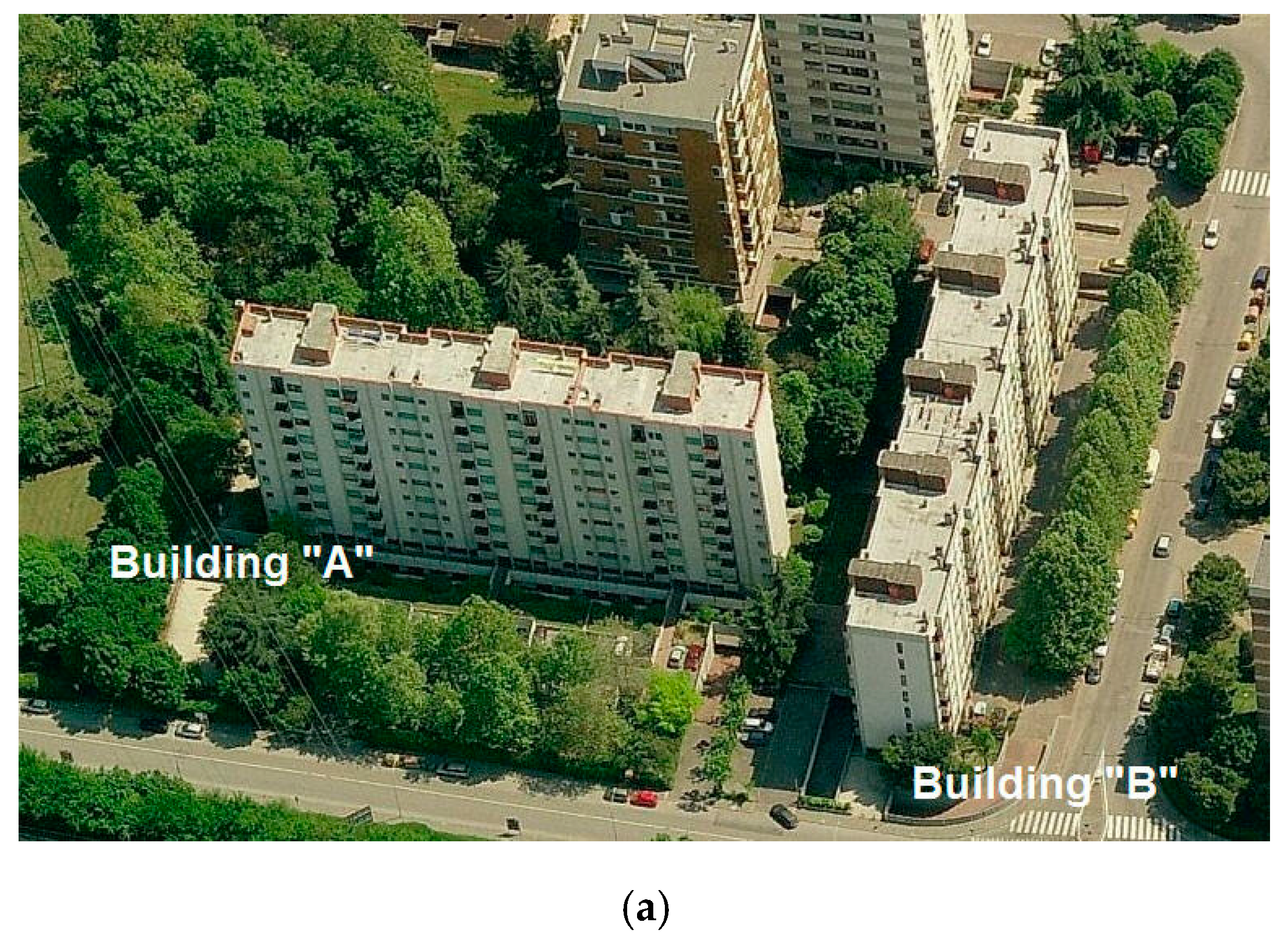
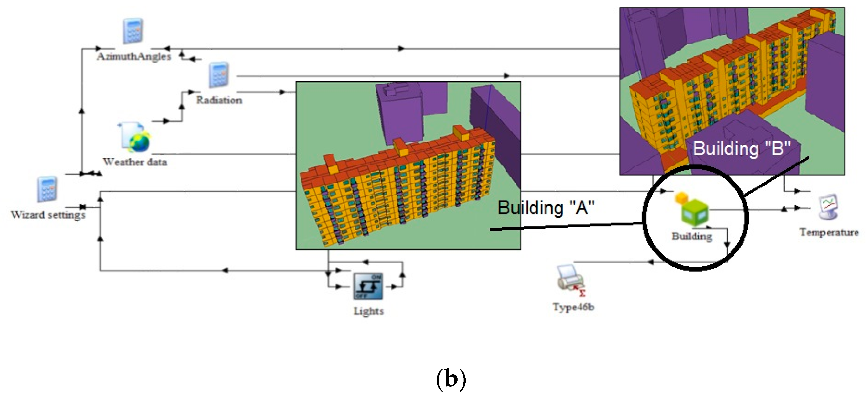
2. Description of the Example Case Study

The numerical model has been applied to a residential complex located in Bologna (Italy) and built in 1972, before the issuing in Italy of any law regarding energy saving in buildings.

The construction, depicted in Figure 1a, is made of two blocks named “building A” and “building B”, including, respectively, 54 and 72 apartments. Figure 1b provides a general overview of the domain developed in the simulations, with reference to TRNSYS ambient.

Table 1. Main dimensional characteristics of the building blocks under investigation.

Building dimensions	Building A	Building B
Building dimensions [m] (length × width × height)	67.8 × 11.3 × 33.6	95.4 × 10.4 × 24.3
Net surface [m2]	5292	5833
Average net surface per apartment [m2]	98	81
Net heated volume [m3]	14,818	16,332

highlights the main dimensional characteristics of the above-mentioned building blocks.

Table 2. Values of the thermal transmittance referred to the envelope elements (before retrofitting) and description of the materials forming the envelope.

Building Component	Layers	Thickness [m]	Heat Transfer Coefficient U [Wm−2K−1]
External walls	Concrete panel	0.290	1.95
	Gypsum plasterboard	0.015
Internal floors	Ceramic tiles	0.010	1.65
	Lightweight concrete slab	0.020
	Reinforced concrete slab	0.040
	Masonry blocks	0.180
	Gypsum plasterboard	0.015
Roof	Roof covering	0.010	1.47
	Low-slope concrete slab	0.060
	Reinforced concrete slab	0.050
	Masonry blocks	0.180
	Gypsum plasterboard	0.015
Internal walls (between apartments)	Gypsum plasterboard	0.015	1.25
	Masonry block	0.150
	Gypsum plasterboard	0.015
Windows single-pane	Clear glass pane	0.004	5.67

illustrates the thermal characteristics of the building envelope.

The heating system of the entire residential complex is located in the farthest portion of building A. It is composed by the following fundamental components: A boiler powered by natural gas as a generation subsystem, a network of pipes as a distribution subsystem, and radiators as an emission subsystem. It is supposed to operate 14 h per day, precisely 6–9 a.m., 11 a.m.–2 p.m., and 3–11 p.m. In those periods, it is set to maintain the internal prescribed temperature of 20 °C.

In the present study, the energy performance of the reference case has been investigated, i.e., the pre-retrofitting condition (named Scenario 0), and of other three retrofitting scenarios (Scenarios 1, 2, and 3) that correspond respectively to windows replacement, external walls additional insulation, and simultaneously the retrofit solutions including both high efficiency windows and improved thermal envelope (both external walls and roofing). Trnsys simulations were performed, by means of the TrnBuild package, with a time step of 1 h, dividing all the building complex under investigation into the following zones: 486 zones in building A and 432 zones in building B. We mainly utilized the standard Trnsys library, Type 56, the Building model [18]. This component describes a simplified method for providing heating and cooling equipment. Building model in Type 56 is essentially an energy balance method in which the heat flux (due to conduction and convection) to the air node is described as follows:

$${\stackrel{.}{Q}}_i={\stackrel{.}{Q}}_{surf,i}+{\stackrel{.}{Q}}_{\inf ,i}+{\stackrel{.}{Q}}_{vent}+{\stackrel{.}{Q}}_{g,c,i}+{\stackrel{.}{Q}}_{cp\lg ,i}$$

(1)

where ${\stackrel{.}{Q}}_i$ is the conductive and convective heat flux, ${\stackrel{.}{Q}}_{surf,i}$ is the surface heat gains (convection from outdoor temperature), ${\stackrel{.}{Q}}_{\inf ,i}$ is the infiltration gains, ${\stackrel{.}{Q}}_{vent}$ is the ventilations gains, ${\stackrel{.}{Q}}_{g,c,i}$ is the internal gains such as radiators, people, computers used in the room etc., and ${\stackrel{.}{Q}}_{cp\lg ,i}$ represents the gains due to convective air flow from adjacent zones. Radiative heat flows to the walls and windows are contemplated in the following equation balance:

$${\stackrel{.}{Q}}_{r,wi}={\stackrel{.}{Q}}_{g,r,i,wi}+{\stackrel{.}{Q}}_{sol,wi}+{\stackrel{.}{Q}}_{long,wi}+{\stackrel{.}{Q}}_{wall-gain}$$

(2)

where ${\stackrel{.}{Q}}_{r,wi}$ represents the radiative gains for the wall surface temperature node, ${\stackrel{.}{Q}}_{g,r,i,wi}$ the radiative air node internal gains received by walls, ${\stackrel{.}{Q}}_{sol,wi}$ the solar gains through windows received by walls, ${\stackrel{.}{Q}}_{long,wi}$ the long wave radiation exchange between a wall and all the other walls and windows, and ${\stackrel{.}{Q}}_{wall-gain}$ is the user specified heat flow to the wall or window surface. All the quantities reported in Equations (1) and (2) are given in the unit kJ/hr. In Type 56, the long wave radiation between the inner surfaces of walls and windows is also taken into account:

$$G_{ir}={\left(I-F{\rho }_{ir}\right)}^{-1}F{\epsilon }_{ir}$$

(3)

where ${\rho }_{ir}$ and ${\epsilon }_{ir}$ are diagonal matrices describing reflectivity and emissivity, respectively. The variable I corresponds to the identity matrix, and F represents the view factor, i.e., the fraction of diffusively radiated energy leaving from a generic surface A that collides with the surface B. The weather data (such as external temperature, solar radiation, etc.) are deducted from Meteonorm, as well as the solar gains that are calculated by means of Trnsys from the input of the Meteonorm file [18].

Table 3. Monthly data referred to the mean temperatures of external air in Bologna.

Month	External Air Mean Temperature (°C)
October (15 days)	12.4
November	8.4
December	3.9
January	1.7
February	4.3
March	9.4
April (15 days)	15.0

highlights the data with mean values of the external air temperatures referred to the locality of Bologna (Italy), having 2383-degree days:

All the cases under investigation are referred to the period when the heating system is switched on (winter period), which is for Bologna from 15 October to 15 April, as indicated by the Italian law [23].

3. Simulations Results

The following paragraphs are dedicated to illustrating the simulations results, subdividing them for clarity into four categories: (i) Pre-retrofitting condition, (ii) high efficiency windows, (iii) external walls additional insulation, and (iv) high efficiency windows, external walls and roofing additional insulation. All the results referred to each retrofitting scenario will be compared with the primary energy data of the pre-retrofitting condition in order to quantify the energy savings margins.

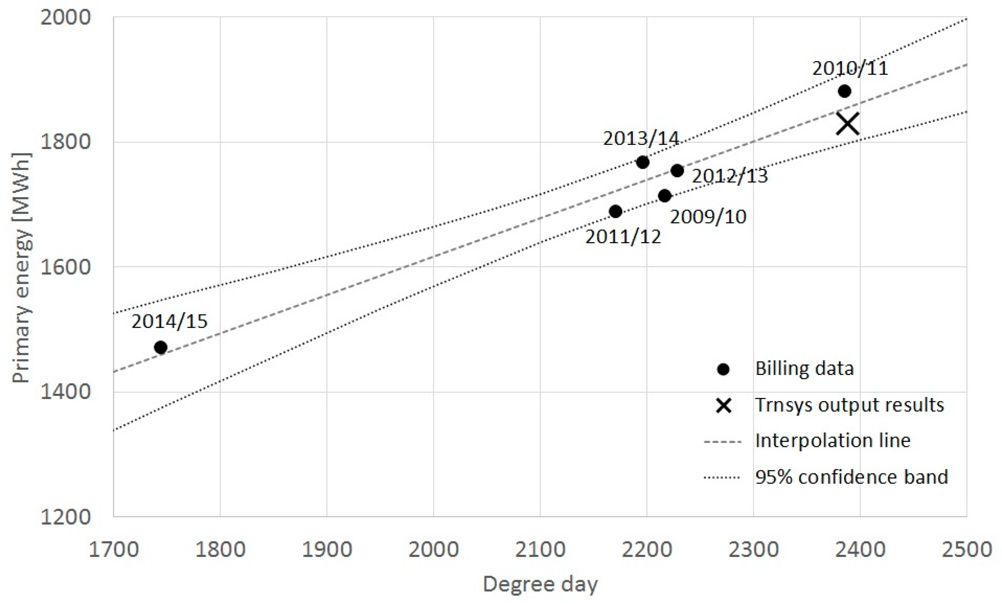
3.1. Scenario 0: Pre-Retrofitting Condition

The building envelope is firstly considered in the actual state, before the above-mentioned retrofit actions of windows replacement and thermal improvement of the envelope. The numerical code adopted here has been calibrated by comparison with the utility billing data, precisely natural gas consumption data, keeping into account all heating systems effectiveness indicators, i.e., generation efficiency (η_gn = 0.92), distribution efficiency (η_dis = 0.82), and emission and control in room spaces efficiency (η_en = 0.90). Emission and control efficiency index, as well as distribution efficiency term, have been taken from the standard UNI EN 15316: 2008 [24]. It is worthwhile to mention that the generation efficiency value has been directly determined from the in-situ measurements that have to be performed annually according to the Italian regulation [25].

On the basis of the above-mentioned hypotheses, the global heating system efficiency with reference to the case here investigated (given by the algebraic product of all efficiency terms) resulted to be approximately equal to 0.68. Thus, from this point on in the present investigation, all the output results coming from TRNSYS simulations have been converted into primary energy data dividing the energy need by the above-mentioned overall heating system efficiency.

In order to calibrate the numerical model by means of comparison with the billing data, the ideal approach is to set up a database containing as much energy use and climate data as possible: This procedure has been named in literature “inverse modeling” [26], in opposition to the “forward modeling”, in which energy predictions are assembled on the basis of physical properties of building systems, including geometry, location, and envelope.

The dataset used in this study contains utility billing data referred to natural gas consumption from 2009 to 2015: This temporal range proved to be fully exhaustive to capture the energy performance of the residential complex under investigation. Figure 2 highlights the comparison between billing data (given by the regression line) and Trnsys output results: In correspondence to the abscissa value of 2383-degree days, which is the calculated value from Meteonorm referred to the locality of Bologna, the primary energy consumption given by billing data is equal to 1853.8 MWh, and the one estimated by numerical investigation is 1832.9 MWh. The two sets of results agree within 1.1%.

Considering the global heating system efficiency equal to 0.68, the monthly and yearly energy demand can be highlighted in terms of primary energy, as reported in

Table 4. Monthly and total energy demand of the considered residential complex (Building A and Building B) with reference to the pre-retrofitting condition.

Month	Energy Demand, Building A, Q [kWh]	Energy Demand, Building B, Q [kWh]
October (15 days)	33,772	54,946
November	111,870	146,878
December	179,374	223,483
January	194,746	242,266
February	149,945	187,964
March	90,981	122,599
April (15 days)	36,147	57,909
TOTAL	796,834	1,036,045

.

Table 5. Primary energy demand of the considered residential complex (Building A and Building B) subdivided by floor in the pre-retrofitting condition.

Floor	Energy Demand, Building A, Q [kWh]	Energy Demand, Building B, Q [kWh]
Floor 1	85,847	23,799
Floor 2	91,364	141,272
Floor 3	76,173	152,239
Floor 4	80,949	159,423
Floor 5	88,005	133,947
Floor 6	75,536	144,666
Floor 7	80,792	124,227
Floor 8	84,009	156,472
Floor 9	134,159	-
TOTAL	796,834	1,036,045

shows the primary energy need floor by floor in the pre-retrofitting scenario of the building blocks under investigation: This procedure is aimed to promote a comparison with energy data after retrofitting, to see which parts of the building complex will be particularly affected by the retrofit actions in terms of energy saving.

3.2. Scenario 1: High Efficiency Windows

The first requalification action consists in including high efficiency windows: The total thermal transmittance (frame and glazing) is assumed to be equal to 1.37 Wm⁻²K⁻¹, the corresponding U-value before retrofit being 5.67 Wm⁻²K⁻¹ (see Table 2).

A questionnaire was administrated to residents for each apartment in order to describe the objective and subjective conditions; thus, it has been established that in some of the housing units (precisely 18 apartments in Building A and 14 in Building B) the “original” windows (dated 1972) had already been substituted in favor of more recent ones, having double pane glass and total thermal transmittance (on average) equal to 2.83 Wm⁻²K⁻¹. Based on the above-mentioned considerations, a great energy saving amount in Scenario 1 is not expected. Therefore, even the economic issues referred to Scenario 1, treated in next section, will be strongly affected by this “partial” requalification action.

The simulations result in terms of primary energy need (keeping the system efficiency equal to 0.68) for building heating in the considered time interval (from 15 October to 15 April) are shown in

Table 6. Primary energy demand of the considered residential complex (Building A and Building B) subdivided by floor with reference to the first retrofitting condition.

Floor	Energy Demand, Building A, Q [kWh]	Energy Demand, Building B, Q [kWh]
Floor 1	75,076	17,791
Floor 2	77,913	116,647
Floor 3	70,119	125,498
Floor 4	74,894	132,619
Floor 5	79,551	114,968
Floor 6	69,900	116,303
Floor 7	74,656	108,347
Floor 8	75,026	134,656
Floor 9	125,945	-
TOTAL	723,080	866,829

, with reference to the energy demand of each building floor.

The total amount of energy saving (Building A and Building B), with reference to the current retrofit action (high efficiency windows), obtained by comparison with the data highlighted in Table 5, i.e., the pre-retrofitting condition, results to be 243.0 MWh.

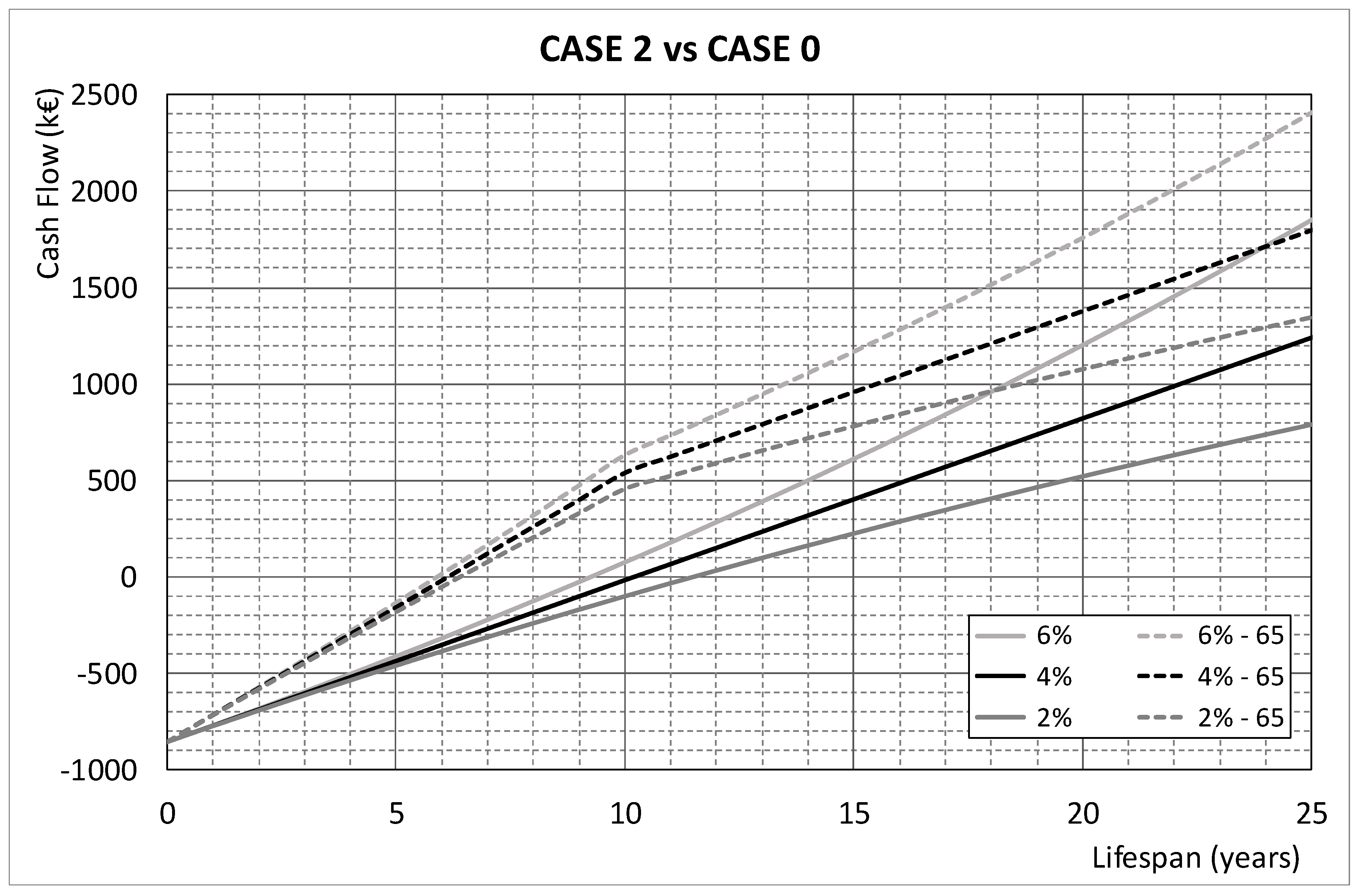
3.3. Scenario 2: External Walls Additional Insulation

The second retrofit action considers additional insulation on the external walls by adding an external layer of polystyrene (thermal conductivity: 0.03 Wm⁻¹K⁻¹; thickness: 0.16 m). The thermal transmittance is now equal to 0.17 Wm⁻²K⁻¹, the corresponding U-value before retrofit being 1.95 Wm⁻²K⁻¹ (see Table 2). The simulation results in terms of primary energy need (keeping the system efficiency still equal to 0.68) for building heating in the considered time interval (from 15 October to 15 April) are shown in

Table 7. Primary energy demand of the considered residential complex (Building A and Building B) subdivided by floor, with reference to Scenario 2.

Floor	Energy Demand, Building A, Q [kWh]	Energy Demand, Building B, Q [kWh]
Floor 1	39,347	21,793
Floor 2	36,755	80,360
Floor 3	29,737	82,452
Floor 4	30,238	88,639
Floor 5	32,908	65,487
Floor 6	27,580	79,038
Floor 7	25,303	62,510
Floor 8	35,017	78,812
Floor 9	86,474	-
TOTAL	343,359	559,091

, with reference to the energy demand of each building floor.

Similarly, the total amount of energy saving (Building A and Building B), with reference to the current retrofit action (external wall additional insulation), obtained by comparison with the data highlighted in Table 5, i.e., the pre-retrofitting condition, results to be 930.4 MWh.

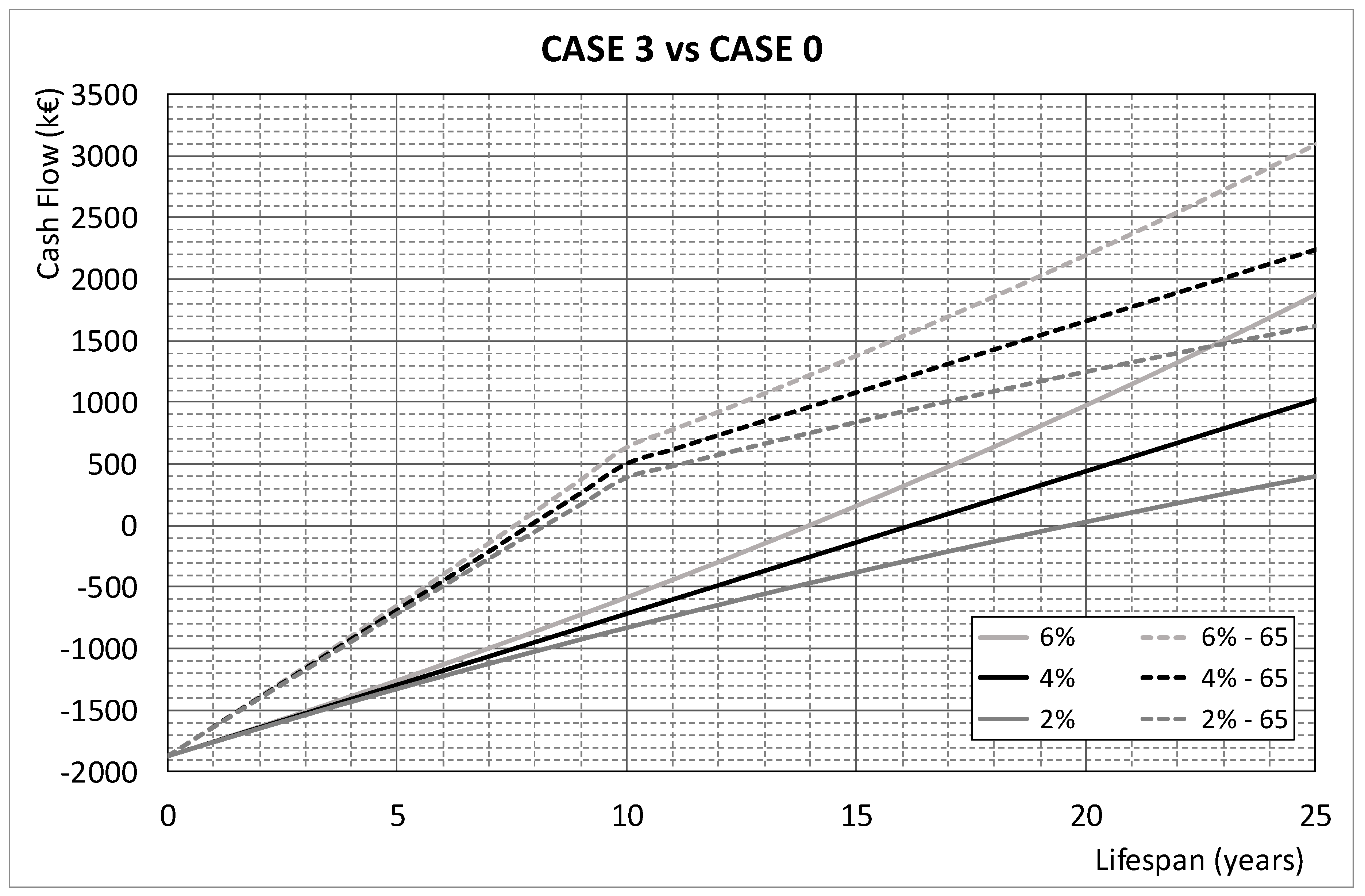
3.4. Scenario 3: High Efficiency Windows, External Walls, and Roofing Additional Insulation

Case 3 contemplates the simultaneous retrofitting of high efficiency windows and external walls additional insulation (already treated separately in Scenarios 1 and 2) with the addition of supplementary insulation of the roofing. Thermal transmittance data of windows and external walls have already been highlighted in the previous sections; the thermal transmittance of roofing is now assumed equal to 0.17 Wm⁻²K⁻¹, the corresponding U-value before retrofit being 1.47 Wm⁻²K⁻¹ (see Table 2). In the same way, the simulation results in terms of primary energy need (keeping the system efficiency still equal to 0.68) for building heating in the considered time interval (from 15 October to 15 April) are shown in

Table 8. Primary energy demand of the considered residential complex (Building A and Building B) subdivided by floor, with reference to Scenario 3.

Floor	Energy Demand, Building A, Q [kWh]	Energy Demand, Building B, Q [kWh]
Floor 1	28,501	16,255
Floor 2	22,672	46,597
Floor 3	21,262	46,610
Floor 4	21,794	51,346
Floor 5	21,729	37,250
Floor 6	20,734	43,079
Floor 7	21,717	44,880
Floor 8	18,534	56,851
Floor 9	25,709	-
TOTAL	202,652	342,868

, with reference to the energy demand of each building floor.

The total amount of energy saving (Building A and Building B), with reference to the current retrofit action (high efficiency windows in addition with external wall and roofing additional insulation), obtained by comparison with the data reported in Table 5, i.e., the pre-retrofitting condition, results to be equal to 1287.4 MWh.

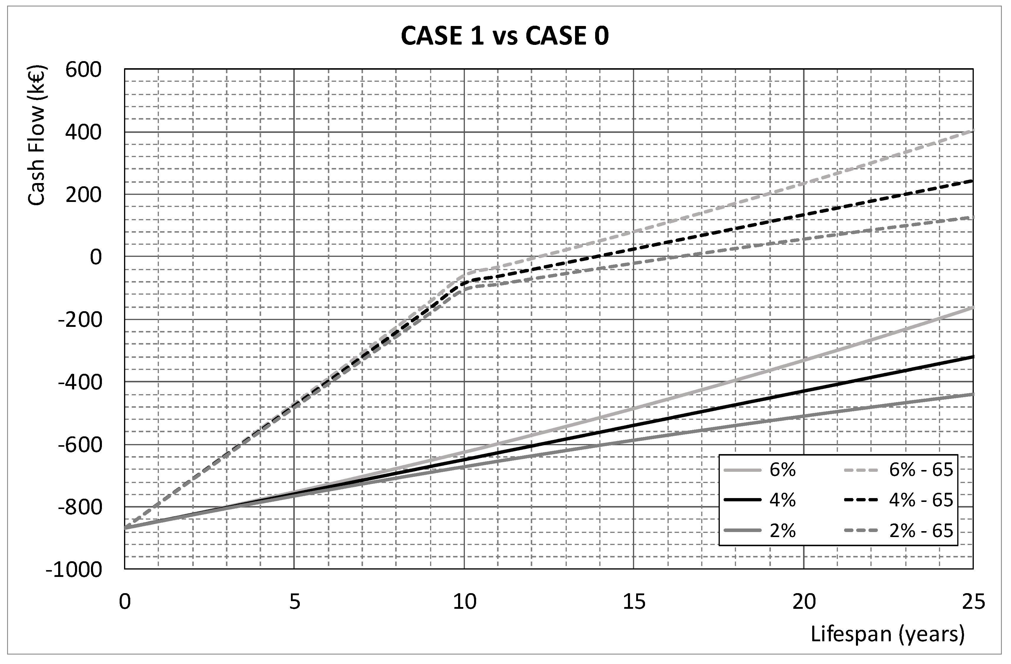
4. Economic Assessment

The economic performance associated with the above-mentioned retrofitting actions were estimated both in terms of Payback Time (PBT) and Net Present Value (NPV):

$$PBT=\frac{I_0}{S}$$

(4)

$$NPV=-I_0+{\displaystyle {\sum }_{n=1}^{LS}\frac{S_n-C_n}{{\left(1+r\right)}^n}}$$

(5)

$$S_n=S{\left(1+i\right)}^n$$

(6)

where:

−

I₀ is the initial investment cost of the project,

−

S is the energy saving evaluated at year 0,

−

S_n is the energy saving for year n,

−

C_n is the maintenance cost for year n,

−

n is the time period,

−

LS is the lifespan,

−

r is the discount rate of investment, and

−

i is the yearly increment of the cost of energy.

The investment cost analysis, with reference to the retrofitting cases under investigation, has been performed according to the above-mentioned different scenarios and the technical-economic condition in Italy was referred to the year 2017. The operating costs were evaluated with reference to the Italian scenario by assuming the unit cost of natural gas equal to 0.09 €/kWh [27].

Table 9. Initial investment and energy saving during the first year referred to all the retrofitting scenarios.

Cost analysis	Scenario 1	Scenario 2	Scenario 3
Investment [€]	867,643	855,110	1,871,912
Energy cost saving [€]	21,867	83,739	115,862

highlights the initial investment and the energy saving obtained during the first year since the retrofitting. Please note that the investment cost is intended as the global cost of each intervention, accounting both material and labor.

NPV is calculated for each scenario by taking into account a discount rate of investment of 4% and different increments of the cost of energy (2%, 4%, or 6%) according to Ref. [28]. In the present evaluation, a lifespan of 25 years is considered with reference to all the retrofitting actions. According to the Italian regulation on energy saving in the building sector, it is possible to claim a tax refund of 65% of the investment cost in 10 years [23]. NPV and SPBT have been calculated numerically either without tax refund claim or considering a 65% tax refund in 10 years. Those values, with reference to each different scenario, are reported in

Table 10. Net Present Value (lifespan 25 years) and Payback Time calculated for Scenario 1 (Case 1 vs. Case 0) at different increments of the cost of energy, (i), considering or not considering the tax refund of 65%.

Scenario 1	i = 2%	i = 4%	i = 6%
NPV (0) [k€]	−439	−321	−161
NPV (0) [k€]	125	243	403
SBT (0) [years]	78	40	30
SBT (65) [years]	16	14	12

,

Table 11. Net Present Value (lifespan 25 years) and Payback Time calculated for Scenario 2 (Case 2 vs. Case 0) at different increment of the cost of energy, (i), considering or not considering the tax refund of 65%.

Scenario 2	i = 2%	i = 4%	i = 6%
NPV (0) [k€]	787	1238	1852
NPV (0) [k€]	1343	1794	2408
SBT (0) [years]	11.5	10	9.5
SBT (65) [years]	6.5	6	6

and

Table 12. Net Present Value (lifespan 25 years) and Payback Time calculated for Scenario 3 (Case 3 vs. Case 0) at different increment of the cost of energy, (i), considering or not considering the tax refund of 65%.

Scenario 3	i = 2%	i = 4%	i = 6%
NPV (0) [k€]	401	1025	1874
NPV (0) [k€]	1617	2241	3090
SBT (0) [years]	19.5	16	14
SBT (65) [years]	8	8	7.5

.

Figure 3, Figure 4 and Figure 5 represent graphically the variation of Net Present Value during the 25 years, with reference, respectively, to Scenario 1–3.

Based on pure observation, each figure of the upper part of the diagram (in which tax refund of 65% has been contemplated) shows the change of the slope at year 10, caused by the end of the tax refund period itself. As anticipated in Section 3, Scenario 1 cannot be profitable both in terms of energy saving and consequently of payback time: The SPBT value equal to 78 years without tax refund (for i = 2%) is purely “theoretical and academic”. The reason is that high efficiency windows action was forcibly partial since it has been established that in some of the housing units (precisely 18 apartments in Building A and 14 in Building B) the “original” windows of 1972 had already been substituted in favor of more recent ones, having double pane glass and total thermal transmittance (on average) equal to 2.83 Wm⁻²K⁻¹. Therefore, this fact also affected Scenario 3, in which all the actions of high efficiency windows, external walls and roofing additional insulation have been contemplated simultaneously. Thus, Scenario 2 resulted to be the most profitable solution, with an optimal SPBT of roughly 6 years with tax refund. Finally, it is worth mentioning that all the above-mentioned observations are fully supported by the values shown in Table 10, Table 11 and Table 12 and Figure 3, Figure 4 and Figure 5.

Sensitivity Analysis

The results of the previous paragraph are related to assumptions on a set of input variables. Since the cost of energy and the cost of capital are critical variables, a sensitivity analysis based on the same procedure illustrated in Ref. [17] has been performed. The variation of both price of natural gas and discount rate of the investment has been contemplated.

Annual natural gas purchase price (gpc) evaluates the variation of energy cost reported in energy invoices. A pessimistic scenario is associated with a reduction in supply energy price, whilst the scenario is optimistic when the gpc is increasing. The base case considers the selling price of natural gas of 9 c€. Two negative scenarios (selling price of 7 and 8 c€) and two positives (selling price of 10 and 11 c€) have been analyzed in terms of variation of NPV. The discount rate of the investment is the interest rate applied by commercial banks and represents the capital cost. If compared to the base case (r = 4%), four scenarios have been analyzed: Two optimistic (r = 1% and r = 3%) and two pessimistic (r = 5% and r = 7%). The decreasing of capital cost leads to a positive investments profitability, whilst the increasing is a negative situation.

Table 13. Net Present Value and annual gas purchase price (gpc).

Case X vs. Case 0	gpc = 7 c€		gpc = 8 c€		gpc = 10 c€		gpc = 11 c€
	NPV	%	NPV	%	NPV	%	NPV	%
Case 1 vs. Case 0
NPV (65) − i = 2%	30	−76%	78	−38%	173	38%	221	76%
NPV (65) − i = 4%	122	−50%	182	−25%	304	25%	364	50%
NPV (65) − i = 6%	246	−39%	325	−19%	482	19%	560	39%
Case 2 vs. Case 0
NPV (0) − i = 2%	422	−46%	605	−23%	970	23%	1152	46%
NPV (0) − i = 4%	773	−38%	1006	−19%	1471	19%	1704	38%
NPV (0) − i = 6%	1250	−32%	1551	−16%	2153	16%	2454	32%
NPV (65) − i = 2%	978	−27%	1161	−14%	1526	14%	1708	27%
NPV (65) − i = 4%	1329	−26%	1562	−13%	2027	13%	2259	26%
NPV (65) − i = 6%	1806	−25%	2107	−12%	2709	12%	3009	25%
Case 3 vs. Case 0
NPV (0) − i = 2%	−104	−126%	148	−63%	653	63%	906	126%
NPV (0) − i = 4%	381	−63%	703	−31%	1346	31%	1668	63%
NPV (0) − i = 6%	1041	−44%	1457	−22%	2290	22%	2706	44%
NPV (65) − i = 2%	1112	−31%	1365	−16%	1870	16%	2122	31%
NPV (65) − i = 4%	1598	−29%	1920	−14%	2563	14%	2885	29%
NPV (65) − i = 6%	2258	−27%	2674	−13%	3507	13%	3923	27%

shows the NPV and the percentage variation related to the base case for different values of the annual gas purchase price.

It is worthwhile to mention that in the scenario named “Case 1 vs. Case 0”, the output results referred to negative values of NPV have not been reported. Based on pure observations, the values highlighted in Table 13 seem to delineate a linear relationship between gpc and NPV.

Table 14. Net Present Value and discount rate of the investment.

Case X vs. Case 0	r = 1%		r = 3%		r = 5%		r = 7%
	NPV	%	NPV	%	NPV	%	NPV	%
Case 1 vs. Case 0
NPV (65) − i = 2%	319	155%	179	43%	80	−36%	8	−94%
NPV (65) − i = 4%	514	112%	318	31%	180	−26%	82	−66%
NPV (65) − i = 6%	784	94%	507	26%	316	−22%	181	−55%
Case 2 vs. Case 0
NPV (0) − i = 2%	1530	94%	994	26%	613	−22%	337	−57%
NPV (0) − i = 4%	2276	84%	1524	23%	998	−19%	622	−50%
NPV (0) − i = 6%	3311	79%	2251	22%	1518	−18%	1002	−46%
NPV (65) − i = 2%	2086	55%	1549	15%	1168	−13%	893	−34%
NPV (65) − i = 4%	2832	58%	2080	16%	1554	−13%	1178	−34%
NPV (65) − i = 6%	3867	61%	2807	17%	2074	−14%	1558	−35%
Case 3 vs. Case 0
NPV (0) − i = 2%	1429	257%	686	71%	159	−60%	−223	−156%
NPV (0) − i = 4%	2461	140%	1420	39%	692	−32%	172	−83%
NPV (0) − i = 6%	3892	108%	2426	29%	1412	−25%	698	−63%
NPV (65) − i = 2%	2646	64%	1903	18%	1376	−15%	994	−39%
NPV (65) − i = 4%	3678	64%	2637	18%	1909	−15%	1389	−38%
NPV (65) − i = 6%	5109	65%	3643	18%	2629	−15%	1914	−38%

illustrates the NPV and the percentage variation related to the base case for different values of the discount rate of the investments.

In general, the sensibility analysis has confirmed the results exposed in paragraph 4, showing weak variations, especially when the fiscal incentives are contemplated. The only exception in this sense can be represented by Case 3.

5. Conclusions

This paper deals with an integrated passive design approach to reduce the heating demand for an existing residential complex located in Bologna, in the northern part of Italy. These measures are high efficiency windows, external walls additional insulation, and simultaneously the retrofit solutions of high efficiency windows and improved thermal envelope, both on external walls and roofing. The numerical model, here developed in the Trnsys ambient, has been calibrated by means of the real consumption data deduced from energy bills (years 2009–2015), in coherence with the procedure adopted in Ref. [29]. Scenario 1 proved to be the worst case both in terms of energy saving and consequently of payback time. The reason is that the high efficiency windows action here developed was forcibly partial since it has been established that in some of the housing units the “original” windows of 1972 had already been substituted in favor of more recent ones, having double pane glasses. Therefore, this fact also affected Scenario 3, in which all the actions of high efficiency windows and external walls and roofing additional insulation have been contemplated simultaneously. Thus, Scenario 2 proved to be the most profitable solution: The calculated total amount of energy saving (Building A and Building B), obtained by comparison with the pre-retrofitting condition, resulted to be equal to 930.4 MWh, with an optimal SPBT of roughly six years when tax refund is contemplated. Finally, it is worthwhile to mention that in the actual context of the cost of energy in Italy, retrofitting actions on existing residential buildings can be encouraged, provided that national policies of incentives are maintained. Future developments of the research presented here may include the adoption of Phase Change Materials (PCMs) integrated in the building structure, as an additional and innovative retrofitting solution. Among the approachable technologies, Phase Change Materials (PCMs) are substances that undergo a phase transition (in general solid-liquid) at their utilization temperature. They can store (during melting) and release (during solidification) large quantities of energy at an almost constant temperature by exploiting their latent heat of fusion. Therefore, PCMs in buildings can be utilized to augment the heat storage capacity or to obtain a stabilizing effect on temperature swings, thus reducing building energy use, diminishing peak heating and cooling loads. Finally, a further starting point for reflection on possible developments can be represented by the combined study of retrofitting actions on the thermal envelope associated with the implementation of renewable energies, such as photovoltaic panels. On this topic, interconnection with the electricity grid [30,31] will also come into play.

References

1. European Commission. Climate Action Paris Agreement. Available online: https://ec.europa.eu/clima/policies/international/negotiations/paris_en (accessed on 6 June 2018).
2. European Commission. Second Report on the State of the Energy Union; European Commission: Brussels, Belgium, 2017. [Google Scholar]
3. De Rosa, M.; Bianco, V.; Scarpa, F.; Tagliafico, L.A. Heating and cooling building energy demand evaluation: A simplified model and a modified degree days approach. Appl. Energy. 2014, 28, 217–229. [Google Scholar] [CrossRef]
4. Wang, B.; Xia, X.; Zhang, J. A multi-objective optimization model for the life-cycle cost analysis and retrofitting planning of buildings. Energy Build. 2014, 77, 227–235. [Google Scholar] [CrossRef] [Green Version]
5. Fan, Y.; Xia, X. A multi-objective optimization model for energy-efficiency building envelope retrofitting plan with rooftop PV system installation and maintenance. Appl. Energy 2017, 189, 327–335. [Google Scholar] [CrossRef]
6. Wua, R.; Mavromatidisa, G.; Orehouniga, K.; Carmelieta, J. Multiobjective optimisation of energy systems and building envelope retrofit in a residential community. Appl. Energy 2017, 190, 634–649. [Google Scholar] [CrossRef]
7. Delmastro, C.; Mutani, G.; Corgnati, S.P. A supporting method for selecting cost-optimal energy retrofit policies for residential buildings at the urban scale. Energy Policy 2016, 99, 42–56. [Google Scholar] [CrossRef]
8. BPIE. Europe’s under the Microscope; Building Performance Institute: Brussel, Belgium, 2011. [Google Scholar]
9. Mazzarella, L. Energy Retrofit of historic and existing buildings. The legislative and regulatory point of view. Energy Build. 2015, 95, 23–31. [Google Scholar] [CrossRef]
10. Mauro, G.M.; Hamdy, M.; Vanoli, G.P.; Bianco, N.; Hensen, J.L.M. A new retrofitting methodology for investigating the cost-optimality of energy retrofitting a building category. Energy Build. 2015, 107, 456–478. [Google Scholar] [CrossRef]
11. Nguyen, A.T.; Reiter, S.; Rigo, P. A review on simulation-based optimization methods applied to building performance analysis. Appl. Energy 2014, 113, 1043–1058. [Google Scholar] [CrossRef] [Green Version]
12. Ascione, F.; Bianco, N.; De Stasio, C.; Mauro, G.M.; Vanoli, G.P. A new methodology for cost-optimal analysis by means of the multi-objective optimization of building energy performance. Energy Build. 2015, 88, 78–90. [Google Scholar] [CrossRef]
13. Penna, P.; Prada, A.; Cappelletti, F.; Gasparella, A. Multi-objectives optimization of energy efficiency measures in existing buildings. Energy Build. 2015, 95, 57–69. [Google Scholar] [CrossRef]
14. Marrone, P.; Gori, P.; Asdrubali, F.; Evangelisti, L.; Calcagnini, L.; Grazieschi, G. Energy Benchmarking in Educational Buildings through Cluster Analysis of Energy Retrofitting. Energies 2018, 11, 649. [Google Scholar] [CrossRef]
15. Moschetti, R.; Brattebo, H. Combining Life Cycle Environmental and Economic Assessments in Building Energy Renovation Projects. Energies 2017, 10, 1851. [Google Scholar] [CrossRef]
16. Choi, B.-E.; Shin, J.-H.; Lee, J.-H.; Kim, S.-S.; Cho, Y.-H. Development of Decision Support Process for Building Energy Conservation Measures and Economic Analysis. Energies 2017, 10, 324. [Google Scholar] [CrossRef]
17. Cucchiella, F.; D’Adamo, I.; Gastaldi, M. Economic Analysis of a Photovoltaic System: A Resource for Residential Households. Energies 2017, 10, 814. [Google Scholar] [CrossRef]
18. Klein, S.A.; Beckman, W.A.; Mitchell, J.W.; Duffie, J.A.; Duffie, N.A.; Freeman, T.L.; Mitchell, J.C.; Braun, J.E.; Evans, B.L.; Kummer, J.P.; et al. TRNSYS Version. 17; Solar Energy Laboratory, University of Wisconsin-Madison: Madison, WI, USA, 2010. [Google Scholar]
19. Paudel, S.; Elmitri, M.; Couturier, S.; Nguyen, P.H.; Kamphuis, R.; Lacarrière, B.; Le Corre, O. A relevant data selection method for energy consumption prediction of low energy building based on support vector machine. Energy Build. 2017, 138, 240–256. [Google Scholar] [CrossRef]
20. Inanici, M.N.; Demirbilek, F.N. Thermal performance optimization of building aspect ratio and south window size in five cities having different climatic characteristics of Turkey. Build. Environ. 2000, 35, 41–52. [Google Scholar] [CrossRef]
21. Persson, M.L.; Roos, A.; Wall, M. Influence of window size on the energy balance of low energy houses. Energy Build. 2006, 38, 181–188. [Google Scholar] [CrossRef]
22. Skarning, G.C.J.; Hviid, C.A.; Svendsen, S. Roadmap for improving roof and façade windows in nearly zero-energy houses in Europe. Energy Build. 2016, 116, 602–613. [Google Scholar] [CrossRef] [Green Version]
23. Legge Finanziaria n. 296/2006 and Legge di Stabilità n. 208/2015. Available online: http://www.bosettiegatti.eu/info/norme/statali/2015_0208_stabilita.htm (accessed on 28 June 2018).
24. Heating Systems in Buildings—Method for Calculation of System Energy Requirements and System Efficiencies; UNI EN 15316-2-1:2008; Uni, Ente Italiano di Normazione: Milan, Italy, 2008.
25. Regolamento Recante Norme per la Progettazione, l’installazione, l’esercizio e la Manutenzione Degli Impianti Termici Degli Edifici ai Fini Del Contenimento dei Consumi di Energia, in Attuazione dell’art. 4, Comma 4, Della L. 9 Gennaio 1991, n. 10; D.P.R. 26 Agosto 1993, n. 412; Gazzetta Ufficiale, Istituto Poligrafico e Zecca dello Stato: Rome, Italy, 1993.
26. Park, J.S.; Lee, S.J.; Kim, K.H.; Kwon, K.W.; Jeong, J.-M. Estimating thermal performance and energy saving potential of residential buildings using energy bills. Energy Build. 2016, 110, 23–30. [Google Scholar] [CrossRef]
27. Aste, N.; Caputo, C.; Buzzetti, M.; Fattore, M. Energy efficiency in buildings: What drives the investments? The case of Lombardy Region. Sustain. Cities Soc. 2016, 20, 27–37. [Google Scholar] [CrossRef]
28. Valdiserri, P.; Biserni, C. Energy performance of an existing office building in the northern part of Italy: Retrofitting actions and economic assessment. Sustain. Cities Soc. 2016, 27, 65–72. [Google Scholar] [CrossRef]
29. Allesina, G.; Musatti, E.; Ferrari, F.; Muscio, A. A calibration methodology for building dynamic models based on data collected through survey and billings. Energy Build. 2018, 158, 406–416. [Google Scholar] [CrossRef]
30. Bahrami, S.; Amini, M.H.; Shafie-khah, M.; Catalao, J.P.S. A Decentralized Electricity Market Scheme Enabling Demand Response Deployment. IEEE Trans. Power Syst. 2017, 33, 4218–4227. [Google Scholar] [CrossRef]
31. Mohammadi, A.; Dehghani, M.J.; Ghazizadeh, E. Game Theoretic Spectrum Allocation in Femtocell Networks for Smart Electric Distribution Grids. Energies 2018, 11, 1635. [Google Scholar] [CrossRef]
Figure 1. (a) Photograph of the residential complex under investigation. (b) Schematic overview of the computational domain.
Energies 11 02055 g001aEnergies 11 02055 g001b
Figure 2. Calibration of the numerical code: Comparison between billing data and simulations results.
Energies 11 02055 g002
Figure 3. Cash flows referred to Scenario 1, at different increments of the cost of energy, (i), considering or not considering the tax refund of 65%—lifespan 25 years.
Energies 11 02055 g003
Figure 4. Cash flows referred to Scenario 2, at different increment of the cost of energy, (i), considering or not considering the tax refund of 65%—lifespan 25 years.
Energies 11 02055 g004
Figure 5. Cash flows referred to Scenario 3, at different increment of the cost of energy, (i), considering or not considering the tax refund of 65%—lifespan 25 years.
Energies 11 02055 g005