Methodology and Continuous Time Mathematical Model to Select Optimum Power of Gas Turbine Set for Dual-Fuel Gas-Steam Combined Heat and Power Plant in Parallel System

Abstract

This paper contains the results of a study in which a novel approach using continuous time notation was applied in the search for the optimum capacity of a gas turbine designed for a dual-fuel gas-steam combined heat and power plant in a parallel system. As a result of the application of mathematical models of any functions that account for variations in time of all integrand quantities, for example prices of energy carriers, the model that was developed provides a way to analyze complex dependencies. The results of calculations obtained as a result of using this notation provide a rational selection of technologies and equipment designed for the energy industry. The results are based on an analysis involving a combined heat and power plant with an extraction-condensing steam turbine and extraction backpressure steam turbine for a wide range of the variability in energy prices and environmental charges corresponding to the current prices and environmental charges. All the curves were obtained using innovative methodology and mathematical model in which the total, discounted profit is calculated at the given moment and expressed as NPV achieved from the operation of dual-fuel gas-steam combined heat and power (CHP) plant.

1. Introduction

Coal resources in the world, and also in Poland, are huge and we can forecast that energy sector can use it for many years to come. To use the resources in a rational way from the point of view of technology, the combustion of coal should apply so-called clean technology. Dual-fuel gas-steam technology forms an example, as the Joule gas turbine cycle is coupled with the Clausius–Rankine cycle of a steam turbine in a parallel or serial system in it [1,2,3]. Moreover, when coal combustion in dual-fuel gas-steam systems takes place with the simultaneous production of electricity and useful heat, for example to cater meet the demands of municipal heating, this will additionally lead to a significant reduction in global coal consumption resulting in a decrease of the emission of harmful combustion products into the environment. Therefore, it is necessary to conduct a technical and economic analysis of the combined production of electricity and heat in dual-fuel gas-steam systems to determine the economic feasibility of using them. In this work, a newly commissioned combined heat and power (CHP) plant was analyzed—Figure 1. At the same time, it should be noted that the parallel system also offers a rational way to modernize existing coal-fired power stations (and power plants) for dual-fuel systems, while the serial system (Hot Windbox) is an economically feasible system designed exclusively for use in newly commissioned combined heat and power plants (and power plants).

In the literature in this area, existing reports usually focus on combined gas and steam mono-fuel systems, also so-called CCPP [2,3,4,5]. A small number of works relate to the dual-fuel gas-steam system and only deal with a few specific cases of parallel and serial connection of a gas turbine with a steam turbine [1,6,7,8,9,10,11,12,13,14,15,16,17,18]. These works only deal with selected manner in which the Joule cycle with the Clausius–Rankine cycle can be coupled, among many possible ways.

The modernization of an existing combined heat and power plant (and power plant) to the serial system (we should note that there is no recovery boiler in the serial system) would need to involve a new investment in a very expensive coal-fired boiler which is the same as for newly built combined heat and power plants (and power plants), whereas the investment in repowering to a parallel system requires a cheap heat regeneration boiler [19,20,21]. The coal boiler forms the most expensive part of the power units, both in single and dual fuel systems. It is many times more expensive than a gas turbine set, whereas the recovery boiler is about 2.5 times cheaper than a gas turbine set.

2. Methodology of Technical and Economic Analysis of Dual-Fuel Gas-Steam Systems

In a market economy, the cost-effectiveness condition of building new energy sources determines the economic feasibility by which they can operate. The economic criterion is superior to the technical one. Technical analysis, despite being very important and necessary, should be used only when the analysis is concerned with looking for opportunities to improve technology and technical processes, and when structural solutions of machines and equipment are upgraded. Ultimately, however, the economic criterion, i.e., the criterion of profit maximization, determines the purpose and selection of a specific technical solution. This paper uses the novel methodology of economic analysis of any investment projects, i.e., the methodology applying a continuous time record (Formula (1)) [22,23,24,25,26]. As a result of the possibility of using any functions that define changes in time of all integrand quantities in mathematical models, for example prices of energy carriers in the revenues S_R, the applied methodology offers the analysis of complex dependencies that would not be possible to achieve without it, or at least would be difficult to note. Therefore, the analysis presented here offers the ability to anticipate the future, and the results of calculations obtained with it offer a rational selection of energy technologies and equipment.

In continuous time notations, the total, discounted for the present NPV profit achieved by T years of operation of newly built energy installations, and not only, is expressed by the dependencies [22,23,24,25,26]:

$$NPV={\displaystyle \underset{0}{\overset{T}{\int }}\left[S_A-K_e-F-R-\left(S_A-K_e-F-A\right)p\right]{\mathrm{e}}^{-rt}}dt,$$

(1)

where:

• A—depreciation installment;
• ${\mathrm{e}}^{-rt}$—factor applied to discount money backward t = 0;
• F—time-variable interest (cost of finance) associate with financial resources spent on investment J₀; interest F forms the function of the time-variable instalments R; F = F[R(t)];
• K_e—time-variable annual exploitation cost;
• p—time-variable rate of income tax;
• R—time-variable instalments on loan repayment;
• r—time-variable discount rate;
• S_A—time-variable annual revenue;
• t—time;
• T—calculated period corresponding to operation of newly built energy installations, expressed in years.

The variable in time annual operating costs of K_e include: the cost of fuel and electricity used as the internal load K_fuel, the cost of supplementary water K_sw, the cost of wages with overheads K_sal, the cost of maintenance and overhauls K_serv, the cost of non-energy raw materials and auxiliary materials K_m, the cost for economic use of the environment K_env (including fees for emission of flue gases into the atmosphere, sewage disposal, waste storage, etc.), costs of taxes, fees and insurance K_t, cost of driving pumps network K_pum and the cost of purchasing carbon dioxide emission allowances $K_{{CO}_2}$ [22,23,24,25,26]:

$$K_e=K_{fuel}+K_{sw}+K_{sal}+K_{serv}+K_m+K_{env}+K_t+K_{{CO}_2}.$$

(2)

The cost $K_{{CO}_2}$, which comes as a result of the implementation of EU-15 climate policy by the “old” 15 EU member states, leads to a significant increase in the exploitation cost K_e of CHP [27] plants. The totals of costs $K_{sw}+K_m$ and $K_{sal}+K_t$ in Formula (2) can be taken into account by increasing, for example, a few percent, the cost of K_fuel, and a dozen or several dozen percent, the cost of K_serv.

From the Formula (1) for the condition NPV = 0, further measures of the economic efficiency of the investment are determined in a continuous time record: IRR interest rate, which invested capital J brings and expressed in terms of the years needed for its repayment (DPBP):

$${\displaystyle \underset{0}{\overset{T}{\int }}(S_A-K_e){\mathrm{e}}^{-IRRt}dt}={\displaystyle \underset{0}{\overset{T}{\int }}[F(IRR)+R(IRR)]{\mathrm{e}}^{-IRRt}dt},$$

(3)

$${\displaystyle \underset{0}{\overset{DPBP}{\int }}\left[S_A-K_e-\left(S_A-K_e-F-A\right)p\right]{\mathrm{e}}^{-rt}}dt={\displaystyle \underset{0}{\overset{T}{\int }}(F+R){\mathrm{e}}^{-rt}dt}.$$

(4)

The IRR measure (Formula (3)) according to its definition [4,5,6,7] is determined under the assumption that income tax p is equal to zero: $P=\left(S_A-K_e-F-A\right)p=0$. The records F(IRR) and R(IRR) in Formula (3) mean that the financial cost F and the installment of the loan R are functions of the IRR, whereas in Formulas (1) and (4) they are relative to the r rate with the A depreciation rate [22,23,24,25,26]. The right sides of Formulas (3) and (4) represent the discounted investment expenditure J₀ [22,23,24,25,26]:

$$J_0=zJ$$

(5)

where:

• J—turnkey investment on a CHP plant, in zloty (PLN);
• z—discounting factor (freezing ratio) investment capital J at the moment of completion of investment construction, z > 1; this coefficient takes into account the undesirable impact of the freezing of investment outlays over the construction period b, they do not bring profits during that period, while the interest on capital J increases [22,23,24,25,26]:

  $$z=\frac{{(1+r)}^{b+1}-1}{(b+1)r}.$$

  (6)

A limit is imposed on the sum of the R loan installments. It must be equal to the discounted investment expressed as J₀. The condition of constraints expressed in continuous time is given by the formula:

$${\displaystyle \underset{0}{\overset{T}{\int }}R}dt=J_0.$$

(7)

In practice, the loan repayment installment has a constant value R = const and can be calculated from Formula (7):

$$R=\frac{J_0}{T}.$$

(8)

The depreciation rate A is expressed in the same formula as the installment R. The investment J₀ depends on the applied energy technology and technical solutions.

In the general case, the evolution of the unknown function of the financial cost F = F[R(t)] describes the formula of state:

$$\frac{dF}{dt}=-rR.$$

(9)

In practice, however, the repayment installment has a fixed value R = constant and interest F is expressed by the function:

$$F(t)=r[J_0-(t-1)R].$$

(10)

As already indicated above, the value of all functions of over time in Formulas (1), (3) and (4) can be assumed for all sub-values, e.g. for any scenarios of the variable energy prices and specific rates for the emissions of pollutants into the environment [22,23,24,25,26]. Continuous time records (1), (3), (4), therefore, have an incomparable advantage over discrete records of investment effectiveness measures, which have been used in the economic analysis of economic activity so far [19,20,21]. They provide ways to analyze changes easily and quickly, such as in the search for the largest values of NPV profit.

What is more, they offer the analysis of the variability of NPV, IRR, DPBP functions and the development of their curves using differential calculus, which can provide a whole range of additional, important information that would be impossible or difficult to see without them. They can also provide an explicit assessment of the effect of individual input quantities on the final results, and above all to easily and quickly find not only the optimal solution, but also an area of solutions close to the optimal one. What is more, they allow the nature of their changes to be shown. They provide grounds for a discussion and analysis of research results. In technology, in economics, in various types of applications, this has a large and significant value. What is more, mathematical models with continuous time offer conclusions of a general nature, and only the path from the general to the detailed is correct and gives the opportunity to generalize the considerations. The way from the detailed to the general most often is not true—although that is not to say that it is usually so.

The presented notations of NPV, IRR, DPBP measures applying continuous time lead to conclusions regarding economic conditions necessary for the implementation of individual technologies and energy devices, and the most economically efficient selection [22,23,24,25,26], but also to determine economically justified price relations between energy carriers and tariffs on environmental charges. Not only that, they allow the analysis of the impact on the optimal investment strategy not only of the aforementioned relations, but also changes in their value over time.

The selection of the optimal investment strategy should be for the condition that:

NPV → max.

(11)

In the case of combined heat and power plants, the equivalent criterion for maximizing NPV profit is to minimize the unit cost of heat production in them (Formulas (19), (22) and (29)):

k_h → min.

(12)

3. Mathematical Models with Continuous Time Selection of the Optimal Power of a Gas Turbine Set for Dual-Fuel Gas-Steam Combined Heat and Power (CHP) Plants

For a combined heat and power plant both in series as well as in a parallel system, regardless of whether they comprise a steam and backpressure steam turbines or extraction-condensing steam turbines, the NPV is given by the following formula:

$$\begin{array}{cc}\hfill NPV=& [{\displaystyle \underset{0}{\overset{T}{\int }}\left(S_{el,A}+S_{Q,A}\right){\mathrm{e}}^{-rt}dt}-{\displaystyle \underset{0}{\overset{T}{\int }}{K}_e^{gas}{\mathrm{e}}^{-rt}dt}-{\displaystyle \underset{0}{\overset{T}{\int }}{K}_e^{coal}{\mathrm{e}}^{-rt}dt}+\hfill \\ & -{\displaystyle \underset{0}{\overset{T}{\int }}{K}_{e,serv}{\mathrm{e}}^{-rt}dt}-{\displaystyle \underset{0}{\overset{T}{\int }}\left(F+\frac{J_0}{T}\right)}{\mathrm{e}}^{-rt}dt](1-p)\hfill \end{array}$$

(13)

wherein the individual components in Formula (13) are expressed by the following relations:

• discounted revenues from the sales of electricity and heat

  $${\displaystyle \underset{0}{\overset{T}{\int }}\left(S_{el,A}+S_{Q,A}\right){\mathrm{e}}^{-rt}dt}=(E_{el,A}^{ST}+E_{el,A}^{GT})(1-{\epsilon }_{el})\frac{e_{el}^{t=0}}{a_{el}-r}{[\mathrm{e}}^{(a_{el}-r)T}-1]+Q_A\frac{e_h^{t=0}}{a_h-r}{[\mathrm{e}}^{(a_h-r)T}-1]$$

  (14)
• discounted operating costs related to gas (gas cost and environmental costs, excluding cost associated with maintenance, repairs, wages, taxes, insurance)

  $$\begin{array}{cc}\hfill {\displaystyle \underset{0}{\overset{T}{\int }}}{K}_e^{gas}& {\mathrm{e}}^{-rt}dt=E_{ch,A}^{gas}\{(1+x_{sw,m,was})\frac{e_{gas}^{t=0}}{a_{gas}-r}{[\mathrm{e}}^{(a_{gas}-r)T}-1]+\frac{{\rho }_{C{O}_2}^{gas}{p}_{{CO}_2}^{t=0}}{a_{C{O}_2}-r}{[\mathrm{e}}^{(a_{C{O}_2}-r)T}-1]+\hfill \\ & +\frac{{\rho }_{CO}^{gas}{p}_{CO}^{t=0}}{a_{CO}-r}[{\mathrm{e}}^{(a_{CO}-r)T}-1]+\frac{{\rho }_{N{O}_X}^{gas}{p}_{N{O}_X}^{t=0}}{a_{N{O}_X}-r}[{\mathrm{e}}^{(a_{N{O}_X}-r)T}-1]+\hfill \\ & +\frac{{\rho }_{S{O}_2}^{gas}{p}_{S{O}_2}^{t=0}}{a_{S{O}_2}-r}[{\mathrm{e}}^{(a_{S{O}_2}-r)T}-1]+\frac{{\rho }_{dust}^{gas}{p}_{dust}^{t=0}}{a_{dust}-r}[{\mathrm{e}}^{(a_{dust}-r)T}-1]+\hfill \\ & +(1-u)\frac{{\rho }_{C{O}_2}^{gas}{e}_{C{O}_2}^{t=0}}{b_{C{O}_2}-r}{[\mathrm{e}}^{(b_{C{O}_2}-r)T}-1]\}\hfill \end{array}$$

  (15)
• discounted operating costs related to coal (coal cost and environmental costs, excluding cost of maintenance, repairs, wages, taxes, insurance)

  $$\begin{array}{cc}\hfill {\displaystyle \underset{0}{\overset{T}{\int }}}{K}_e^{coal}& {\mathrm{e}}^{-rt}dt=E_{ch,A}^{coal}\{(1+x_{sw,m,was})\frac{e_{coal}^{t=0}}{a_{coal}-r}{[\mathrm{e}}^{(a_{coal}-r)T}-1]+\frac{{\rho }_{C{O}_2}^{coal}{p}_{C{O}_2}^{t=0}}{a_{C{O}_2}-r}[{\mathrm{e}}^{(a_{C{O}_2}-r)T}-1]+\hfill \\ & +\frac{{\rho }_{CO}^{coal}{p}_{CO}^{t=0}}{a_{CO}-r}[{\mathrm{e}}^{(a_{CO}-r)T}-1]+\frac{{\rho }_{N{O}_X}^{coal}{p}_{N{O}_X}^{t=0}}{a_{N{O}_X}-r}[{\mathrm{e}}^{(a_{N{O}_X}-r)T}-1]+\hfill \\ & +\frac{{\rho }_{S{O}_2}^{coal}{p}_{S{O}_2}^{t=0}}{a_{S{O}_2}-r}[{\mathrm{e}}^{(a_{S{O}_2}-r)T}-1]+\frac{{\rho }_{dust}^{coal}{p}_{dust}^{t=0}}{a_{dust}-r}[{\mathrm{e}}^{(a_{dust}-r)T}-1]+\hfill \\ & +(1-u)\frac{{\rho }_{C{O}_2}^{coal}{e}_{C{O}_2}^{t=0}}{b_{C{O}_2}-r}{[\mathrm{e}}^{(b_{C{O}_2}-r)T}-1]\}\hfill \end{array}$$

  (16)
• discounted fixed costs depending on J investment costs (costs maintenance and repair of equipment, costs of wages, taxes, insurance)

  $${\displaystyle \underset{0}{\overset{T}{\int }}{K}_{e,serv}{\mathrm{e}}^{-rt}dt}=J(1-{\mathrm{e}}^{-rT})(1+x_{sal,t,ins})\frac{{\delta }_{serv}}{r}$$

  (17)
• discounted capital cost (finance cost and depreciation)

  $${\displaystyle \underset{0}{\overset{T}{\int }}\left(F+\frac{J_0}{T}\right)}{\mathrm{e}}^{-rt}dt=zJ\left(\frac{1-{\mathrm{e}}^{-rT}}{T}+1\right)$$

  (18)

  where:
  • $a_{el}$, $a_{gas}$, $a_{coal}$, $a_{{CO}_2}$, $a_{CO}$, $a_{{SO}_2}$, $a_{{NO}_X}$, $a_{dust}$, $b_{{CO}_2}$—exponents expressing evolution in time the price of energy carriers and charges for the emission of harmful products combustion to the environment (e.g., $e_{el}(t)=e_{el}^{t=0}{\mathrm{e}}^{a_{el}t}$ etc.; depending on the value $a_{el}$ the e_el price may in the following years to grow, decrease or be constant);
  • e_el, e_gas, e_coal, $e_{{CO}_2}$—unit price of electricity, natural gas, coal and purchase of CO₂ emission allowances;
  • $E_{el,A}^{ST}$—annual gross electricity production in a steam turboset;
  • $E_{el,A}^{GT}$—annual gross electricity production in a gas turboset;
  • $E_{ch,A}^{gas}$—annual consumption of chemical energy of gas combusted in a gas turbine;
  • $E_{ch,A}^{coal}$—annual consumption of chemical energy of coal burned in the boiler;
  • ${\eta }_B$—gross energy efficiency of the boiler;
  • Η_SH—energy efficiency of the collector system supplying steam to the turbine;
  • ${\eta }_{ST}={\eta }_{CR}{\eta }_i$—energy efficiency of the steam turbine circulation (the product of the energy efficiency of the Clausius–Rankine cycle and the internal efficiency of the steam turbine);
  • η_me = η_mη_G—electromechanical efficiency of the turbine set (the product of the mechanical efficiency of the steam turbine and the total efficiency of the generator);
  • ${\eta }_{GT}$—gross energy efficiency of the Joule cycle of a gas turbine;
  • ${\eta }_{HRSG}$—gross energy efficiency of a recovery boiler;
  • $p_{{CO}_2}$, $p_{CO}$, $p_{{NO}_x}$, $p_{{SO}_2}$, $p_{dust}$—charges for the emission of harmful combustion products into the environment;
  • p—the income tax rate on gross profit;
  • $Q_A$—annual production of heat;
  • r—discount rate;
  • u—share of chemical energy of fuel in its total annual consumption, for which it is not required to purchase CO₂ emission allowances;
  • x_sw,m,was—coefficient taking into account the costs of supplementary water, auxiliary materials, sewage disposal, slag storage, waste (in practice the value of x_sw,m,was is approx. 0.25);
  • x_sal,t,ins—factor including costs of wages, taxes, insurance, etc. (in practice, the value of x_sal,t,ins is approx. 0.02);
  • δ_serv—the rate of fixed costs depending on investment expenditures (maintenance costs, overhauls of equipment);
  • ${\epsilon }_{el}$—indicator of electrical own needs of the block;
  • ${\rho }_{{CO}_2}$, ${\rho }_{CO}$, ${\rho }_{{NO}_x}$, ${\rho }_{{SO}_2}$, ${\rho }_{dust}$—emissions of CO₂, CO, NO_x, SO₂, and dust per unit of chemical fuel energy.

For the conditions that NPV = 0 and a_h = 0, we can determine the average unit cost of heat production in a dual-fuel gas-steam CHP plant on the basis of the formula in (13):

$$\begin{array}{cc}\hfill k_{h,av}& =\frac{r}{1-{\mathrm{e}}^{-rT}}\{\frac{E_{ch,A}^{gas}}{Q_A}\{(1+x_{sw,m,was})e_{gas}^{t=0}\frac{1}{a_{gas}-r}{[\mathrm{e}}^{(a_{gas}-r)T}-1]+{\rho }_{C{O}_2}^{gas}{p}_{C{O}_2}^{t=0}\frac{1}{a_{C{O}_2}-r}[{\mathrm{e}}^{(a_{C{O}_2}-r)T}-1]+\hfill \\ & +{\rho }_{CO}^{gas}{p}_{CO}^{t=0}\frac{1}{a_{CO}-r}[{\mathrm{e}}^{(a_{CO}-r)T}-1]+{\rho }_{N{O}_X}^{gas}{p}_{N{O}_X}^{t=0}\frac{1}{a_{N{O}_X}-r}[{\mathrm{e}}^{(a_{N{O}_X}-r)T}-1]+\hfill \\ & +{\rho }_{S{O}_2}^{gas}{p}_{S{O}_2}^{t=0}\frac{1}{a_{S{O}_2}-r}[{\mathrm{e}}^{(a_{S{O}_2}-r)T}-1]+{\rho }_{dust}^{gas}{p}_{dust}^{t=0}\frac{1}{a_{dust}-r}[{\mathrm{e}}^{(a_{dust}-r)T}-1]+\hfill \\ & +(1-u){\rho }_{C{O}_2}^{gas}{e}_{C{O}_2}^{t=0}\frac{1}{b_{C{O}_2}-r}{[\mathrm{e}}^{(b_{C{O}_2}-r)T}-1]\}+\hfill \\ & +\frac{E_{ch,A}^{coal}}{Q_A}\{(1+x_{sw,m,was})e_{coal}^{t=0}\frac{1}{a_{coal}-r}{[\mathrm{e}}^{(a_{coal}-r)T}-1]+{\rho }_{C{O}_2}^{coal}{p}_{C{O}_2}^{t=0}\frac{1}{a_{C{O}_2}-r}[{\mathrm{e}}^{(a_{C{O}_2}-r)T}-1]+\hfill \\ & +{\rho }_{CO}^{coal}{p}_{CO}^{t=0}\frac{1}{a_{CO}-r}[{\mathrm{e}}^{(a_{CO}-r)T}-1]+{\rho }_{N{O}_X}^{coal}{p}_{N{O}_X}^{t=0}\frac{1}{a_{N{O}_X}-r}[{\mathrm{e}}^{(a_{N{O}_X}-r)T}-1]+\hfill \\ & +{\rho }_{S{O}_2}^{coal}{p}_{S{O}_2}^{t=0}\frac{1}{a_{S{O}_2}-r}[{\mathrm{e}}^{(a_{S{O}_2}-r)T}-1]+{\rho }_{dust}^{coal}{p}_{dust}^{t=0}\frac{1}{a_{dust}-r}[{\mathrm{e}}^{(a_{dust}-r)T}-1]+\hfill \\ & +(1-u){\rho }_{C{O}_2}^{coal}{e}_{C{O}_2}^{t=0}\frac{1}{b_{C{O}_2}-r}{[\mathrm{e}}^{(b_{C{O}_2}-r)T}-1]\}+\hfill \\ & +\frac{J}{Q_A}(1-{\mathrm{e}}^{-rT})(1+x_{sal,t,ins})\frac{{\delta }_{serv}}{r}+\frac{zJ}{Q_A}\left(\frac{1-{\mathrm{e}}^{-rT}}{T}+1\right)+\hfill \\ & -\frac{E_{el,A}^{ST}+E_{el,A}^{GT}}{Q_A}(1-{\epsilon }_{el})e_{el}^{t=0}\frac{1}{a_{el}-r}{[\mathrm{e}}^{(a_{el}-r)T}-1]\}.\hfill \end{array}$$

(19)

In order to be able to analyze, according to the dependence of k_h → min, the optimum power of a gas turbine set in a dual-fuel CHP plant, ie the power guaranteeing the minimum cost $k_{h,av}$, Formula (19) should be expressed using the ratio:

$$q_{par}=\frac{E_{ch}^{gas}}{E_{ch}^{coal}}.$$

(20)

The optimal value of the power of the gas turbine set $N_{el\max }^{GT}$ is then determined from the dependence:

$$q_{par}^{\max }=\frac{E_{ch}^{gas}}{E_{ch}^{coal}}\cong \frac{N_{el\max }^{GT}}{N_{el}^{ST}},$$

(21)

where:

• $N_{el}^{GT}$—the rated gross electric power of the gas turbine set;
• $N_{el}^{ST}$—the rated gross electric power of the steam turbine set.

3.1. Energy Balances of Dual-Fuel Gas-Steam CHP Plants in a Parallel System

The economic analysis of two-fuel gas-steam CHP plants needs to involve the input of their energy balances. They are presented below using graphs developed by the method that is generally recognized in the literature in the field [18,23,24,25,26].

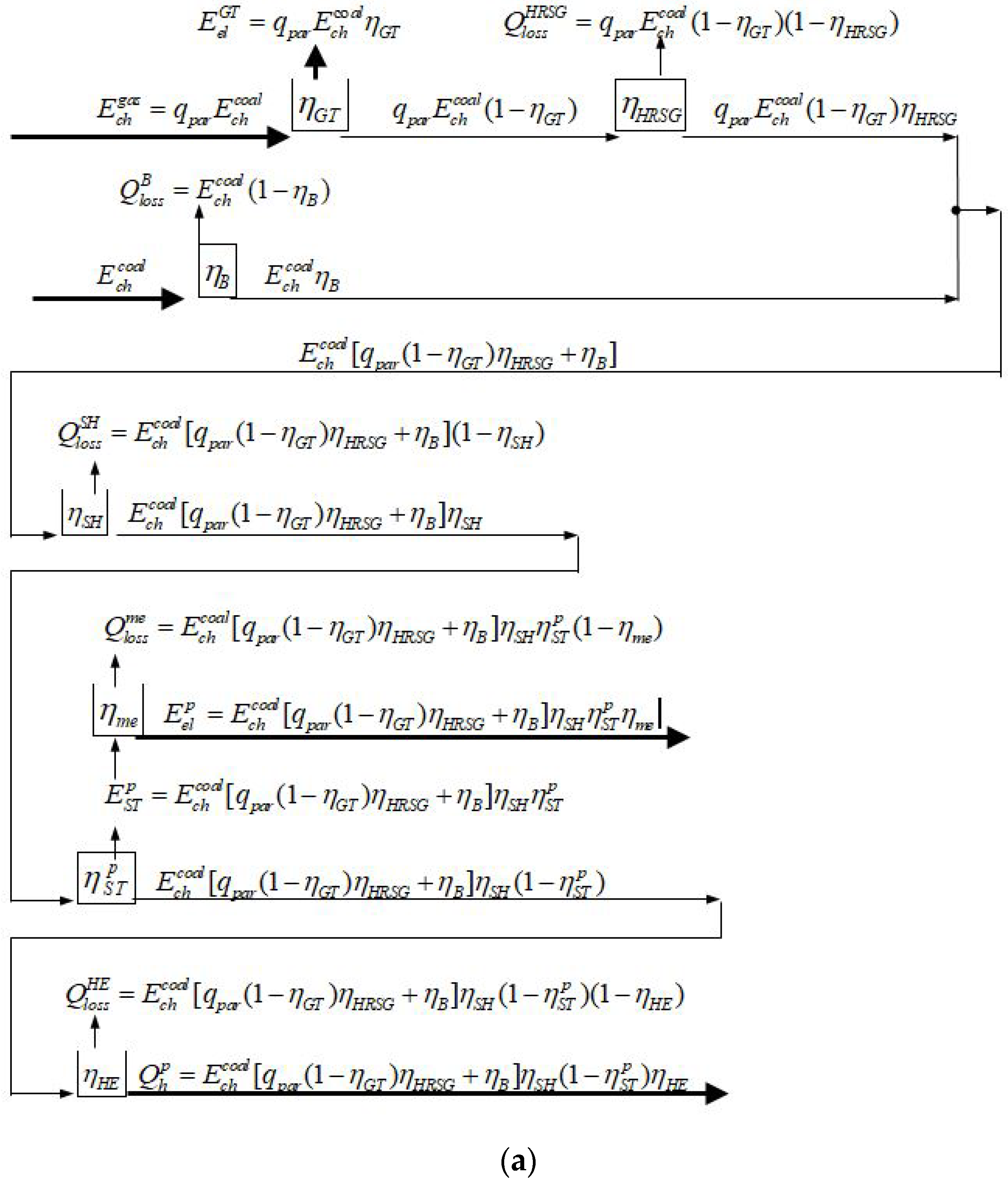
Rectangles in these balances with gross energy efficiencies corresponding to them represent individual devices in the combined heat and power plant to which energy is delivered and extracted. For example, for gas turbine with efficiency ${\eta }_{GT}$, the chemical energy of the gas $E_{ch}^{gas}$ is supplied, and the electricity $E_{el}^{GT}$ and enthalpy of the exhaust gas $q_{par}{E}_{ch}^{coal}(1-{\eta }_{GT})$ are extracted out of it. This enthalpy is then routed to the recovery boiler with the efficiency of ${\eta }_{HRSG}$, etc.

3.1.1. Mathematical Models for the System of Extraction-Backpressure Turbine

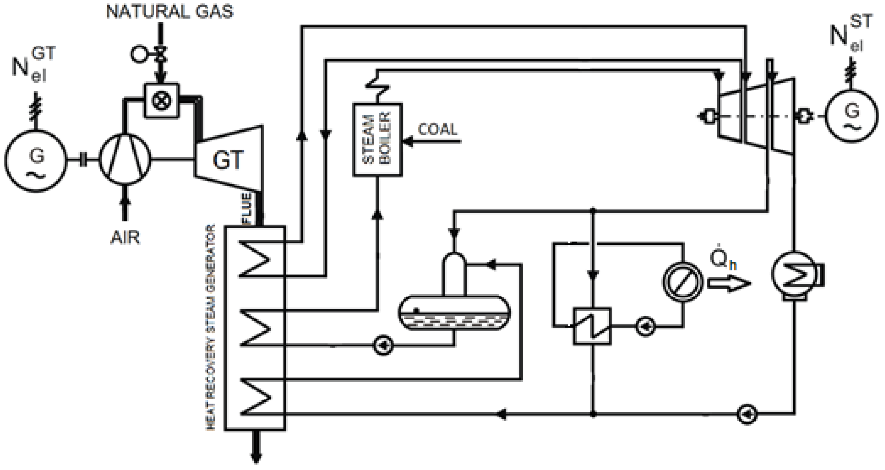
In a dual-fuel gas-steam combined heat and power plant in a parallel system with extraction backpressure steam turbine (Figure 2a), the desired form of the specific average heat production cost, i.e., as a function of the searching value $q_{par}$, is given by:

$$\begin{array}{cc}\hfill k_{h,av}& =\frac{r}{1-{\mathrm{e}}^{-rT}}\{\frac{q_{par}}{[q_{par}(1-{\eta }_{GT}){\eta }_{HRSG}+{\eta }_B]{\eta }_{SH}(1-{\eta }_{ST}^p){\eta }_{HE}}\{(1+x_{sw,m,was})e_{gas}^{t=0}\frac{1}{a_{gas}-r}{[\mathrm{e}}^{(a_{gas}-r)T}-1]+\hfill \\ & +{\rho }_{C{O}_2}^{gas}{p}_{C{O}_2}^{t=0}\frac{1}{a_{C{O}_2}-r}[{\mathrm{e}}^{(a_{C{O}_2}-r)T}-1]+{\rho }_{CO}^{gas}{p}_{CO}^{t=0}\frac{1}{a_{CO}-r}[{\mathrm{e}}^{(a_{CO}-r)T}-1]+\hfill \\ & +{\rho }_{N{O}_X}^{gas}{p}_{N{O}_X}^{t=0}\frac{1}{a_{N{O}_X}-r}[{\mathrm{e}}^{(a_{N{O}_X}-r)T}-1]+{\rho }_{S{O}_2}^{gas}{p}_{S{O}_2}^{t=0}\frac{1}{a_{S{O}_2}-r}[{\mathrm{e}}^{(a_{S{O}_2}-r)T}-1]+\hfill \\ & +{\rho }_{dust}^{gas}{p}_{dust}^{t=0}\frac{1}{a_{dust}-r}{[\mathrm{e}}^{(a_{dust}-r)T}-1]+(1-u){\rho }_{C{O}_2}^{gas}{e}_{C{O}_2}^{t=0}\frac{1}{b_{C{O}_2}-r}{[\mathrm{e}}^{(b_{C{O}_2}-r)T}-1]\}+\hfill \\ & +\frac{1}{[q_{par}(1-{\eta }_{GT}){\eta }_{HRSG}+{\eta }_B]{\eta }_{SH}(1-{\eta }_{ST}^p){\eta }_{HE}}\{(1+x_{sw,m,was})e_{coal}^{t=0}\frac{1}{a_{coal}-r}{[\mathrm{e}}^{(a_{coal}-r)T}-1]+\hfill \\ & +{\rho }_{C{O}_2}^{coal}{p}_{C{O}_2}^{t=0}\frac{1}{a_{C{O}_2}-r}[{\mathrm{e}}^{(a_{C{O}_2}-r)T}-1]+{\rho }_{CO}^{coal}{p}_{CO}^{t=0}\frac{1}{a_{CO}-r}[{\mathrm{e}}^{(a_{CO}-r)T}-1]+\hfill \\ & +{\rho }_{N{O}_X}^{coal}{p}_{N{O}_X}^{t=0}\frac{1}{a_{N{O}_X}-r}[{\mathrm{e}}^{(a_{N{O}_X}-r)T}-1]+{\rho }_{S{O}_2}^{coal}{p}_{S{O}_2}^{t=0}\frac{1}{a_{S{O}_2}-r}[{\mathrm{e}}^{(a_{S{O}_2}-r)T}-1]+\hfill \\ & +{\rho }_{dust}^{coal}{p}_{dust}^{t=0}\frac{1}{a_{dust}-r}[{\mathrm{e}}^{(a_{dust}-r)T}-1]+(1-u){\rho }_{C{O}_2}^{coal}{e}_{C{O}_2}^{t=0}\frac{1}{b_{C{O}_2}-r}{[\mathrm{e}}^{(b_{C{O}_2}-r)T}-1]\}+\hfill \\ & +\frac{i}{{\tau }_s}(1-{\mathrm{e}}^{-rT})(1+x_{sal,t,ins})\frac{{\delta }_{serv}}{r}+\frac{zi}{{\tau }_s}\left(\frac{1-{\mathrm{e}}^{-rT}}{T}+1\right)+\hfill \\ & -\frac{[q_{par}(1-{\eta }_{GT}){\eta }_{HRSG}+{\eta }_B]{\eta }_{SH}{\eta }_{ST}^p{\eta }_{me}+q_{par}{\eta }_{GT}}{[q_{par}(1-{\eta }_{GT}){\eta }_{HRSG}+{\eta }_B]{\eta }_{SH}(1-{\eta }_{ST}^p){\eta }_{HE}}(1-{\epsilon }_{el})e_{el}^{t=0}\frac{1}{a_{el}-r}{[\mathrm{e}}^{(a_{el}-r)T}-1]\}\hfill \end{array}$$

(22)

where:

• i—specific (per unit of power) investment outlay per CHP plant, $i=J/{\dot{Q}}_{h\max }^{CHP}$, (its value depends on the associated technology used for generation of heat and electricity);
• ${\tau }_s$—annual time of using thermal maximum power (peak) heat and power plant ${\dot{Q}}_{h\max }^{CHP}$; $Q_A={\dot{Q}}_{h\max }^{CHP}{\tau }_s$.

This formula was obtained from Formula (19) after substituting the dependencies resulting from the energy balance presented in Figure 2a:

$$\frac{E_{ch,A}^{gas}}{Q_A}=\frac{q_{par}}{[q_{par}(1-{\eta }_{GT}){\eta }_{HRSG}+{\eta }_B]{\eta }_{SH}(1-{\eta }_{ST}^p){\eta }_{HE}},$$

(23)

$$\frac{E_{ch,A}^{coal}}{Q_A}=\frac{1}{[q_{par}(1-{\eta }_{GT}){\eta }_{HRSG}+{\eta }_B]{\eta }_{SH}(1-{\eta }_{ST}^p){\eta }_{HE}},$$

(24)

$$\frac{E_{el,A}^{ST}+E_{el,A}^{GT}}{Q_A}=\frac{[q_{par}(1-{\eta }_{GT}){\eta }_{HRSG}+{\eta }_B]{\eta }_{SH}{\eta }_{ST}^p{\eta }_{me}+q_{par}{\eta }_{GT}}{[q_{par}(1-{\eta }_{GT}){\eta }_{HRSG}+{\eta }_B]{\eta }_{SH}(1-{\eta }_{ST}^p){\eta }_{HE}}.$$

(25)

When calculating from Formula (22) the derivative $d{k}_{h,av}/d{q}_{par}$ is obtained:

$$\begin{array}{l}\frac{d{k}_{h,av}}{d{q}_{par}}=\frac{r}{1-{\mathrm{e}}^{-rT}}\{\frac{{\eta }_B{\eta }_{SH}(1-{\eta }_{ST}^p){\eta }_{HE}}{{\left\{[q_{par}(1-{\eta }_{GT}){\eta }_{HRSG}+{\eta }_B]{\eta }_{SH}(1-{\eta }_{ST}^p){\eta }_{HE}\right\}}^2}\times \\ \hspace{1em}\times \{(1+x_{sw,m,was})e_{gas}^{t=0}\frac{1}{a_{gas}-r}{[\mathrm{e}}^{(a_{gas}-r)T}-1]+\\ \hspace{1em}+{\rho }_{C{O}_2}^{gas}{p}_{C{O}_2}^{t=0}\frac{1}{a_{C{O}_2}-r}[{\mathrm{e}}^{(a_{C{O}_2}-r)T}-1]+{\rho }_{CO}^{gas}{p}_{CO}^{t=0}\frac{1}{a_{CO}-r}[{\mathrm{e}}^{(a_{C{O}_{}}-r)T}-1]+\\ \hspace{1em}+{\rho }_{N{O}_X}^{gas}{p}_{N{O}_X}^{t=0}\frac{1}{a_{N{O}_X}-r}[{\mathrm{e}}^{(a_{N{O}_X}-r)T}-1]+{\rho }_{S{O}_2}^{gas}{p}_{S{O}_2}^{t=0}\frac{1}{a_{S{O}_2}-r}[{\mathrm{e}}^{(a_{S{O}_2}-r)T}-1]+\\ \hspace{1em}+{\rho }_{dust}^{gas}{p}_{dust}^{t=0}\frac{1}{a_{dust}-r}{[\mathrm{e}}^{(a_{dust}-r)T}-1]+(1-u){\rho }_{C{O}_2}^{gas}{e}_{C{O}_2}^{t=0}\frac{1}{b_{C{O}_2}-r}{[\mathrm{e}}^{(b_{C{O}_2}-r)T}-1]\}+\\ \hspace{1em}-\frac{(1-{\eta }_{GT}){\eta }_{HRSG}{\eta }_{SH}^{}(1-{\eta }_{ST}^p){\eta }_{HE}}{{\left\{[q_{par}(1-{\eta }_{GT}){\eta }_{HRSG}+{\eta }_B]{\eta }_{SH}(1-{\eta }_{ST}^p){\eta }_{HE}\right\}}^2}\times \\ \hspace{1em}\times \{(1+x_{sw,m,was})e_{coal}^{t=0}\frac{1}{a_{coal}-r}{[\mathrm{e}}^{(a_{coal}-r)T}-1]+\\ \hspace{1em}+{\rho }_{C{O}_2}^{coal}{p}_{C{O}_2}^{t=0}\frac{1}{a_{C{O}_2}-r}[{\mathrm{e}}^{(a_{C{O}_2}-r)T}-1]+{\rho }_{CO}^{coal}{p}_{CO}^{t=0}\frac{1}{a_{CO}-r}[{\mathrm{e}}^{(a_{CO}-r)T}-1]+\\ \hspace{1em}+{\rho }_{N{O}_X}^{coal}{p}_{N{O}_X}^{t=0}\frac{1}{a_{N{O}_X}-r}[{\mathrm{e}}^{(a_{N{O}_X}-r)T}-1]+{\rho }_{S{O}_2}^{coal}{p}_{S{O}_2}^{t=0}\frac{1}{a_{S{O}_2}-r}[{\mathrm{e}}^{(a_{S{O}_2}-r)T}-1]+\\ \hspace{1em}+{\rho }_{dust}^{coal}{p}_{dust}^{t=0}\frac{1}{a_{dust}-r}[{\mathrm{e}}^{(a_{dust}-r)T}-1]+(1-u){\rho }_{C{O}_2}^{coal}{e}_{C{O}_2}^{t=0}\frac{1}{b_{C{O}_2}-r}{[\mathrm{e}}^{(b_{C{O}_2}-r)T}-1]\}+\\ \hspace{1em}+\{\frac{(1-{\eta }_{GT}){\eta }_{HRSG}{\eta }_{SH}(1-{\eta }_{ST}^p){\eta }_{HE}\left\{[q_{par}(1-{\eta }_{GT}){\eta }_{HRSG}+{\eta }_B]{\eta }_{SH}{\eta }_{ST}^p{\eta }_{me}+q_{par}{\eta }_{GT}\right\}}{{\left\{[q_{par}(1-{\eta }_{GT}){\eta }_{HRSG}+{\eta }_B]{\eta }_{SH}(1-{\eta }_{ST}^p){\eta }_{HE}\right\}}^2}+\\ \hspace{1em}-\frac{[(1-{\eta }_{GT}){\eta }_{HRSG}{\eta }_{SH}{\eta }_{ST}^p{\eta }_{me}+{\eta }_{GT}][q_{par}(1-{\eta }_{GT}){\eta }_{HRSG}+{\eta }_B]{\eta }_{SH}(1-{\eta }_{ST}^p){\eta }_{HE}}{{\left\{[q_{par}(1-{\eta }_{GT}){\eta }_{HRSG}+{\eta }_B]{\eta }_{SH}(1-{\eta }_{ST}^p){\eta }_{HE}\right\}}^2}\}\times \\ \hspace{1em}\times (1-{\epsilon }_{el})e_{el}^{t=0}\frac{1}{a_{el}-r}{[\mathrm{e}}^{(a_{el}-r)T}-1]\}\end{array}$$

(26)

and then from the necessary condition for the existence of an extreme $d{k}_{h,av}/d{q}_{par}=0$, the value of the extremist $q_{par}^{ext}$ cost $k_{h,av}$ is determined:

$$\begin{array}{cc}\hfill 0=& {\eta }_B\{(1+x_{sw,m,was})e_{gas}^{t=0}\frac{1}{a_{gas}-r}{[\mathrm{e}}^{(a_{gas}-r)T}-1]+\hfill \\ & +{\rho }_{C{O}_2}^{gas}{p}_{C{O}_2}^{t=0}\frac{1}{a_{C{O}_2}-r}[{\mathrm{e}}^{(a_{C{O}_2}-r)T}-1]+{\rho }_{CO}^{gas}{p}_{CO}^{t=0}\frac{1}{a_{CO}-r}[{\mathrm{e}}^{(a_{CO}-r)T}-1]+\hfill \\ & +{\rho }_{N{O}_X}^{gas}{p}_{N{O}_X}^{t=0}\frac{1}{a_{N{O}_X}-r}[{\mathrm{e}}^{(a_{N{O}_X}-r)T}-1]+{\rho }_{S{O}_2}^{gas}{p}_{S{O}_2}^{t=0}\frac{1}{a_{S{O}_2}-r}[{\mathrm{e}}^{(a_{S{O}_2}-r)T}-1]+\hfill \\ & +{\rho }_{dust}^{gas}{p}_{dust}^{t=0}\frac{1}{a_{dust}-r}{[\mathrm{e}}^{(a_{dust}-r)T}-1]+(1-u){\rho }_{C{O}_2}^{gas}{e}_{C{O}_2}^{t=0}\frac{1}{b_{C{O}_2}-r}{[\mathrm{e}}^{(b_{C{O}_2}-r)T}-1]\}+\hfill \\ & -(1-{\eta }_{GT}){\eta }_{HRSG}\{(1+x_{sw,m,was})e_{coal}^{t=0}\frac{1}{a_{coal}-r}{[\mathrm{e}}^{(a_{coal}-r)T}-1]+\hfill \\ & +{\rho }_{C{O}_2}^{coal}{p}_{C{O}_2}^{t=0}\frac{1}{a_{C{O}_2}-r}[{\mathrm{e}}^{(a_{C{O}_2}-r)T}-1]+{\rho }_{CO}^{coal}{p}_{CO}^{t=0}\frac{1}{a_{CO}-r}[{\mathrm{e}}^{(a_{CO}-r)T}-1]+\hfill \\ & +{\rho }_{N{O}_X}^{coal}{p}_{N{O}_X}^{t=0}\frac{1}{a_{N{O}_X}-r}[{\mathrm{e}}^{(a_{N{O}_X}-r)T}-1]+{\rho }_{S{O}_2}^{coal}{p}_{S{O}_2}^{t=0}\frac{1}{a_{S{O}_2}-r}[{\mathrm{e}}^{(a_{S{O}_2}-r)T}-1]+\hfill \\ & +{\rho }_{dust}^{coal}{p}_{dust}^{t=0}\frac{1}{a_{dust}-r}[{\mathrm{e}}^{(a_{dust}-r)T}-1]+(1-u){\rho }_{C{O}_2}^{coal}{e}_{C{O}_2}^{t=0}\frac{1}{b_{C{O}_2}-r}{[\mathrm{e}}^{(b_{C{O}_2}-r)T}-1]\}+\hfill \\ & -{\eta }_{GT}{\eta }_B(1-{\epsilon }_{el})e_{el}^{t=0}\frac{1}{a_{el}-r}[{\mathrm{e}}^{(a_{el}-r)T}-1].\hfill \end{array}$$

(27)

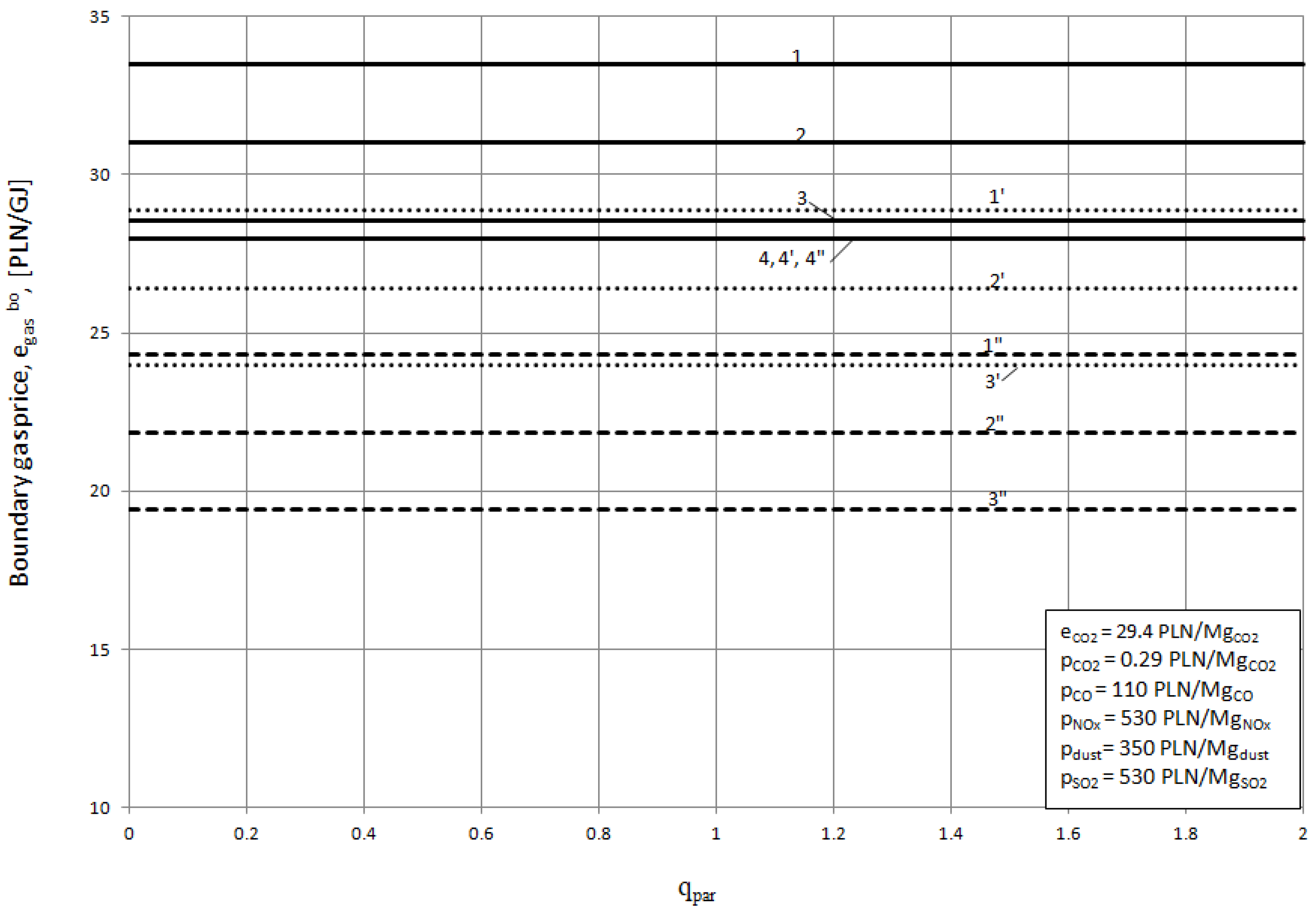
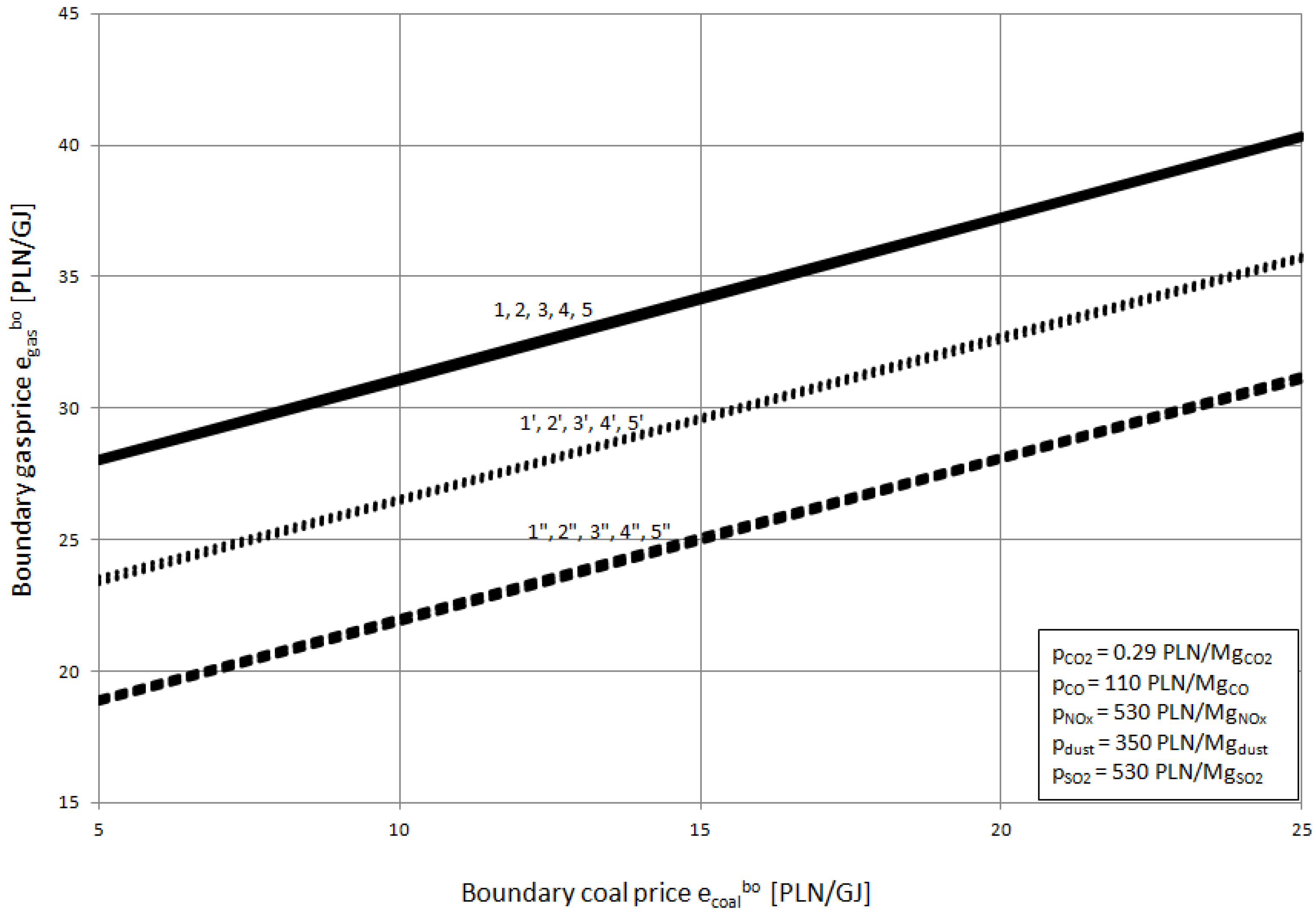
As we can see from Formula (27), the value $q_{par}^{ext}$ which forms the extreme of the cost $k_{h,av}$ does not exist. This is because this value in the Formula (27) does not occur (this situation can be changed by development of a relation which relates the specific investment “i” to the value of $q_{par}$) From Formula (27), however, it is possible to determine the boundary prices of gas $e_{gas}^{bo}$ and coal $e_{coal}^{bo}$ for a given electricity price, i.e., for the prices where the cost $k_{h,av}$ assumes a constant value, and therefore is independent of $q_{par}$, since then the derivative fulfills the condition $d{k}_{h,av}/d{q}_{par}=0$.

Thus, for a given price of coal $e_{coal}$ and electricity $e_{el}$ derived from Formula (27), a boundary price of the gas $e_{gas}^{bo}$ can be set, and vice versa, the boundary price of coal $e_{coal}^{bo}$ is determined for a given prices of gas $e_{gas}$ and electricity $e_{el}$. Thus, the boundary prices of gas and coal are closely related (Figures 6 and 7) and substituted into the formula in (26), which leads to the value of zero obtained in this formula. On the other hand, if other values are inserted into Formula (26), for example current coal and gas prices (current coal and gas prices in Poland are equal to $e_{coal}=11.4\mathrm{PLN}/\mathrm{GJ}$, $e_{gas}=28\mathrm{PLN}/\mathrm{GJ}$), which is different from boundary values, and the formula takes a positive or negative value.

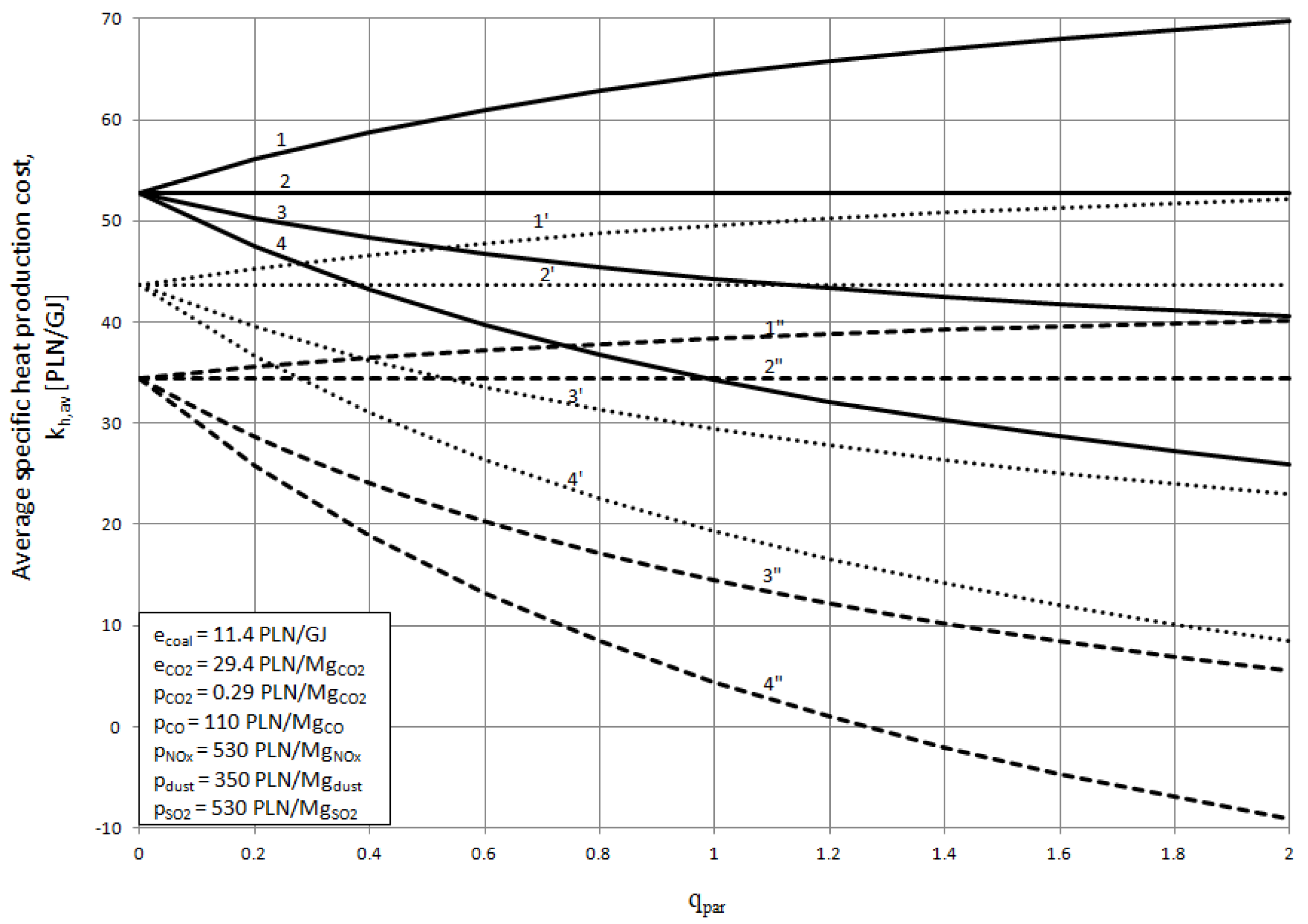
If the cost of gas in Formula (27) exceeds the costs associated with coal combustion, then $d{k}_{h,av}/d{q}_{par}>0$ and the cost $k_{h,av}$ increases along with a higher value of $q_{par}$, and vice versa, when the cost associated with gas is lower than the cost associated with coal, and then the relation $d{k}_{h,av}/d{q}_{par}<0$ is met and the cost $k_{h,av}$ decreases along with the increase in the capacity of the gas turbine set. However, it should be noted that the relation $d{k}_{h,av}/d{q}_{par}<0$ is possible in two cases. Firstly, when the price of coal is higher than its boundary price (then the cost of heat production $k_{h,av}$ is the highest, Figures 4 and 9) and secondly, when the price of gas is lower than its boundary price (then the cost $k_{h,av}$ is the lowest, Figures 3 and 8).

Therefore, the necessary condition for the economic feasibility of an investment in a dual-fuel gas-steam CHP plant compared to a coal-fired CHP plant (i.e., $q_{par}=0$, Figures 3 and 8), needs to involve not only an assumption that the relation $d{k}_{h,av}/d{q}_{par}<0$ is met, but also the gas price has to be lower than its boundary price determined from Formula (27) for the current coal and electricity prices.

The necessary condition for the profitability of the construction of dual-fuel CHP plants should, therefore, be finally expressed by means of the following relation:

$$e_{gas}\le e_{gas}^{bo}.$$

(28)

The higher the prices of electricity $e_{el}$ and coal $e_{coal}$, the higher the boundary value $e_{gas}^{bo}$, and thus the price of gas, for which the construction of dual-fuel gas-steam CHP plant will be feasible can be higher (Figures 6 and 7).

If the relationship $e_{gas}\le e_{gas}^{bo}$ is fulfilled, the gas turbine set with the maximum capacity forms the most profitable alternative, and the greatest value $q_{par}=q_{par}^{\max }$ is then obtained (Formula (21)). Therefore, knowledge of the boundary price of coal $e_{coal}^{bo}$ and gas $e_{gas}^{bo}$ offers very important inputs for the analysis.

With the input of these values, we are able to answer the question whether a dual-fuel gas-steam combined heat and power plant is more economically feasible for the current gas and electricity and coal prices, as well as emission charges on harmful products emitted into the environment in connection with the power unit’s operation and the investment made in its construction, or whether it is more profitable to build a single coal-fired CHP plant.

We should also note that the higher the ratio of the price of electricity $e_{el}$ to the prices of fuels $e_{coal}$, $e_{gas}$ (especially expensive gas $e_{gas}$), the lower the specific cost of heat production $k_{h,av}$ (Formula (19)).

The revenue from the sale of electricity produced in the combined heat and power plant increases with the increase of $e_{el}$, which takes on a minus sign as the avoided cost of heat production: $-\left(E_{el,A}^{ST}+E_{el,A}^{GT}\right)(1-{\epsilon }_{el})e_{el}^{t=0}\frac{1}{a_{el}-r}{[\mathrm{e}}^{(a_{el}-r)T}-1]$ (Formula (19)).

This revenue also increases along with higher electricity output, so the higher capacity of the gas turbine leads to higher value of $q_{par}$. If this income is higher from the cost of heat production, then the specific cost $k_{h,av}$ takes on a negative value—Figure 8. Curve 4”—and therefore NPV profit (Formula (13)) that is obtained from the operation of combined heat and power plant is greater.

3.1.2. Mathematical Models of a System with Extraction-Condensing Turbine

In a dual-fuel gas-steam combined heat and power plant with an extraction-condensing steam turbine operating in a parallel system (Figure 2b), the form of the average specific cost of heat production, i.e., as a function of the value $q_{par}$, is given by:

$$\begin{array}{cc}\hfill k_{h,av}& =\frac{r}{1-{\mathrm{e}}^{-rT}}\{\frac{q_{par}}{\beta [q_{par}(1-{\eta }_{GT}){\eta }_{HRSG}+{\eta }_B]{\eta }_{SH}{\eta }_{ST}^k{\eta }_{HE}}\{(1+x_{sw,m,was})e_{gas}^{t=0}\frac{1}{a_{gas}-r}{[\mathrm{e}}^{(a_{gas}-r)T}-1]+\hfill \\ & +{\rho }_{C{O}_2}^{gas}{p}_{C{O}_2}^{t=0}\frac{1}{a_{C{O}_2}-r}[{\mathrm{e}}^{(a_{C{O}_2}-r)T}-1]+{\rho }_{CO}^{gas}{p}_{CO}^{t=0}\frac{1}{a_{CO}-r}[{\mathrm{e}}^{(a_{CO}-r)T}-1]+\hfill \\ & +{\rho }_{N{O}_X}^{gas}{p}_{N{O}_X}^{t=0}\frac{1}{a_{N{O}_X}-r}[{\mathrm{e}}^{(a_{N{O}_X}-r)T}-1]+{\rho }_{S{O}_2}^{gas}{p}_{S{O}_2}^{t=0}\frac{1}{a_{S{O}_2}-r}[{\mathrm{e}}^{(a_{S{O}_2}-r)T}-1]+\hfill \\ & +{\rho }_{dust}^{gas}{p}_{dust}^{t=0}\frac{1}{a_{dust}-r}{[\mathrm{e}}^{(a_{dust}-r)T}-1]+(1-u){\rho }_{C{O}_2}^{gas}{e}_{C{O}_2}^{t=0}\frac{1}{b_{C{O}_2}-r}{[\mathrm{e}}^{(b_{C{O}_2}-r)T}-1]\}+\hfill \\ & +\frac{1}{\beta [q_{par}(1-{\eta }_{GT}){\eta }_{HRSG}+{\eta }_B]{\eta }_{SH}{\eta }_{ST}^k{\eta }_{HE}}\{(1+x_{sw,m,was})e_{coal}^{t=0}\frac{1}{a_{coal}-r}{[\mathrm{e}}^{(a_{coal}-r)T}-1]+\hfill \\ & +{\rho }_{C{O}_2}^{coal}{p}_{C{O}_2}^{t=0}\frac{1}{a_{C{O}_2}-r}[{\mathrm{e}}^{(a_{C{O}_2}-r)T}-1]+{\rho }_{CO}^{coal}{p}_{CO}^{t=0}\frac{1}{a_{CO}-r}[{\mathrm{e}}^{(a_{CO}-r)T}-1]+\hfill \\ & +{\rho }_{N{O}_X}^{coal}{p}_{N{O}_X}^{t=0}\frac{1}{a_{N{O}_X}-r}[{\mathrm{e}}^{(a_{N{O}_X}-r)T}-1]+{\rho }_{S{O}_2}^{coal}{p}_{S{O}_2}^{t=0}\frac{1}{a_{S{O}_2}-r}[{\mathrm{e}}^{(a_{S{O}_2}-r)T}-1]+\hfill \\ & +{\rho }_{dust}^{coal}{p}_{dust}^{t=0}\frac{1}{a_{dust}-r}[{\mathrm{e}}^{(a_{dust}-r)T}-1]+(1-u){\rho }_{C{O}_2}^{coal}{e}_{C{O}_2}^{t=0}\frac{1}{b_{C{O}_2}-r}{[\mathrm{e}}^{(b_{C{O}_2}-r)T}-1]\}+\hfill \\ & +\frac{i}{{\tau }_s}(1-{\mathrm{e}}^{-rT})(1+x_{sal,t,ins})\frac{{\delta }_{serv}}{r}+\frac{zi}{{\tau }_s}\left(\frac{1-{\mathrm{e}}^{-rT}}{T}+1\right)+\hfill \\ & -\frac{[q_{par}(1-{\eta }_{GT}){\eta }_{HRSG}+{\eta }_B]{\eta }_{SH}{\eta }_{ST}^k{\eta }_{me}+q_{par}{\eta }_{GT}}{\beta [q_{par}(1-{\eta }_{GT}){\eta }_{HRSG}+{\eta }_B]{\eta }_{SH}{\eta }_{ST}^k{\eta }_{HE}}(1-{\epsilon }_{el})e_{el}^{t=0}\frac{1}{a_{el}-r}{[\mathrm{e}}^{(a_{el}-r)T}-1]\}.\hfill \end{array}$$

(29)

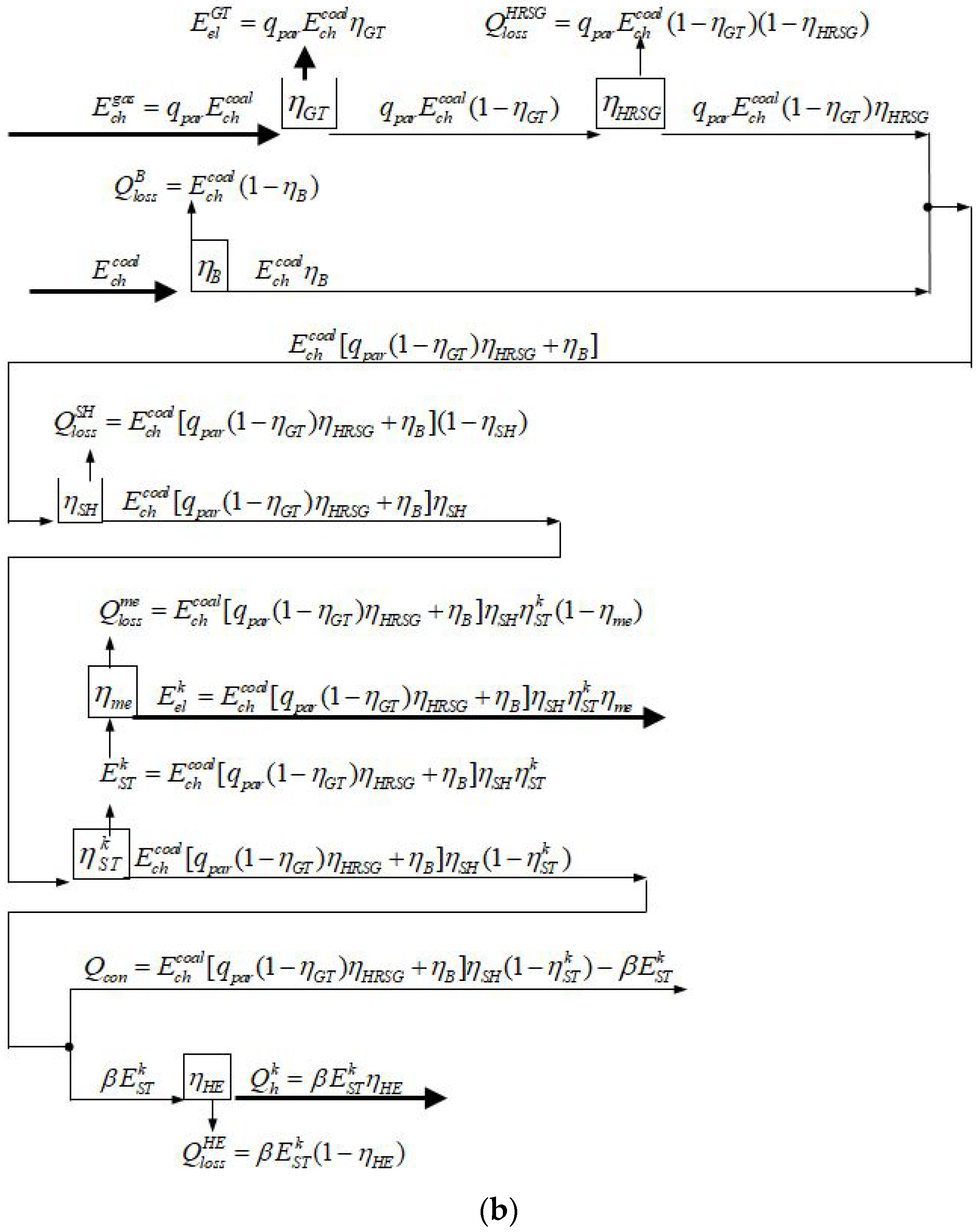
This formula was obtained from Formula (19) after substituting the dependencies resulting from the energy balance presented in Figure 2b:

$$\frac{E_{ch,A}^{gas}}{Q_A}=\frac{q_{par}}{\beta [q_{par}(1-{\eta }_{GT}){\eta }_{HRSG}+{\eta }_B]{\eta }_{SH}{\eta }_{ST}^k{\eta }_{HE}},$$

(30)

$$\frac{E_{ch,A}^{coal}}{Q_A}=\frac{1}{\beta [q_{par}(1-{\eta }_{GT}){\eta }_{HRSG}+{\eta }_B]{\eta }_{SH}{\eta }_{ST}^k{\eta }_{HE}},$$

(31)

$$\frac{E_{el,A}^{ST}+E_{el,A}^{GT}}{Q_A}=\frac{[q_{par}(1-{\eta }_{GT}){\eta }_{HRSG}+{\eta }_B]{\eta }_{SH}{\eta }_{ST}^k{\eta }_{me}+q_{par}{\eta }_{GT}}{\beta [q_{par}(1-{\eta }_{GT}){\eta }_{HRSG}+{\eta }_B]{\eta }_{SH}{\eta }_{ST}^k{\eta }_{HE}}.$$

(32)

When we calculate the derivative of $d{k}_{h,av}/d{q}_{par}$ from the formula in (29), the following relation is obtained:

$$\begin{array}{l}\frac{d{k}_{h,av}}{d{q}_{par}}=\frac{r}{1-{\mathrm{e}}^{-rT}}\{\frac{\beta {\eta }_B{\eta }_{SH}{\eta }_{ST}^k{\eta }_{HE}}{{\left\{\beta [q_{par}(1-{\eta }_{GT}){\eta }_{HRSG}+{\eta }_B]{\eta }_{SH}{\eta }_{ST}^k{\eta }_{HE}\right\}}^2}\times \\ \hspace{1em}\times \{(1+x_{sw,m,was})e_{gas}^{t=0}\frac{1}{a_{gas}-r}{[\mathrm{e}}^{(a_{gas}-r)T}-1]+\\ \hspace{1em}+{\rho }_{C{O}_2}^{gas}{p}_{C{O}_2}^{t=0}\frac{1}{a_{C{O}_2}-r}[{\mathrm{e}}^{(a_{C{O}_2}-r)T}-1]+{\rho }_{CO}^{gas}{p}_{CO}^{t=0}\frac{1}{a_{CO}-r}[{\mathrm{e}}^{(a_{CO}-r)T}-1]+\\ \hspace{1em}+{\rho }_{N{O}_X}^{gas}{p}_{N{O}_X}^{t=0}\frac{1}{a_{N{O}_X}-r}[{\mathrm{e}}^{(a_{N{O}_X}-r)T}-1]+{\rho }_{S{O}_2}^{gas}{p}_{S{O}_2}^{t=0}\frac{1}{a_{S{O}_2}-r}[{\mathrm{e}}^{(a_{S{O}_2}-r)T}-1]+\\ \hspace{1em}+{\rho }_{dust}^{gas}{p}_{dust}^{t=0}\frac{1}{a_{dust}-r}{[\mathrm{e}}^{(a_{dust}-r)T}-1]+(1-u){\rho }_{C{O}_2}^{gas}{e}_{C{O}_2}^{t=0}\frac{1}{b_{C{O}_2}-r}{[\mathrm{e}}^{(b_{C{O}_2}-r)T}-1]\}+\\ \hspace{1em}-\frac{\beta (1-{\eta }_{GT}){\eta }_{HRSG}{\eta }_{SH}{\eta }_{ST}^k{\eta }_{HE}}{{\left\{\beta [q_{par}(1-{\eta }_{GT}){\eta }_{HRSG}+{\eta }_B]{\eta }_{SH}{\eta }_{ST}^k{\eta }_{HE}\right\}}^2}\times \\ \hspace{1em}\times \{(1+x_{sw,m,was})e_{coal}^{t=0}\frac{1}{a_{coal}-r}{[\mathrm{e}}^{(a_{coal}-r)T}-1]+\\ \hspace{1em}+{\rho }_{C{O}_2}^{coal}{p}_{C{O}_2}^{t=0}\frac{1}{a_{C{O}_2}-r}[{\mathrm{e}}^{(a_{C{O}_2}-r)T}-1]+{\rho }_{CO}^{coal}{p}_{CO}^{t=0}\frac{1}{a_{CO}-r}[{\mathrm{e}}^{(a_{CO}-r)T}-1]+\\ \hspace{1em}+{\rho }_{N{O}_X}^{coal}{p}_{N{O}_X}^{t=0}\frac{1}{a_{N{O}_X}-r}[{\mathrm{e}}^{(a_{N{O}_X}-r)T}-1]+{\rho }_{S{O}_2}^{coal}{p}_{S{O}_2}^{t=0}\frac{1}{a_{S{O}_2}-r}[{\mathrm{e}}^{(a_{S{O}_2}-r)T}-1]+\\ \hspace{1em}+{\rho }_{dust}^{coal}{p}_{dust}^{t=0}\frac{1}{a_{dust}-r}[{\mathrm{e}}^{(a_{dust}-r)T}-1]+(1-u){\rho }_{C{O}_2}^{coal}{e}_{C{O}_2}^{t=0}\frac{1}{b_{C{O}_2}-r}{[\mathrm{e}}^{(b_{C{O}_2}-r)T}-1]\}+\\ \hspace{1em}+\{\frac{\beta (1-{\eta }_{GT}){\eta }_{HRSG}{\eta }_{SH}{\eta }_{ST}^k{\eta }_{HE}\left\{[q_{par}(1-{\eta }_{GT}){\eta }_{HRSG}+{\eta }_B]{\eta }_{SH}{\eta }_{ST}^k{\eta }_{me}^{}+q_{par}{\eta }_{GT}\right\}}{{\left\{\beta [q_{par}(1-{\eta }_{GT}){\eta }_{HRSG}+{\eta }_B]{\eta }_{SH}{\eta }_{ST}^k{\eta }_{HE}\right\}}^2}+\\ \hspace{1em}-\frac{[(1-{\eta }_{GT}){\eta }_{HRSG}{\eta }_{SH}{\eta }_{ST}^k{\eta }_{me}+{\eta }_{GT}][q_{par}(1-{\eta }_{GT}){\eta }_{HRSG}+{\eta }_B]\beta {\eta }_{SH}{\eta }_{ST}^k{\eta }_{HE}}{{\left\{\beta [q_{par}(1-{\eta }_{GT}){\eta }_{HRSG}+{\eta }_B]{\eta }_{SH}{\eta }_{ST}^k{\eta }_{HE}\right\}}^2}\}\times \\ \hspace{1em}\times (1-{\epsilon }_{el})e_{el}^{t=0}\frac{1}{a_{el}-r}{[\mathrm{e}}^{(a_{el}-r)T}-1]\}\end{array}$$

(33)

and from this dependence for the necessary condition regarding the existence of the extreme $k_{h,av}$ of the cost, i.e., resulting in zeroing the derivative $d{k}_{h,av}/d{q}_{par}=0$, and an identical formula is obtained as that in Formula (27). This comes as a consequence of adoption of a lack of a dependence between the specific investment “i” and the variable $q_{par}$ in the mathematical model. The boundary gas price in the case of its combustion in a combined heat and power plant—Figures 6 and 7—for given coal and electricity prices does not depend on the type of steam turbine installed in it, despite the fact that the specific cost $k_{h,av}$ apparently is relative to it. This is because the specific investment is greater for a combined heat and power plant with an extraction-condensing steam turbine than for an extraction-backpressure steam turbine. This results from the necessity of incurring a cost associated with the steam condenser and the cooling tower in the system comprising an extraction-condensing turbine, whereas this cost does not occur in a system with an extraction-backpressure turbine.

In the calculations, it was assumed that specific investment in a combined heat and power plant with an extraction-condensing steam turbine is equal to i = 4.6 million PLN/MW, whereas for a combined heat and power plant with extraction-backpressure turbine, this cost is equal to i = 4 million PLN/MW. At the same time, in the present study it was assumed that the efficiency of the Clausius–Rankine cycle of the extraction-condensing steam turbine is ${\eta }_{ST}={\eta }_{CR}{\eta }_i$ = 0.45, and the extraction-backpressure turbine it is equal to ${\eta }_{ST}={\eta }_{CR}{\eta }_i$ = 0.4. The following input values were also adopted in the calculations: b = 4 years, β = 2, ${\eta }_{GT}$ = 0.35, ${\eta }_{HRSG}$ = 0.85, ${\eta }_B$ = 0.9, ${\eta }_{SH}$ = 0.98, ${\eta }_{me}$ = 0.98, ${\eta }_{HE}$ = 0.95, ${\epsilon }_{el}$ = 0.04, δ_serv = 0.03, r = 7%, ${\tau }_s$ = 3000 h/a, T = 20 years. All calculation results presented in the paper correspond to zero values of all exponents $a_{el}$, $a_{gas}$, $a_{coal}$, $a_{{CO}_2}$, $a_{CO}$, $a_{{SO}_2}$, $a_{{NO}_X}$, $a_{dust}$, $b_{{CO}_2}$. Thus, the prices of energy carriers and environmental fees are constant over the whole operation period T of a combined heat and power plant, and they form integral mean values over the T period. For example, the integral mean value of the electricity price varying in time according to the formula $e_{el}(t)=e_{el}^{t=0}{\mathrm{e}}^{a_{el}t}$ is calculated according to the formula:

$$e_{el}^{av}=\frac{1}{T}{\displaystyle \underset{0}{\overset{T}{\int }}{e}_{el}^{t=0}{\mathrm{e}}^{a_{el}t}dt}=\frac{e_{el}^{t=0}}{T{a}_{el}}\left({\mathrm{e}}^{a_{el}T}-1\right).$$

(34)

The value of the chemical energy share of fuel in its total annual consumption was also used for calculations, for which CO₂ emission allowances are not required, u = 0, because from 2020 there will no longer be free emission allocations. This means that all installations will have to pay for each tonne of the carbon dioxide that is emitted. Formulas (22) and (29) can also be used to analyze the impact of technical and economic parameters on the specific cost of heat production. This analysis is most conveniently carried out using differential calculus [26]. As demonstrated in [26], this cost is most sensitive to fuel prices and relations between them. However, technical parameters as well as the efficiency of equipment, have a relatively small impact.

4. Results and Discussion

Figures 3–5 and 8–10 show exemplary results of calculations of the average specific heat production cost $k_{h,av}$ (Formula (19)) in a dual-fuel gas-steam combined heat and power plant. They are presented for two alternatives: for a combined heat and power plant with an extraction-condensing turbine, and for the case of an extraction-backpressure turbine. The analysis here also accounts for the economic parameters that have the greatest impact on this cost. Figures 6 and 7 also show the boundary prices of gas $e_{gas}^{bo}$ and coal $e_{coal}^{bo}$ with the electricity prices and the purchase of CO₂ emission allowances as the parameters. For prices $e_{gas}^{bo}$, $e_{coal}^{bo}$, the cost $k_{h,av}$ is constant and independent of the value $q_{par}$. The lines of this cost are, therefore, horizontal in function $q_{par}$ (Figures 3–5 and 8–10). The amount of data in the individual figures is huge. If we remove some of it to reduce the volume of the data in the figures, it would be apparently easier for the reader to analyze the information. However, this would limit the volume of the relevant information regarding the course of the value of $k_{h,av}$ depending on the price of gas, coal, electricity and environmental charges.

4.1. Combined Heat and Power Plant Comprising an Extraction-Condensing Turbine

In Figure 3, the curves 3, 3’, 3”, 4, 4’, 4” are decreasing because the costs of gas in Formula (33) is lower than costs associated with coal and, as a consequence, $d{k}_{h,av}/d{q}_{par}<0$. The values of these curves are calculated for gas prices lower than its limit prices equal to: $e_{gas}^{bo}$ = 22.71 PLN/GJ (for $e_{el}$ = 170 PLN/MWh), $e_{gas}^{bo}$ = 27.29 PLN/GJ (for $e_{el}$ = 220 PLN/MWh), $e_{gas}^{bo}$ = 31.86 PLN/GJ (for $e_{el}$ = 270 PLN/MWh). The gas limit prices correspond to the current price of coal equal to $e_{coal}=11.4\mathrm{PLN}/\mathrm{GJ}$ and current purchase price of CO₂ emission allowances equal to $e_{{CO}_2}$ = 29.4 PLN/Mg. Curves 1, 1’, 1” have an increasing characteristic as the price of gas is higher for them than the boundary prices, and therefore the costs related to gas in Formula (33) exceed the costs associated with coal and $d{k}_{h,av}/d{q}_{par}>0$. As we can see from the course of curves 3, 3’, 3”, 4, 4’, 4”, a dual-fuel gas-steam CHP plant is more economically feasible than a single coal-fired CHP plant if the gas price is lower than its boundary prices of coal and electricity.

The specific heat production cost $k_{h,av}$ is then the smallest for the maximum capacity of the gas turbine set. For the current price of coal $e_{coal}=11.4\mathrm{PLN}/\mathrm{GJ}$ and electricity prices $e_{el}$ = 170 PLN/MWh, the price of gas needs to be below the price $e_{gas}^{bo}$ = 22.71 PLN/GJ. The current gas price in Poland is equal to $e_{gas}=28\mathrm{PLN}/\mathrm{GJ}$ and dual-fuel gas-steam combined heat and power plants are, therefore, unprofitable.

The curves 3, 3’, 3” in Figure 4 have an increasing course since the cost of gas in Formula (33) outweighs the costs associated with coal. The values of these curves are calculated for prices of coal $e_{coal}$ below its boundary prices equal to: $e_{coal}^{bo}$ = 20 PLN/GJ (for $e_{el}$ = 170 PLN/MWh), $e_{coal}^{bo}$ = 12.55 PLN/GJ (for $e_{el}$ = 220 PLN/MWh), $e_{coal}^{bo}$ = 5.11 PLN/GJ (for $e_{el}$ = 270 PLN/MWh) (curves 2, 2’, 2”). The boundary prices of coal applied in the analysis correspond to the current price of gas equal to $e_{gas}=28\mathrm{PLN}/\mathrm{GJ}$ and current price for the purchase of CO₂ emission allowances $e_{{CO}_2}$ = 29.4 PLN/Mg. On the other hand, the curves 1, 1’, 1” have a decreasing course since they were developed for the price of coal higher than the boundary ones, and therefore the relation $d{k}_{h,av}/d{q}_{par}<0$ is fulfilled. The cost of heat production $k_{h,av}$ is also the highest due to the highest price of coal and high gas price.

Figure 5 demonstrates the impact of the purchase price of $e_{{CO}_2}$ allowances for a tonne of carbon dioxide emission on the specific heat production cost $k_{h,av}$. The higher the $e_{{CO}_2}$ price, the higher the $e_{coal}^{bo}$ boundary value, so the higher the price of gas for which the construction of dual-fuel gas-steam CHP plant will be economically feasible. This does not mean, however, that the increase of the price $e_{{CO}_2}$ offers better economic results. Actually, it is the opposite. An increase in the $e_{{CO}_2}$ price results in an increase in the cost $k_{h,av}$.

The curves 4, 5, 6 in Figure 5 take an increasing course for the same reason as the curves in Figure 3 and Figure 4. The values of these curves were calculated for the price of coal $e_{coal}=11.4\mathrm{PLN}/\mathrm{GJ}$ lower than its boundary prices equal to: $e_{coal}^{bo}$ = 19.64 PLN/GJ (for $e_{{CO}_2}$ = 100 PLN/Mg, $e_{el}$ = 170 PLN/MWh), $e_{coal}^{bo}$ = 19.86 PLN/GJ (for $e_{{CO}_2}$ = 60 PLN/Mg, $e_{el}$ = 170 PLN/MWh), $e_{coal}^{bo}$ = 20.08 PLN/GJ (for $e_{{CO}_2}$ = 20 PLN/Mg, $e_{el}$ = 170 PLN/MWh) (curves 1, 2, 3). All boundary prices of coal correspond to the price of gas equal to $e_{gas}=28\mathrm{PLN}/\mathrm{GJ}$.

Figure 6 shows the gas $e_{gas}^{bo}$ and coal $e_{coal}^{bo}$ boundary prices calculated by application of the Formula (27), i.e., for the prices for which the cost $k_{h,av}$ assumes a constant value independent of $q_{par}$. The higher the boundary coal price, the higher the boundary gas price, and vice versa. As can be concluded from the necessary condition stated in (28), the higher the price $e_{gas}^{bo}$, the higher the price $e_{gas}$ for which the construction of a dual-fuel gas-steam CHP plant is profitable.

Figure 7 presents the range of the boundary values of gas price $e_{gas}^{bo}$ as a function of the boundary price of coal $e_{coal}^{bo}$ and electricity price expressed as $e_{el}$ and carbon dioxide emission allowances $e_{{CO}_2}$ as the parameters.

As we can conclude from the course of the curves in Figure 7, the boundary prices of gas and coal in a dual-fuel gas-steam CHP plants depend to the greatest extent to the price of electricity $e_{el}$. The purchase price $e_{{CO}_2}$ of permits for the emission of a tonne of CO₂ affects these prices to a negligible level.

4.2. Combined Heat and Power Plants with a Backpressure Turbine

Figure 8, Figure 9 and Figure 10 show the results of calculations of the specific cost of heat production $k_{h,av}$ for a combined heat and power plant with an extraction-backpressure steam turbine. The characteristics of the individual curves in these figures are identical to the courses of the corresponding curves in Figure 3, Figure 4 and Figure 5 prepared for a combined heat and power plant with an extraction-condensing turbine. The only difference is that they contain lower values of the cost $k_{h,av}$ corresponding to the same energy prices and environmental fees.

This is due to the fact that the total energy efficiency of the backpressure turbine cycle is greater from the efficiency of the condensing turbine, although the range of application of enthalpy of steam for the production of electricity is smaller in it, on condition that the same parameters of fresh steam are considered. As mentioned above, the efficiency of electricity generation in the Clausius–Rankine cycle of the extraction-condensing steam turbine was assumed at the level of ${\eta }_{ST}$ = 0.45, and for the cycle with the extraction-backpressure turbine equal to ${\eta }_{ST}$ = 0.4.

The lower cost $k_{h,av}$, along with the higher total energy efficiency of the system with the extraction-backpressure turbine, also comes as a result of smaller specific investment. In this system, as mentioned above the under-turbine condenser and the cooling tower, are unnecessary, although they are necessary in the system with a condensing turbine.

The boundary prices of coal and gas for a given electricity price for combined heat and power plants with an extraction backpressure steam turbine are also presented in Figure 6 and Figure 7. As already stated above, the gas and coal boundary prices do not depend on the type of steam turbine set installed in the CHP plant.

5. Conclusions

The methodologies and mathematical models presented in the paper were applied for the technical and economic analysis of the operation of the CHP plant in dual-fuel gas technology in a parallel system, and calculations were performed for a number of technical alternatives, as presented in Figure 3, Figure 4, Figure 5, Figure 6, Figure 7, Figure 8, Figure 9 and Figure 10. They are presented for the alternatives comprising a combined heat and power plant with an extraction-condensing steam turbine and an extraction backpressure steam turbine for a wide range of the variability in energy prices and environmental charges and, therefore, also for current prices and environmental fees. All the graphs were obtained by the application of the innovative methodology and by use of a mathematical model in the expression developed for the total, discounted for the current moment NPV profit resulting from the operation of a dual-fuel gas-steam CHP plant (Formula (13)).

The decisive values of the power of the gas turbine set $N_{el\max }^{GT}$ include the prices of gas, coal, electricity, environmental costs and capital expenditures. The fuel prices and outlays are lower, and the higher the price of electricity, the lower the specific cost of heat production $k_{h,av}$ (Formula (19)).

A necessary condition for the cost-effectiveness of the construction of dual-fuel gas-steam CHP plants, and hence their greater profitability from single coal CHP plants, is associated with the fulfillment of the relation $e_{gas}\le e_{gas}^{bo}$ (Formula (28)), i.e., a condition that the gas price needs to be lower than its boundary value. What is more, the lower the price of gas than the boundary price (determined for the current coal and electricity prices), the lower is the specific cost of heat production $k_{h,av}$ and the most advantageous is the maximum power of the gas turbine set $N_{el\max }^{GT}$—curves 3, 3’, 3”, 4, 4’, 4” in Figure 3 and Figure 8.

The higher the purchase price $e_{{CO}_2}$ of CO₂ emission permits (Figure 5 and Figure 10), the higher the boundary values $e_{coal}^{bo}$ and $e_{gas}^{bo}$ (Figure 7), and thus the price of gas for which the construction of the dual-fuel gas-steam CHP plant is profitable may be higher. However, this does not mean, as already stated, that an increase of the price $e_{{CO}_2}$ brings a beneficial result. Actually, the opposite is true, since an increase in the price $e_{{CO}_2}$, which is the goal of the European Union, leads to an increase in the cost of heat production $k_{h,av}$, and thus drains the pockets of its users to a greater extent. The combined heat and power plant with an extraction-backpressure turbine is more economically feasible due to the lower heat production costs $k_{h,av}$. We should note, however, that systems with an extraction-backpressure turbine are only feasible for industrial combined heat and power stations, i.e., when the heating demand for technological processes is constant throughout the year. The systems with the extraction-condensing turbine, on the other hand offer a flexible operation of the combined heat and power plant all year round, i.e., an operation that is independent of the variable demand for heat. When surplus steam is produced, it can be routed to feed the condensing turbine set to generate electric energy, the most noble form of energy. On the other hand, the use of a backpressure turbine would result in the operation of the gas turbine partly as a “hot stack” in the case of reduced thermal needs (flue-gases from the gas turbine exhaust are then fed into the stack instead of into the recovery boiler). The system operation would then be ineffective in terms of thermodynamic and economic parameters. Other possibilities could be associated with the operation of a steam boiler with a variable capacity which, however, significantly increases the technical wear of the boiler, or by turning off the unit operation and starting up the operation of reserve-peak water boilers in the combined heat and power plant. However, the condition of “paying back” the investment is the work of basic equipment. When the devices are not in operation or their downtimes are long, they may not only “not bring” profit, but also not pay back the incurred investment. Therefore, in municipal heat and power plants, the installation of a steam-operated extraction-condensing turbine offers, as mentioned above, a very flexible year-round operation of the system, for adapting to the variable demand for heat and operation even with total condensation—provided there are no restrictions on the electricity sale.