1. Introduction
Road tunnels have become a regular component of the transportation network. They are built in cities to facilitate urban transport as well as in mountain areas to eliminate the need for a detour. Tunnels are commonly equipped with a number of systems to ensure their safe use and, in case of fire, to support the evacuation. It concerns especially tunnels longer than 400 m, the detailed standards depend on the tunnel type, its localization and traffic intensity [
1].
Considering people safety, a road tunnel is a specific part of the road network. The lack of crossroads, the commonly limited speed, the independency of weather conditions and the lack of pedestrian traffic participants cause accidents to occur rather less often than anywhere else. But if an accident happens its consequences can be much more severe. It is mainly because of the limited space and difficult evacuation. The biggest danger in such circumstances is a fire outbreak. A fire outbreak causes the appearance of flames, high temperature and smoke. A main deadly factor is smoke, which contains a mixture of toxic gases [
2]. Large amounts of smoke additionally worsen visibility which can hinder evacuation [
3]. In the vicinity of a fire source, the smoke is hot and can cause burns. Thus, the main challenge for a tunnel ventilation system is to force smoke to move in the desired direction providing the possibility of safe evacuation for people from the tunnel. As a rule, in the case of tunnels with a longitudinal ventilation system, the emergency operation pattern assumes forcing the smoke movement towards the nearest portal in such a way to avoid the smokiness of a whole tunnel. Therefore, it is most important that the ventilation system is able to force the smoke movement in desired direction and with precisely determined velocity, called critical velocity [
2]. Accurate determination of the value of critical velocity is a very important issue: it cannot be too low because it would not be able to force the desired flow direction, it cannot be too high as well because it would induce the fire growth, especially for HGV fires [
4,
5]. It could also disturb the stratification of the layers of clear air and smoke [
6,
7].
The longitudinal ventilation work plan presented above applies to a unidirectional tunnel. In this case the cars get stuck on one side of the fire. There are no cars, then there are no people on the other and the fans can force a flow of smoke in that direction. In a bidirectional tunnel the situation is more complicated. The cars and the people are on both sides of the fire. In the first period of time after the fire outbreak, the mechanically forced flow of air rather should not be generated in order to maintain the natural stratification of smoke. This will allow people to leave the tunnel by themselves. After the period of self-evacuation, axial fans should engage in the assumed working direction [
2,
8]. However, some studies suggest switching on the ventilation system with low velocity immediately even in such situation to sustain the airflow, because the benefits outweigh the undesirable effects [
6]. The design of the ventilation system is then dependent on whether the tunnel is bi-directional or unidirectional.
In general, there are two modes of operations of a fire ventilation system. The first one lasts about 15 min after activation and supports the self-rescue and evacuation of people in the tunnel. When the air flow is forced, the air velocity is determined by the critical velocity proper for a given tunnel and the direction of the airflow should facilitate self-evacuation. The second mode of fan operation involves the work of rescue teams. Depending on the decision of the rescue team chief, the air velocity can be increased, the airflow direction could be reversed as well in this mode [
2].
It is assumed that longitudinal ventilation in the tunnel should achieve full operational regime within a maximum of 180 s from activation. However, for reversible fans, full rotation reversal should occur after 90 s [
8]. The time it takes the fans to reach full operational mode is very important for the proper planning of smoke management. It is because the spread of smoke at both sides of the fire is significantly greater for a longer fan response time. Hot smoke layers were observed to spread about 500 m during the initial 2 min of a fire [
8]. In light of the fact that the conditions inside a tunnel are getting worse and worse very quickly the time factor is crucial, therefore the transient analyses of airflow seem to be important.
The analyses of both natural airflows and forced airflows in a tunnel can concern not only static characteristics but dynamic characteristics as well. As was mentioned above, the time factor is crucial in the case of fire in a tunnel [
9,
10,
11]. Examining steady states of airflow is obviously important when considering the normal operation of the tunnel and its systems, but there are situations when the time factor begins to play the uppermost role. Meanwhile, achieving the desired steady airflow rate requires at least a few minutes [
12,
13]. Such delay could be of key importance form the point of view of people safety. The safety procedures in tunnels often assume that the desired results will appear practically immediately. The time needed for achieving the desired air velocity in a tunnel besides the impact on evacuation strategy will also influence the activation time of fire-fighting systems [
14]. That issues of airflow dynamic in tunnels are not often considered despite their importance is widely emphasized. There were attempts at building mathematical models, which would allow for determination of airflows in a tunnel, especially in the case of a rapid change of conditions, for example fire outbreak or piston effect [
15]. Numerical analyses of the development of fan jets dependent on the distance from the fire source were also conducted [
16]. The change of conditions in a tunnel, especially the change of airflow direction in the case of fire, depending on the working fans mode, was also the subject of research [
17]. There is a lot of work devoted to the dynamics of fans in tunnels that are part of mines [
18,
19].
The tests, briefly described above, are usually performed as numerical analyses. Since large scale experiments in real road tunnels are difficult to undertake, numerical simulations are commonly applied [
20,
21,
22]. Fire Dynamic Simulator (FDS) [
23,
24,
25] and Ansys Fluent [
26] are mostly applied nowadays for numerical simulations of fire ventilation operation and air behaviour during a fire. Ang used FDS to conduct a two-stage research project on airflows in transport tunnels [
27]. The backlayering effect (smoke flow against airflow direction in longitudinal ventilation systems), resulting from varying air velocity and the heat release rate (HRR) of the fire, is also simulated by FDS. This phenomenon is strongly disadvantageous for the operation of fire ventilation systems [
28,
16]. Li also used FDS and carried out research into the plug-holing phenomenon, which leads to a decrease in the smoke venting process [
29]. Yao used FDS to examine the influence of the angle of shaft inclination on the efficiency of the transverse ventilation system [
30]. FDS was also applied to analysis of the natural stack effect and the role of different locations of vertical exhaust ducts on ventilation efficiency [
31,
32].
Ansys Fluent is the next program that is commonly applied for numerical simulations and further analysis of tunnel ventilation operations. Ansys Fluent is more complex than FDS, especially taking into account construction of geometry and available physical models. Because of the enhanced possibility of geometry modelling mentioned earlier, Ansys Fluent provides the ability to perform simulations on the effect of the fan deflector incline upon the velocity distribution within a tunnel [
33]. The performance analyses of “Banana jet fan” under different intensities of traffic in a tunnel were also carried out [
34]. Ansys Fluent was also applied for determining the role of the tunnel gradient on critical velocity (minimal velocity assuring smoke clearance) [
35,
36]. Transient analyses carried out using Ansys Fluent can be the basis for an optimized solution for smoke exhaust [
37]. Since numerical simulations often come with a long computing time, multi-scale models are starting to play an important role [
38,
14]. These permit a significant reduction in computing time. The concept of the multi-scale model is based on the application of different levels of precision for the various zones of a tunnel. Those zones laying near a fan are described by a 3D model and more distant parts are described by a 1D model. The same concept was utilized by Musto, who conducted numerical simulations in a scaled model of a tunnel [
35,
39]. He compared the results obtained in the scaled model and a real one for single component of velocity and temperature distribution.
Regardless of the used CFD software, the main issue when modelling airflow in a tunnel is validation of a numerical model. Therefore, any real data obtained during full-scale measurement are valuable for community of scientists dealing with tunnel ventilation and smoke removal systems [
11].
In the presented work, the basic features of airflow dynamics in a road tunnel are discussed. There are some theoretical aspects considered at the beginning. Then the simplified numerical model of a road tunnel is presented, and the obtained results are compared with the real data recorded in the tunnel under Martwa Wisła river in Gdańsk. Full-scale measurements in the tunnel under Martwa Wisła are briefly presented.
2. Overall Theoretical Considerations of Airflow in a Tunnel
The axial fan operation in a tunnel causes air flow. In turn, the airflow in a tunnel can be simply considered as the air movement in a tube. It is known that the air flowing in a tube causes a pressure drop, which is described by the phenomenological Darcy–Weisbach formula:
where:
λ—Darcy friction factor,
ρ—fluid density,
L—tube length,
v—flow velocity,
Dh—tube diameter.
If a tube is of non-circular cross-section, the equivalent hydraulic diameter should be used:
where:
A—area of tube cross-section,
P—tube perimeter.
The value of the Darcy friction factor
λ strongly depends on wall roughness and on the Reynolds number, then indirectly on flow velocity. This indirect dependence is rather weak [
40,
41].
Darcy–Weisbach law means also that a pressure rise Δ
p must be applied to force given air velocity
v. Pressure difference between portals is equivalent to the existence of a force:
F = AΔ
p. For stable weather conditions the air density can be here treated as constant—the changes of temperature and pressure are negligible. Having this all in mind and putting all constants together one can write down the dependence between this force and flow velocity (
C is a constant):
This above is valid for steady state. If an unsteady case is considered the formula should by modified as follows (
m denotes the mass of the whole air being accelerated or decelerated, it could be also regarded as constant):
The force F can represent any factor forcing the air flow: natural draught effect or fan thrust. The term sgn(v) is necessary because any resistance acts always against the flow and the information on flow direction is lost due to squaring of air velocity. Under the absence of natural draught there are two sub-cases to be separately considered:
At the moment a fan stops—the air moves slower and slower until it stops at all (F = 0, v0 > 0).
At the moment a fan starts to operate—the force is equal to fan thrust (F = ±TF), the initial velocity is given and can take any value. In normal mode of fans operation (+) the air begins to move faster and faster until the velocity defined by Equation (1) is reached. In the reverse mode (−), the air will slow down first, then it will be accelerated in the opposite direction until reaching the final velocity.
In the first case the
sgn(
v) term can be omitted because the air velocity will never change direction. Thus, the solution is expressed by a simple formula as follows:
The solution for the second case cannot be expressed explicitly due to
sgn(
v) term. As will be stated below all measurements have proven the existence of almost permanent strong natural draught. Therefore, the term
F was never equal to 0 and all discussed real measurements correspond to this case. In such situation Equation (4) was solved iteratively after rewriting into the form:
This algorithm allows determination of the dynamic of air velocity under any conditions. All the data required are the values of C and m, which can be regarded as constant for given tunnel and value of F, which is a combination of fans thrust and natural draught. Just in the rare case of the relaxation of air flow in the absence of a natural draught the expression 6 can be used.
Energy Balance
Considering the phenomenon of a fan jet dispersing in a bulk of air in a tunnel one should notice that the total momentum must be conserved, but the energy of the fan jet is mainly dissipated. This is similar to a totally inelastic collision of two bodies.
If the mass flow rate of jet fan is
mF per second and its velocity
vF, the momentum
pF generated per second is then equal to:
Let us assume the air velocity in the tunnel is equal to
v. If there was no flow resistance, the velocity of air in the tunnel would increase by Δ
v. Because of the total momentum should be conserved, one can write:
But having in mind that
mF <<
m the increase of air velocity in a tunnel can expressed as follows:
Taking this into account the increase of kinetic energy of whole air in the tunnel per second would be:
This is the mechanical energy transferred, the remainder was dissipated when mixing with air in a tunnel. Actually, in steady state due to flow resistance the calculated above amount of energy is also lost. Taking into account Equation (3) the power of the resistance forces (
PR) can be expressed as:
Both values (Equations (12) and (13)) should be equal when the steady state is reached. Some complexity is added by the existence of the natural draught because its power must be also taken into account. The power generated by natural draught should be added to the fans power when they act in the same direction and added to the power of resistance forces when fans work contrary to the natural draught.
The total kinetic energy of fan jet per second can be expressed as:
When comparing this with Equation (12) one can calculate the fraction of kinetic energy of a fan jet which is transferred to keep the air in a tunnel moving:
The calculation showed this was a minor fraction (about 20% in considered case) of the kinetic energy of the fan jet. The efficiency of energy transfer can be increased by applying fans with lower outlet velocity, but this would require significantly larger fan diameters and would be impractical. This formula remains valid as long the mass of air accelerated by a fan per second is negligible in comparison with the total mass of air in a tunnel, what requires fan outlet velocity significantly higher than the velocity of main flow.
5. Results
During the measurements, the weather conditions were monitored at both portals.
Table 3 presents the data recorded at two time moments. Wind direction 0° (or 360°) denotes wind from North, 180° denotes wind from south.
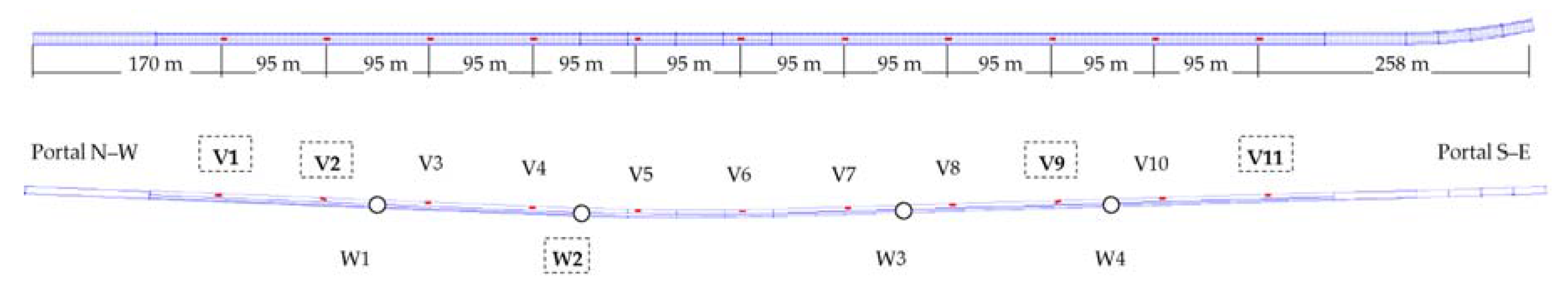
The tests included some configurations of switched on fans. After each change of the fans’ configuration, the air velocity was continuously monitored until it became stable. The additional air supply vents were closed. The tests summary is presented in
Table 4. The values of air velocity recorded by W2 gauge are taken into account; each value is averaged in the period of 15 min. Fans operation modes are described using the identifiers of switched on fans (according to the
Figure 1) and the working direction. Mode “0” means no fan was switched on.
At the first stage of the research the dependence of average air velocity on total fans thrust was checked. The data points from
Table 4 were plotted and the linear regression line was determined (
Figure 4).
The regression line should correspond to Equation (3). The value of
C coefficient is equal to 210 ± 23 [Ns
2/m
2]. As it can be seen the regression line fits the data points very well (
R2 = 0.964), but is shifted down. It is because a strong natural draught was observed during the measurements in the tunnel. Such natural airflow appears due to wind and natural stack effect. The value of this shift is 834 ± 206 N, what corresponds to pressure of 13.1 Pa (the area of the tunnel cross-section
A is equal to 63.6 m
2). This factor forcing natural airflow is called natural ventilation pressure—
NPV [
42].
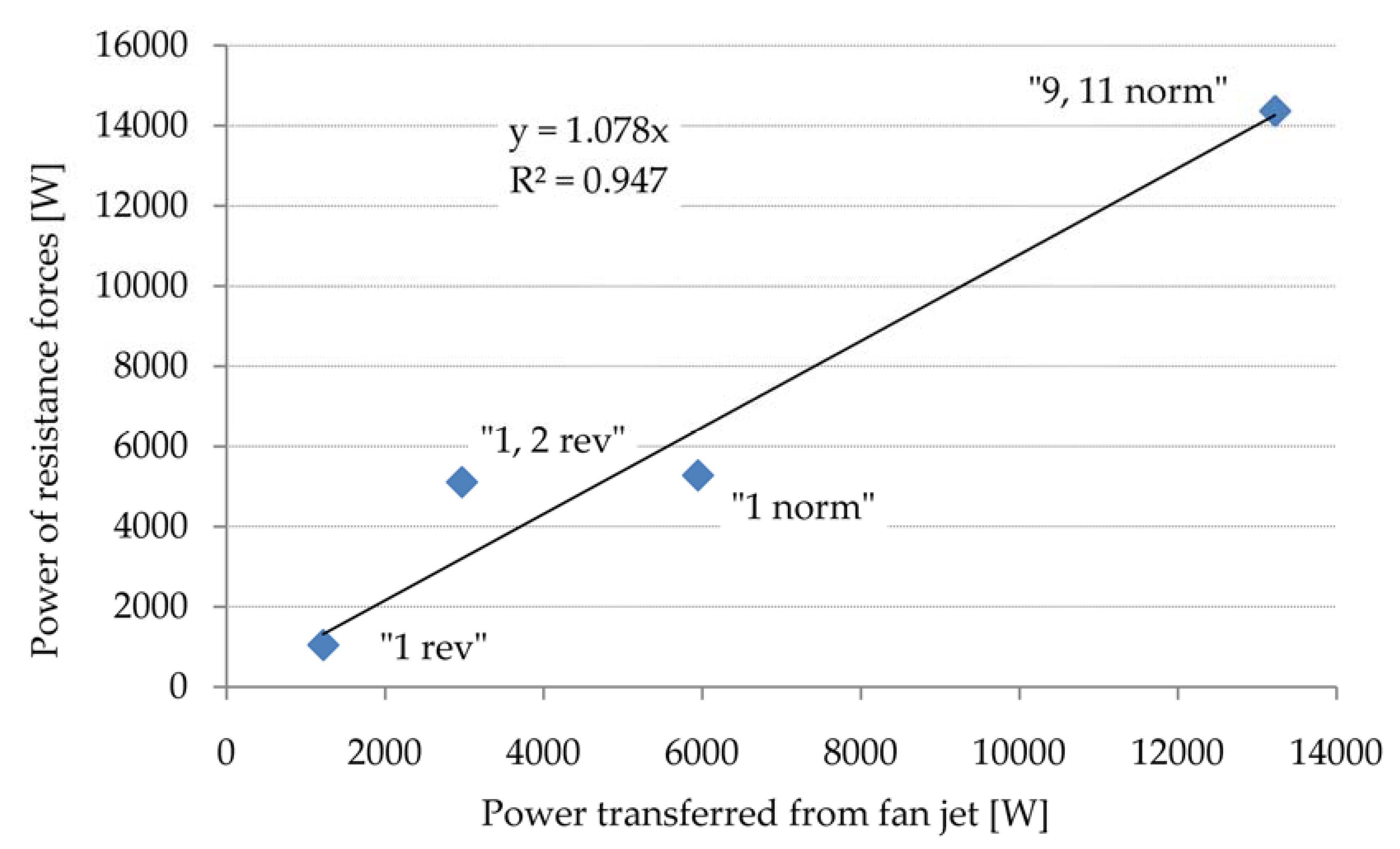
In the next step, there was an attempt to check the energy balance for all steady states with fans switched on. Natural ventilation pressure was taken into account as an additional energy source, which power (
PNPV) is expressed as:
Then according to Equation (12) the mechanical energy transferred from fan jet to air in the tunnel and energy loss due to flow resistance (Equation (13)) were calculated and compared. The energy generated by
NPV was added to the energy of fan jet for normal mode and added to the energy of resistance forces for reverse mode. The total mass of air taking part in the movement was roughly estimated as tunnel volume multiplied by air density. Values of constants
C and
NPV were taken from above regression data. The results are shown in
Figure 5. As both values are expected to be equal the equation of the trend line should be should be like y = x.
Due to rawness of the model there are significant discrepancies visible. But the regression line fits the points quite well, and the regression coefficient is very close to unity. It supports the presented conclusions on the energy balance of a fan jet. Finally, the whole kinetic energy provided by fans is dissipated, but the relevant temperature increase is immeasurable under conditions of the experiment in a real road tunnel.
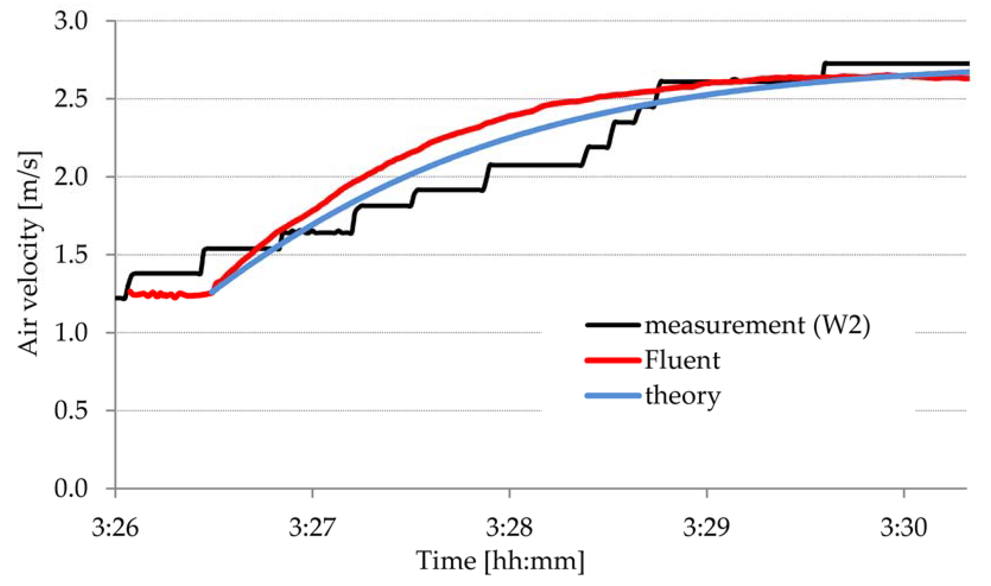
At the last stage of the presented study the transient processes were examined: the calculated air velocities were compared to the measured ones. Three cases were considered:
Fan no 1 was switched on in the normal mode—the air velocity started to increase from state “0” to state “1 norm”.
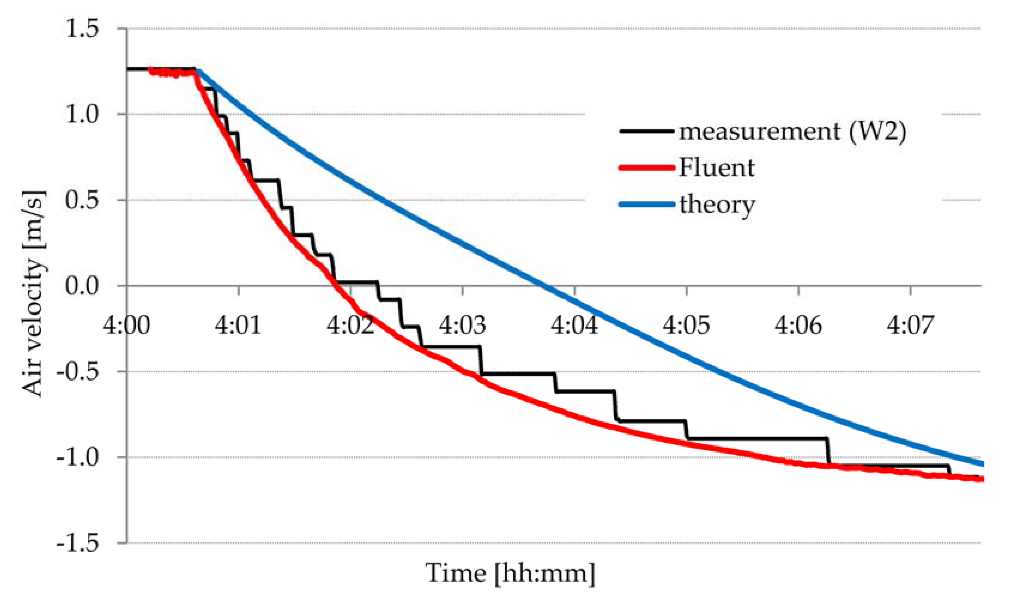
Fan no 1 was switched on in the reverse mode—the air velocity started to decrease from state “0”, changed its direction and finally reached state “1 rev”.
Fan no 1 was switched off from the normal mode—the air velocity started to decrease from state “1 norm” to state “0”.
These cases are shown in
Figure 6,
Figure 7 and
Figure 8. Additionally, the theoretic curves governed by Equation (4) are presented. The dynamic of air movement in all cases was determined here using the algorithm described by Equations (7) and (8). It is because of the permanent presence of natural draught in the tunnel, so the term expressed by
F was never equal to 0. The total mass of air taking part in the movement and values of constants
C and
NPV were adopted as previously and tuned in the allowed range.
It can be noted that the numerically calculated values fit the measurements rather well. A larger deviation can be observed for theoretical curves for cases 2 and 3. In the case 2 finally all curves converged. In turn, in case 3, the shape of all curves is similar, but the final value of theoretically calculated velocity is too high. These discrepancies might be caused by the simplicity of the theoretical model and the coarseness of estimation of total air mass moving in the tunnel. The reason of visible discrepancies between measurement and numerical model can be a result of variable conditions at tunnel portals. Value of dynamical pressure introduced into model, which related to wind impact was constant and was calculated taking into account the averaged measured wind velocity, meanwhile random gusts obviously took place during the experiment.
It can be observed that despite these discrepancies the measurements and both models led to the same time needed to reach the final steady state of airflow: 4 min in case 1, 6 min in case 2 and 5 min in case 3.
6. Conclusions and Discussion
The most important remark is that the time of the airflow relaxation is rather long—it is approximately a few minutes for all examined cases. While, as was mentioned in the Introduction section, the recommended time for achieving full capacity should not exceed 180 s [
8]. This delay might be very important when considering the management of smoke in emergency conditions. Therefore, the discussed issue should be taken into account when designing the operation pattern of the ventilation system. The suggested way is to switch on a bigger number of fans at the beginning, which will force the desired airflow quickly. Then some of fans could be switched off. As the disturbance of natural stratification of smoke and air should be avoided each of these cases should be independently analysed.
Some ideas based on Equation (15) can also be applied to improve the efficiency of kinetic energy exchange between fan jet and air volume in a tunnel. It would require fans with smaller outlet velocity but much bigger diameter to keep the needed momentum transfer rate (fan thrust). It is because the product of the area of a fan outlet and square of the outlet velocity should be the same. Under such assumptions the fan diameter is proportional to the inverse of outlet velocity. The lower the assumed outlet velocity, the lower the energy of fan jet is while the efficiency of the momentum transfer remains the same. However, this is limited by reasonable fans dimensions or fans number.
Because the dynamic of airflow in a tunnel strongly depends on tunnel length, cross-section area, inclination, curvature and properties of mounted fans the analyses similar to the presented ones should be ever carried out. The rough estimation of airflow relaxation time can be done according to presented algorithm (Equations (7) and (8)).
One should have in mind that in a case of fire outbreak the structure of airflow in a tunnel would be altered. The buoyancy forces, which depend on the fire power should be also taken into account. The properties of air such as density and viscosity would be different as well due to high temperature. More importantly, the fluid filling the tunnel bulk should be no longer be regarded as homogenous. However, despite the above remarks, the overall conclusions concerning airflow relaxation are expected to remain the same. This is because the main factors taken into account here keep their roles, unless extremely high fire power is considered (many vehicles on fire or fire of an HGV with a flammable load).
As every road tunnel has its own characteristics, this all would require deep consideration for each fire scenario additionally taking into account variable weather conditions. Only then, the appropriate emergency patterns for a fire ventilation system could be designed. But that is just the numerical analysis to be regarded as the most suitable tool for analysing the dynamic of airflow in tunnels. It particularly concerns more complex cases of tunnels with junctions and entrance ramps, where a simple model cannot by applied. Similarly, different fire locations and fire powers should be considered. However, one should have in mind that numerical models ought to be validated with real data, at least partially.


