Abstract
Short-term load forecasting is the basis of power system operation and analysis. In recent years, the use of a deep belief network (DBN) for short-term load forecasting has become increasingly popular. In this study, a novel deep-learning framework based on a restricted Boltzmann machine (RBM) and an Elman neural network is presented. This novel framework is used for short-term load forecasting based on the historical power load data of a town in the UK. The obtained results are compared with an individual use of a DBN and Elman neural network. The experimental results demonstrate that our proposed model can significantly ameliorate the prediction accuracy.
1. Introduction
In modern society, electrical energy has become the basic resource of national economic and social development, which is widely applied in various fields, such as power, lighting, chemistry, textile, communication, and broadcasting. With growing living standards and the fast development of electric power industry, better quality power supply has been requested. This means that power users need more economical and reliable electrical energy. The forms of electricity generation and consumption are changing all the time. Due to the non-storable character of electric energy, it is expected that the electricity supply and demand can be balanced as much as possible. Electricity generation needs to change along with electricity consumption; otherwise, the stability of the power system could be endangered [1]. In order to keep the balance of the electrical power network, a precise load prediction is essential. Load prediction can be categorized into four classes: ultra-short-term forecasting, short-term forecasting, medium-term forecasting, and long-term forecasting, based on the forecasting duration.
Short-term load forecasting is the basis of power system operation and analysis, referring to the power load prediction for the next few hours, one day, or several days. This load forecasting is beneficial for optimizing operation time of generating units, i.e., the starting and stopping time, and their output. A precise load forecast is helpful for minimizing the total consumption of the generating units [2]. Therefore, improving the accuracy of short-term load forecasting is crucial in the operation and management of the modern power system.
According to the forecasting models, approaches for load forecasting can be loosely categorized into statistical models and artificial intelligence models. Statistical models include regression analysis [3], Box–Jenkins models [4], Kalman filtering [5], autoregressive integrated moving average (ARIMA) [6], exponential smoothing [7], state space model [8], and so on. Artificial intelligence models include artificial neural networks (ANNs) [9], support vector machines (SVM) [10], data mining approaches [11,12], etc. Compared with statistical models, artificial intelligence models are usually more suitable for complex problems. Furthermore, hybridmodels [13], which integrate different models, have been studied to ameliorate the prediction effect. This method is designed to preserve the advantages of each individual model, and is shown to have good performance. The features of several common models are introduced in Table 1.

Table 1.
The features of several common models.
Among different kinds of prediction models, a deep belief network (DBN) [14] has shown promising performance. The deep belief network has a deep architecture that can represent multiple features of input patterns hierarchically with the pre-trained restricted Boltzmann machine (RBM). It has been widely used in many fields, such as image processing [15], dimensionality reduction [16], and classification tasks [17]. Previous research has shown that a DBN performs significantly better than shallow neural networks [18]. Compared with the shallow model, DBN can reveal the implicit characteristics of data from the bottom to the top.
In the last decade, numerous studies have been conducted using deep belief networks to perform time series data prediction [19]. For instance, Hu et al. [20] pre-trained a deep belief network using different pre-training models and investigated the difference between a DBN and a Stacked Denoising Autoencoder (SDA) when used as pre-training models. Qiu et al. [21] proposed an ensemble approach based on a DBN and Empirical Mode Decomposition (EMD) algorithm to forecast load time series. Adachi et al. [22] used samples from a D-Wave quantum annealing machine to estimate model expectations of Restricted Boltzmann Machines. Keyvanrad et al. [23] developed a new model named nsDBN that has different behaviors according to deviation of the activation of the hidden units from a fixed value. Meanwhile, the model has a variance parameter that can control the force degree of sparseness. Plahl et al. [24] explored a Sparse Encoding Symmetric Machine (SESM) to pre-train DBNs and applied this method to speech recognition. Ranzato et al. [25] described a novel and efficient algorithm to learn sparse representations, and compared it theoretically and experimentally with a Restricted Boltzmann Machine. Kamada et al. [26] proposed an adaptive structure learning method of a Restricted Boltzmann Machine (RBM), which can generate/annihilate neurons by a self-organized learning method according to input patterns. In addition, the adaptive DBN in the assembly process of a pre-trained RBM layer was also proposed. Papa et al. [27] applied a fast meta-heuristic approach called Harmony Search (HS) to fine-tune the parameters of a DBN. Kuremoto et al. [28] optimized the number of input (visible) and hidden neurons by means of the Particle Swarm Optimization (PSO) method, as well as the RBM learning rate. Torres et al. [29] developed a new approach which used an Apache Spark framework to load data in memory and deep learning methods as regressors to forecast electricity consumption. Quyang et al. [30] proposed a data-driven deep learning framework for power load forecasting. First, a Gumbel-Hougaard Copula model is used to model the tail-dependence between power load, electricity price, and temperature. Then, the tail-dependence is applied to a deep belief network for power load forecasting.
Although the DBN has been widely studied, as displayed by the aforementioned studies, to the best of our knowledge, focus is mainly on the training process of DBNs, more specifically, the training of RBMs. Research on the network structure of a DBN is rarely reported in the literature. After the pre-training stage of a DBN, the obtained parameters can be expanded for a multi-hidden layer neural network (MLNN). Generally, neural network models have two common types: Back Propagation (BP) neural networks and Elman neural networks. Compared with BP neural networks, Elman neural networks as a recurrent neural network have been proved to have better performance in time-series forecasting. In the last few decades, the Elman neural network model has been studied extensively for short-term electrical load forecasting [31]. For instance, the combination of an Elman network and wavelet is proposed to forecast a one-day-ahead electrical power load by considering the impact of temperature in Reference [32]. Similarly, in Reference [33], the authors investigated the short-term load forecasting problem via a hybrid quantized Elman neural network with the least number of quantized inputs, hourly historical load, hourly predicted target temperature, and time index. Despite the considerable research on Elman neural networks, these studies focus on shallow neural networks. Research on the combination of DBN and Elman neural networks for short-term load forecasting is rarely investigated. To fill in this research gap, this study proposed a new deep learning framework for short-term load prediction based on RBM and Elman neural networks.
The rest of the paper is organized as follows. Preliminary knowledge, including introductions to deep belief networks and Elman neural networks, is described in Section 2. Section 3 introduces the proposed Elman integrated deep learning framework. Experimental results are presented in Section 4, and Section 5 concludes this paper and identifies future studies.
2. Methodology
2.1. Deep Belief Network
The DBN is a deep neural network that consists of several layers of restricted Boltzmann machines (RBMs) and a layer of neural network (NN) [34]. The network structure of a typical DBN is shown in Figure 1.Traditional NN models adopt a gradient descent algorithm as the main training method, which is easily trapped in a local minimum value. When the NN structure becomes deep, this drawback becomes apparent because numerous network parameters need to be optimized. Initializing the network parameters to the greatest extent possible is a more sensible method to mitigate the local optimum dilemma. Consequently, in the search spaces, if the network parameters are initialized close to the optimal values, the opportunity to find out the global optimum will also greatly increase. With regard to DBNs, the training process consists of two components: a layer-wise pre-training process and a fine-tuning process. The former is applied to provide better initial values of the network parameters, and the latter is applied to search the optimal parameters based on the initial states of the network.
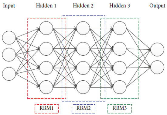
Figure 1.
Illustration of a typical DBN structure.
2.1.1. Pre-Training Process
The parameters of each hidden layer in a DBN can be initialized by the pre-training process, resulting in a better local optimum, or even the global optimal region. This process is obtained through an unsupervised greedy optimization algorithm by using the restricted Boltzmann machine (RBM).
A restricted Boltzmann machine (RBM) can learn a distribution from its input sample, which is a stochastic two-neural network [35]. The network generally consists of two different layers of nodes: visible nodes and hidden nodes. There are connections between nodes in different layers, while there are no connections between nodes in the same layer. Connections between nodes are symmetric and bidirectional. RBMs have been applied to generate models of various data types. A single RBM is shown in Figure 2.
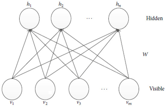
Figure 2.
Illustration of a typical RBM structure.
The RBM is an energy model. The energy function of visible layer and hidden layer is depicted as:
where and are the states of visible node and hidden node , respectively; and represent the bias between the visible layer and hidden layer; and is the connecting weight between them. A lower energy indicates that the network is in a more desirable state. This energy function is used to calculate the probability that is assigned to every possible pair of visible and hidden vectors:
where is the sum of over all possible configurations, and is used for normalization:
For binary state nodes and , the state of hidden node is set to 1 with probabilities:
where represents the logistic sigmoid function . The state of visible node is set to 1 with probability:
The training process of the RBM is described as follows. Firstly, a training sample is assigned to the visible nodes, and the is obtained. Then, the hidden nodes state is sampled according to probabilities. This process is repeated once more to update the visible and hidden nodes to produce the one-step “reconstructed” states and . The related parameters are updated as follows:
where represents the learning rate, and refers to the expectation of the training data. The above-mentioned expressions can be derived from the Contrastive Divergence (CD)algorithm.
2.1.2. Fine-Tuning
After pre-training, each layer of DBN is configured with initial parameters. Then the DBN starts fine-tuning the whole structure. Based on the loss function of the forecast data and the actual data, a gradient descent algorithm can be adopted to make a slight adjustment to the network parameters throughout the whole network, achieving the optimal states of the parameters. In this paper, the loss function is depicted as follows:
Where denotes the forecast data and denotes the actual data.
More generally, the DBN is a special BP neural network where the parameters of hidden layers are initialized by an RBM, instead of being randomly assigned.
2.2. Elman Neural Network
An Elman neural network is based on the BP neural network that adopts a connection layer to feedback the outputs from the hidden layer. It is a typical local recurrent neural network. The connection layer applies to memory the output value of the last step, which is then used as the input of the hidden layer. This can be considered as a step delay, which makes the Elman neural network sensitive to historical data, and thus, enables the network to have a dynamic memory function [36].
The basic Elman network is composed of an input layer, a connection layer, a hidden layer, and an output layer, as shown in Figure 3. The activation function of the hidden layer is nonlinear, e.g., the sigmoid function or the tan-sigmoid function. The activation function of the connection layer and the output layer is linear.
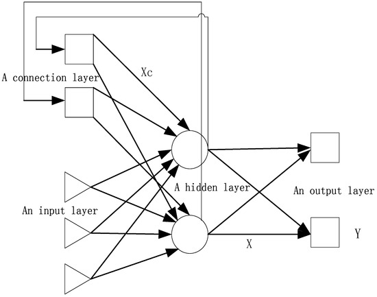
Figure 3.
Elman neural network structure.
In light of the Elman structure, the nonlinear relation of this model can be represented by the following mathematical equations:
where and are the output of the hidden layer and the input layer, respectively; and represent the output of the context layer and the output layer; is the activation function, which is usually a nonlinear sigmoid function; and is a pure linear activation function. W1, W2 and W3 are the connecting weights of the input layer to hidden layer, the connection layer to hidden layer, and the hidden layer to output layer, respectively; k is the kth iteration.
3. RBM-Elman Network
Compared with a BP neural network, which is a static mapping network, the Elman neural network appends an important feedback mechanism that behaves like a dynamic system. Therefore, it is more suitable for use as a time-series model. In this study, we propose a new deep learning framework based on RBM and Elman neural networks for short-term load prediction. The new deep learning framework is denoted as an RBM-Elman network.
3.1. RBM-Elman Optimization
Elman neural networks inherit some defects of BP neural networks. For example, a slow convergence rate and being easily trapped in local optima. These deficiencies are partly due to the randomly initialized parameters. Therefore, we proposed an RBM to initialize the weights and thresholds of Elman neural networks, by which we expected generalizability and the training speed of Elman neural networks to improve. The basic steps of our proposed method are described as follows, and Figure 4 shows the model implementation flowchart.
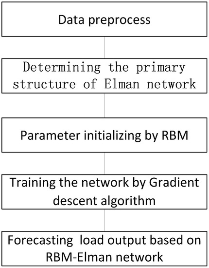
Figure 4.
The flowchart of the RBM-Elman model.
3.2. RBM-Elman Algorithm
The main steps of an RBM-Elman algorithm are discussed in turn below:
- determines the primary structure of an Elman neural network,
- applies RBMs to initialize the parameter of the hidden layer of Elman neural network,
- trains the Elman neural network using a gradient descent algorithm, and
- forecasts load output based on the trained network.
The significance of the new model is the initialization of connection weights and threshold using RBMs. This is expected to be helpful in improving the training speed and convergence, saving the network running time.
4. Case Studies
In order to validate the forecast performance of our proposed model, we describe a realistic case study of short-term load prediction in this section. First, the data set and model implementation are illustrated. Then, experimental results are demonstrated.
4.1. Data Set
The historical power load data of a town in the UK is employed to investigate the forecast effect of our proposed model. The chosen dataset is composed of 24 h of load data from 1 January 2014 to 31 December 2014. The whole dataset is further divided into two subsets: the training set and the testing set. In this study, about 80% of the whole dataset, i.e., the first 292 days, is chosen as the training set. The rest of data is applied to test the forecasting performance of the proposed model. Figure 5 shows an example of load data for June 2014.
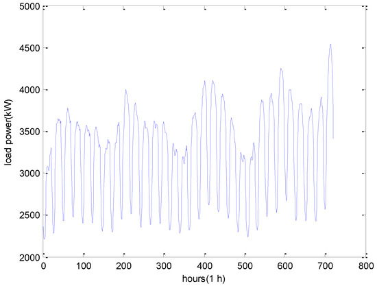
Figure 5.
Illustration of the load power in June 2014.
4.2. Model Implementation
4.2.1. Parameter Settings
As indicated above, the input data of the forecast model is the historical power load data. To construct the RBM-Elman model, the raw time-series data was transformed into a more suitable form. In this paper, we employed the state space reconstruction technique with the delay embedding theorem [37] to manipulate the raw data. The discrete time dynamic system was described as:
where represents a nonlinear vector valued function and represent the system state at time step . By the delay embedding theorem, it was supposed that the information of higher dimensional data could be compressed into the one-dimensional chaotic data. Therefore, the time series data was reconstructed as follows:
where represents the embedding dimension and represents time delay. Therefore, reconstructing time series turns into finding the optimal values of parameters and . For a given dataset, the false nearest neighbor method and mutual information function were applied to determine these two parameters [38]. In this study, was determined to be 10 and was determined to be 6, which were obtained using the utility functions false nearest and mutual in TISEAN toolbox [39]. Then, the reconstructed time series was generated, which is used to train the RBM-Elman neural network. Because of the number of nodes in input layer for the RBM-Elman model was determined by the dimension of reconstructed delay vectors, which is 10, the number of input nodes was also 10. In addition, the raw data was normalized into [0, 1] to accelerate the model training process.
Next, the trial and error method was employed to investigate the number of nodes in the hidden layer. The trial and error results of Elman model are illustrated in Figure 6. From the Figure, we can observe that the mean absolute percentage error (MAPE) index of the model achieved optimal performance when the number was 24. Hence, the structure of optimal policy for Elman neural network is 10-24-1, and the number of context layer nodes was also 24.
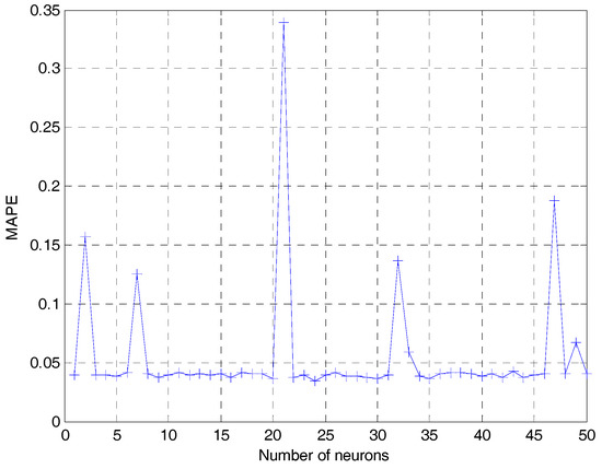
Figure 6.
The trial and error results of Elman model.
In the end, for this neural network, the activation functions in the hidden layer and the output layer were the common tan-sigmoid and pure linear function, respectively. The diagram of the model is illustrated in Figure 7.
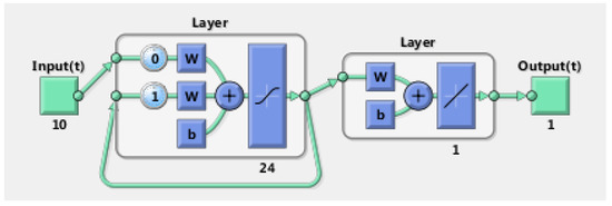
Figure 7.
The structure of Elman neural network.
4.2.2. Model Evaluation
To examine the performance of our proposed model, two metrics were calculated to evaluate the error of output power prediction, including MAPE and mean squared error (MSE), which are frequently used in the literature. The MAPE and MSE are defined as:
where denotes the number of forecast sample, represents the actual value at time instance , and is the predicted value.
4.3. Experimental Results
The proposed RBM-Elman model was employed for use in a short-term load prediction. For comparison purposes, a DBN model was designed to perform the short-term load prediction with the same dataset. A typical three-layer Elman neural network was also employed to demonstrate the validity of our proposed model. The results obtained by each prediction method are illustrated in Table 2. Furthermore, the forecasting results by RBM-Elman model for test data are illustrated in Figure 8. For a better visualization, the results of seven consecutive days are also illustrated in Figure 9. The forecasting results of seven consecutive days by the DBN model and Elman model are illustrated in Figure 10 and Figure 11, respectively.
Table 2.
Forecast results by different models.
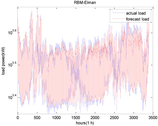
Figure 8.
The forecast results using RBM-Elman model for test data.
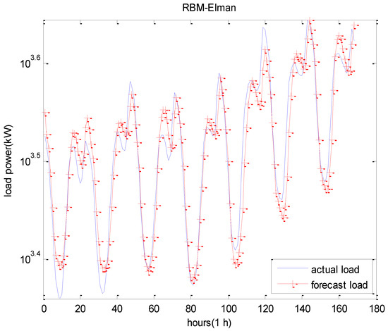
Figure 9.
The forecast results of seven consecutive days using RBM-Elman model.
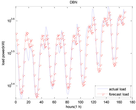
Figure 10.
The forecast results of seven consecutive days using DBN model.
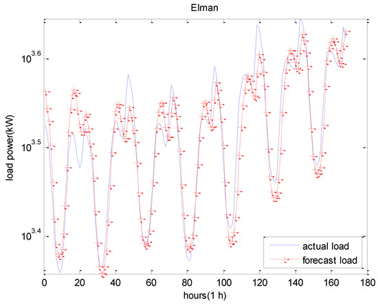
Figure 11.
The forecast results of seven consecutive days using Elman model.
The tabular overviews of the results are presented in Table 2. Amongst them, the MAPE of the RBM-Elman network was the minimum, which was 0.0346. The MAPE of the DBN was 0.0381. From Table 2, we can see that the forecast performance of our proposed RBM-Elman prediction model was better than other models. Meanwhile, it had a shorter computing time. From the above Figures, it is also evident that our proposed method provided a better match of actual load and forecasted load.
In order to further demonstrate the forecast performance of our proposed method, we decomposed the dataset based on different seasons. Each season’s dataset is split into the usual 80–20% training-test sets structure. Then our proposed method is applied to examine them. The forecast results of different seasons by RBM-Elman model are given in Table 3. From the results, we can see that the RBM-Elman model achieved good forecasting precision for four seasons. In addition, the forecast results of spring and autumn are better than those of summer and winter. This may be due to the change of temperature in summer and winter seasons.
Table 3.
Forecast results of different seasons by RBM-Elman model.
5. Conclusions
In the competitive electricity market, an accurate electricity load forecast is necessary. In this study, a deep learning framework based on RBM and Elman neural networks was presented. To verify the effectiveness of our proposed model, the proposed model was compared with an individual use of the DBN and Elman neural networks. The results of these experiments demonstrate that our proposed model achieved the best forecasting precision and had a shorter computing time.
In future studies, we would first like to examine our method on more complex datasets. Second, the hyper-parameters of neural networks were fine-tuned by the back-propagation method, which makes it easy to fall into local optima. Thus, we would like to apply advanced evolutionary algorithms [40,41,42,43] to lightly adjust those hyper-parameters to improve the performance of neural networks even further. Lastly, other improvements of the deep believe network for load predication will also be considered.
Author Contributions
X.Z. built the model; X.Z. and R.W. designed and realized the algorithm; T.Z., Y.Z. and Y.L. contributed to the application and provided helpful advice; and X.Z. and R.W. wrote the paper.
Funding
This work was supported by the Distinguished Natural Science Foundation of Hunan Province (No. 2017JJ1001) and the National Natural Science Foundation of China (No. 61773390, 71571187).
Conflicts of Interest
The authors declare no conflict of interest.
Abbreviations
| ANN | Artificial Neural Network |
| ARIMA | Autoregressive Integrated Moving Average |
| BP | Back Propagation |
| CD | Contrastive Divergence |
| DBN | Deep Belief Network |
| EMD | Empirical Mode Decomposition |
| HS | Harmony Search |
| MAE | Mean Squared Error |
| MAPE | Mean Absolute Percentage Error |
| NN | Neural Network |
| PSO | Particle Swarm Optimization |
| RBM | Restricted Boltzmann Machine |
| SDA | Stacked Denoising Autoencoder |
| SESM | Sparse Encoding Symmetric Machine |
| SVM | Support Vector Machines |
| TISEAN | Time Series Analysis |
References
- Jiang, P.; Liu, F.; Song, Y. A hybrid forecasting model based on date-framework strategy and improved feature selection technology for short-term load forecasting. Energy 2017, 119, 694–709. [Google Scholar] [CrossRef]
- Chen, Y.; Luh, P.B.; Rourke, S.J. Short-term load forecasting: Similar day-based wavelet neural networks. In Proceedings of the 2008 7th World Congress on Intelligent Control and Automation, Chongqing, China, 25–27 June 2008; pp. 3353–3358. [Google Scholar]
- Chen, C.; Zhou, J.N. Application of Regression Analysis in Power System Load Forecasting. Adv. Mater. Res. 2014, 960–961, 1516–1522. [Google Scholar] [CrossRef]
- Vähäkyla, P.; Hakonen, E.; Léman, P. Short-term forecasting of grid load using Box-Jenkins techniques. Int. J. Electr. Power Energy Syst. 1980, 2, 29–34. [Google Scholar] [CrossRef]
- Shankar, R.; Chatterjee, K.; Chatterjee, T.K. A Very Short-Term Load forecasting using Kalman filter for Load Frequency Control with Economic Load Dispatch. J. Eng. Sci. Technol. Rev. 2012, 5, 97–103. [Google Scholar]
- Wei, L.; Zhen-gang, Z. Based on time sequence of ARIMA model in the application of short-term electricity load forecasting. In Proceedings of the International Conference on Research Challenges in Computer Science, Shanghai, China, 8–29 December 2009; pp. 11–14. [Google Scholar]
- Li, X.; Chen, H.; Gao, S. Electric power system load forecast model based on State Space time-varying parameter theory. In Proceedings of the International Conference on Power System Technology, Hangzhou, China, 24–28 October 2010; pp. 1–4. [Google Scholar]
- Christiaanse, W.R. Short-term load forecasting using general exponential smoothing. IEEE Trans. Power Appar. Syst. 2007, 900–911. [Google Scholar] [CrossRef]
- Lee, K.Y.; Cha, Y.T.; Park, J.H. Short-term load forecasting using artificial neural networks. IEEE Trans. Power Syst. 2014, 7, 124–132. [Google Scholar] [CrossRef]
- Li, G.; Cheng, C.T.; Lin, J.Y. Short-Term Load Forecasting Using Support Vector Machine with SCE-UA Algorithm. In Proceedings of the International Conference on Natural Computation, Haikou, China, 4–27 August 2007; pp. 290–294. [Google Scholar]
- Martínez-Álvarez, F.; Troncoso, A.; Asencio-Cortés, G.; Riquelme, J.C. A Survey on Data Mining Techniques Applied to Electricity-Related Time Series Forecasting. Energies 2015, 8, 13162–13193. [Google Scholar] [CrossRef]
- Duque-Pintor, F.; Fernández-Gómez, M.; Troncoso, A. A New Methodology Based on Imbalanced Classification for Predicting Outliers in Electricity Demand Time Series. Energies 2016, 9, 752. [Google Scholar] [CrossRef]
- Kavousi-Fard, A.; Kavousi-Fard, F. A new hybrid correction method for short-term load forecasting based on ARIMA, SVR and CSA. J. Exp. Theor. Artif. Intell. 2013, 25, 559–574. [Google Scholar] [CrossRef]
- Hinton, G.E.; Osindero, S.; Teh, Y.W. A fast learning algorithm for deep belief nets. Neural Comput. 2006, 18, 1527–1554. [Google Scholar] [CrossRef] [PubMed]
- Cheng, M. The cross-field DBN for image recognition. In Proceedings of the IEEE International Conference on Progress in Informatics and Computing, Nanjing, China, 8–20 December 2015; pp. 83–86. [Google Scholar]
- Arsa, D.M.S.; Jati, G.; Mantau, A.J. Dimensionality reduction using deep belief network in big data case study: Hyper spectral image classification. In Proceedings of the International Workshop on Big Data and Information Security, Jakarta, Indonesia, 18–19 October 2016; pp. 71–76. [Google Scholar]
- Sun, S.; Liu, F.; Liu, J. Web Classification Using Deep Belief Networks. In Proceedings of the 2014 IEEE 17th International Conference on Computational Science and Engineering, Chengdu, China, 19–21 December 2014; pp. 768–773. [Google Scholar]
- Chao, J.; Shen, F.; Zhao, J. Forecasting exchange rate with deep belief networks. In Proceedings of the International Joint Conference on Neural Networks, San Jose, CA, USA, 31 July–5 August 2011; pp. 1259–1266. [Google Scholar]
- Kuremoto, T.; Kimura, S.; Kobayashi, K. Time series forecasting using a deep belief network with restricted Boltzmann machines. Neurocomputing 2014, 137, 47–56. [Google Scholar] [CrossRef]
- Hu, Z.; Xue, Z.Y.; Cui, T. Multi-pretraining Deep Neural Network by DBN and SDA. In Proceedings of the International Conference on Computer Engineering and Information Systems, Kunming, China, 21–23 September 2013. [Google Scholar]
- Qiu, X.; Ren, Y.; Suganthan, P.N. Empirical Mode Decomposition based ensemble deep learning for load demand time series forecasting. Appl. Soft Comput. 2017, 54, 246–255. [Google Scholar] [CrossRef]
- Adachi, S.H.; Henderson, M.P. Application of Quantum Annealing to Training of Deep Neural Networks. arXiv, 2015; arXiv:1510.06356. [Google Scholar]
- Keyvanrad, M.A.; Homayounpour, M.M. Normal sparse Deep Belief Network. In Proceedings of the International Joint Conference on Neural Networks, Killarney, Ireland, 12–17 July 2015; pp. 1–7. [Google Scholar]
- Plahl, C.; Sainath, T.N.; Ramabhadran, B. Improved pre-training of Deep Belief Networks using Sparse Encoding Symmetric Machines. In Proceedings of the International Conference on Acoustics, Speech and Signal Processing, Kyoto, Japan, 25–30 March 2012; pp. 4165–4168. [Google Scholar]
- Ranzato, M.A.; Boureau, Y.L.; Lecun, Y. Sparse feature learning for deep belief networks. In Proceedings of the International Conference on Neural Information Processing Systems, British, DC, Canada, 7–10 December 2009; Curran Associates Inc.: Red Hook, NY, USA, 2007; pp. 1185–1192. [Google Scholar]
- Kamada, S.; Ichimura, T. Fine tuning method by using knowledge acquisition from Deep Belief Network. In Proceedings of the International Workshop on Computational Intelligence and Applications, Hiroshima, Japan, 5 January 2017; pp. 119–124. [Google Scholar]
- Papa, J.P.; Scheirer, W.; Cox, D.D. Fine-tuning Deep Belief Networks using Harmony Search. Appl. Soft Comput. 2015, 46, 875–885. [Google Scholar] [CrossRef]
- Kuremoto, T.; Kimura, S.; Kobayashi, K. Time Series Forecasting Using Restricted Boltzmann Machine. In Emerging Intelligent Computing Technology and Applications; Springer: Berlin/Heidelberg, Germany, 2012; pp. 17–22. [Google Scholar]
- Torres, J.; Fernández, A.; Troncoso, A.; Martínez-Álvarez, F. Deep learning-based approach for time series forecasting with application to electricity load. In Proceedings of the International Work-Conference on the Interplay between Natural and Artificial Computation, Corunna, Spain, 19–23 June 2017; Springer: Cham, Switzerland, 2017; pp. 203–212. [Google Scholar]
- Ouyang, T.; He, Y.; Li, H.; Sun, Z.; Baek, S. A Deep Learning Framework for Short-term Power Load Forecasting. arXiv, 2017; arXiv:1711.11519. [Google Scholar]
- Liang, Y. Application of Elman Neural Network in Short-Term Load Forecasting. In Proceedings of the International Conference on Artificial Intelligence and Computational Intelligence, Sanya, China, 23–24 October 2010; pp. 141–144. [Google Scholar]
- Kelo, S.; Dudul, S. A wavelet Elman neural network for short-term electrical load prediction under the influence of temperature. Int. J. Electr. Power Energy Syst. 2012, 43, 1063–1071. [Google Scholar] [CrossRef]
- Li, P.; Li, Y.; Xiong, Q. Application of a hybrid quantized Elman neural network in short-term load forecasting. Int. J. Electr. Power Energy Syst. 2014, 55, 749–759. [Google Scholar] [CrossRef]
- Zhang, X.; Wang, R.; Zhang, T. Short-term load forecasting based on an improved deep belief network. In Proceedings of the International Conference on Smart Grid and Clean Energy Technologies, Chengdu, China, 19–22 October 2016; pp. 339–342. [Google Scholar]
- Zhang, X.; Wang, R.; Zhang, T. Effect of Transfer Functions in Deep Belief Network for Short-Term Load Forecasting. In International Conference on Bio-Inspired Computing: Theories and Applications; Springer: Singapore, 2017; pp. 511–522. [Google Scholar]
- Zhang, X.; Wang, R.; Zhang, T. Short-Term Forecasting of Wind Power Generation Based on the Similar Day and Elman Neural Network. In Proceedings of the 2015 IEEE Symposium Series on Computational Intelligence, Cape Town, South Africa, 7–10 December 2015; pp. 647–650. [Google Scholar]
- Takens, F. Detecting strange attractors in turbulence. In Dynamical Systems and Turbulence, Warwick 1980; Springer: Berlin, Germany, 1981; pp. 366–381. [Google Scholar]
- Hegger, R.; Kantz, H.; Schreiber, T. Practical implementation of nonlinear time series methods: The TISEAN package. Chaos 1999, 9, 413–435. [Google Scholar] [CrossRef] [PubMed]
- Nonlinear Time Series Analysis (TISEAN). Available online: https://www.mpipks-dresden.mpg.de/tisean/ (accessed on 5 June 2018).
- Wang, R.; Purshouse, R.C.; Fleming, P.J. Preference-inspired Co-evolutionary Algorithms for Many-objective Optimization. IEEE Trans. Evolut. Comput. 2013, 17, 474–494. [Google Scholar] [CrossRef]
- Wang, R.; Ishibuchi, H.; Zhou, Z.; Liao, T.; Zhang, T. Localized weighted sum method for many-objective optimization. IEEE Trans. Evolut. Comput. 2018, 22, 3–18. [Google Scholar] [CrossRef]
- Wang, R.; Zhang, Q.; Zhang, T. Decomposition based algorithms using Pareto adaptive scalarizing methods. IEEE Trans. Evolut. Comput. 2016, 20, 821–837. [Google Scholar] [CrossRef]
- Li, K.W.; Wang, R.; Zhang, T.; Ishibuchi, H. Evolutionary Many-objective Optimization: A Comparative Study of the State-of-the-Art. IEEE Access. 2018, 6, 26194–26214. [Google Scholar] [CrossRef]
© 2018 by the authors. Licensee MDPI, Basel, Switzerland. This article is an open access article distributed under the terms and conditions of the Creative Commons Attribution (CC BY) license (http://creativecommons.org/licenses/by/4.0/).