Article

Study of Power Quality at the Point of Common Coupling of a Low Voltage Grid and a Distributed Generation System of 7.8 kWp in a Tropical Region

1
Facultad de Ingeniería, Universidad de Ibagué, Ibagué 730001, Colombia
2
School of Engineering, Universidade Estadual Paulista (UNESP) Câmpus Guaratinguetá, Guaratinguetá 01049-010, Brazil
*
Author to whom correspondence should be addressed.
Energies 2018, 11(6), 1539; https://doi.org/10.3390/en11061539
Submission received: 25 May 2018 / Revised: 6 June 2018 / Accepted: 7 June 2018 / Published: 13 June 2018
(This article belongs to the Special Issue Building renewable energy and thermal energy storage system 2018)

Abstract

:
In this paper we analyze an experimental 1000 kWh/month distributed generation system in a tropical region connected to a point of common coupling in a low voltage grid that was characterized according to NTC 5001. This photovoltaic system has 7.8 kWp and uses 30 polycrystalline silicon-panels of 260 Wp each. Its maximum energy produced was 850 kWh/month, equivalent to 72.65% of the installed capacity. Finally, there was an increase of 2% with respect to the minimum voltage value that was recorded. The voltage unbalance decreases between 3.5 and 70% and voltage harmonics in each line increased by 7% on line U1, 0.8% on U2, 3% on U3 and current harmonics have a 22% increase. Likewise, the total active and reactive power were increased by 58% and 42% respectively, and the thermography study allowed to establish a temperature increase at the point of common coupling of 7.5%. Therefore, it is expected that this paper can serve as a reference for the application of Colombian law 1715 in solar energy.

1. Introduction

In response to the increase in energy demand and environmental restrictions on greenhouse gas emissions around the world, attention is now focused on renewable energy sources. Solar energy is considered an unlimited resource, so it could contribute to reduce the use of fossil fuels and their negative impacts. Moreover, it is considered more environmentally-friendly [1], safer, noise-free and easy to install [2]. Photovoltaic systems (PV) are manufactured using semiconductor materials such as silicon, which converts the incident radiation into electricity. This process is carried out directly and instantaneously, without complicated mechanical components [3] with maximum efficiencies reached in the range of 12–15% [4], in the case of commercial polycrystalline silicon cells.
Likewise, the PV industry and the market have grown rapidly in recent years, the main reason being the reduction of the generation costs and government policies that promote the introduction of PV systems connected to the grid. However, this growth has not been followed by developments in the field of failure diagnosis, monitoring and detection in PV systems, particularly in power outputs smaller than 25 kWp [5], a procedure that allows one to establish the state of a PV installation, the efficiency with which it is operating, as well as its behavior against climatic variables, such as ambient temperature, solar radiation and wind speed.
The International Energy Outlook (IE) indicates that energy consumption will increase by more than 28% in 2015 (6.06 × 1026 kJ) to 2040 (7.76 × 1026 kJ) and predicts that there will be a significant increase in the consumption of coal reserves in the next 20 years. This institution suggests that, in order to achieve a contribution to global energy demand and a significant impact on pollution reduction, renewable energy sources should grow in such a way that, by the year 2050 they will become more than half of the world’s energy needs [6]. According to the Renewable Energy police Network for the 21st Century (REN21), the contribution of renewable energy to global energy generation is 16%. The so-called new renewable energies, which include photovoltaic generation, contribute 0.6% [7].
It must be added that interconnected photovoltaic systems are being used as a complement to conventional energy generation in many countries [8,9]. Applications range from a small power generation in remote areas in the past 25 years to the installation of centralized stations with large photovoltaic generation capacity scale. In recent years, a great interest in urban consumers has been generated as a distributed generation application, where plants with small generation capacity are installed on the roofs of buildings or residences within the Building Integrated Photovoltaic Systems (BIPVS) concept. Nowadays, there is a variety of hybrid energy solutions for building applications [10,11,12,13], and especially ones with the integration of photovoltaics [14,15,16]. Their implementation mostly depends on the climate, geographical location, building type and on the availability of the energy resources on site. Despite the promising potential, one of the most important problems of PV systems is the dimensioning of its components, because, if a PV system is not correctly dimensioned, it does not work as expected [17].
Therefore, the sizing of grid-connected photovoltaic systems (GCPV) involves two main procedures, namely the technical sizing procedure and the economic sizing to determine the expected technical performance indicators and the economic performance indicator of the proposed system. In technical terms, the estimation of the energy produced by a GCPV is a widely studied concept [18,19,20,21]; we can find, based on various approaches to design-based software recently introduced, [22] methods and models for simulation to simplified calculation methods [23,24].
Currently there are online calculation methods that web pages of different organisms display, such as Joint Research Center (JRC) [25]. The design of the photovoltaic system connected to the low voltage grid (GCPV) of 7.8 kWp in this case of study was carried out following the recommendations by [26,27,28] with regard to the system evaluation, studies have been carried out in Europe and worldwide on the performance of photovoltaic systems operating outdoors as reported by [29,30,31,32,33,34,35].
On the behavior of the power quality at the point of common coupling (the low voltage network and a distributed generation system), many authors propose some possible solutions. Marnay [36], proposed a control strategy to control the voltage imbalance, the total harmonic distortion and the voltage gaps or SAGS, caused by large non-linear and unbalanced loads. Li et al. [37], suggested the use of a series-parallel converter to control the voltage imbalance and the current demand in the case of a fault in the network. A converter consisting of three single-phase inverters to control unbalanced and non-linear loads is proposed by [38,39]. Papadimitriou et al. [40] suggest that the imbalance of power, during the transition of the micro-grid from the mode connected to the disconnected can be restricted with a fuzzy and Zamani control et al. [41] proposed a closed-loop control strategy that allows the micro-grid to maintain a good power quality without changing the modes.
Although Latin America has a high potential for the use of photovoltaic energies [42], it lacks such studies. The performance evaluation of photovoltaic systems involves the calculation of the following parameters: annual energy generation, reference performance, final yield, system losses, loss of cell temperature, photovoltaic module efficiency, capacity factor and yield ratio among others [32]. The results obtained provided useful information to policymakers and organizations interested in the actual performance of grid-connected photovoltaic systems in a region or country [43].
Colombia has abundant natural resources, including a high-water potential, gas, coal, wind resources, solar energy and biomass. It is also located in an area of high geological activity that would make geothermal exploitation possible. One of the main difficulties is the lack of detailed information on the true potential of non-conventional renewable energy sources.
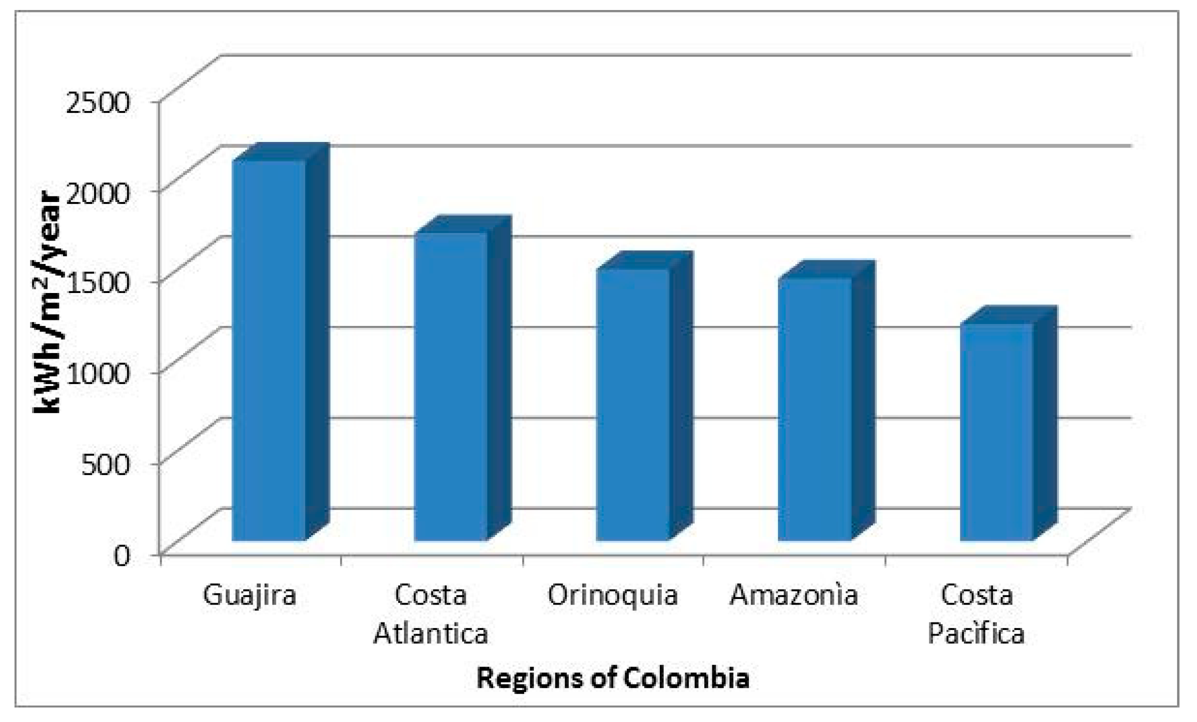
In general, the whole territory of Colombia has a good solar energy potential, with a daily average insolation of around 4.5 kWh/m2 (La Guajira Peninsula, with an average value of 2.200 kWh/m2/year can be highlighted) (Figure 1). Although Colombia has favorable legislation for alternative energies, the costs of implementation of photovoltaic systems compared to other energy sources remain high, with current costs of 2100 USD/kWp, only exceeded by geothermal generation at 2200 USD/kWp and higher than hydroelectric power plants with costs of 1300 USD/kWp, coal-fired power plants of 800 USD/kWp, thermoelectric plants with combined cycle gas with 900 USD/kWp, wind power plants at 1200 USD/kWp and cogeneration 500 USD/kWp. However, due to the low operation and maintenance costs of photovoltaic systems, these can surpass coal-fired power plants and combined-cycle gas-fired thermoelectric plants, making them an excellent alternative to be included in the Colombian energy matrix.
In 2014, Colombian government signed law 1715 which established the legal framework for the promotion and exploration of non-conventional energy sources, mainly from renewable sources, the promotion of investments, research and development of clean technologies in energy production. Experimental studies are needed to solve the problems of voltages caused by photovoltaic systems, since experimental data can show the actual behavior of the system.
Thus, all the technical problems (voltage, power, synchronicity, flicker and frequency) originating at the point of common coupling between the grid and the photovoltaic system should be thoroughly studied before its implementation. In this paper an evaluation of a photovoltaic system of 7.8 kWp, connected to a point of common coupling of a low-voltage grid, located in the city of Ibagué (Colombia) was carried out. Besides that, in this paper we present the behavior of the power quality at the common point of connection between a distributed generation system and a low voltage grid in a tropical region. This work is organized as follows: Section 2 describes the system and shows the evaluation parameters based on standards for Colombia. Section 3 explains the methodology of Colombian Technical Standard NTC 5001 for measurements in the energy quality studies. Following this, we present the instruments for the measurement in Section 4. Section 5 summarizes our results (system efficiency, power quality and thermography analysis), while Section 6 offers the conclusions.

2. Description of the Photovoltaic System Connected to the Low Voltage Grid

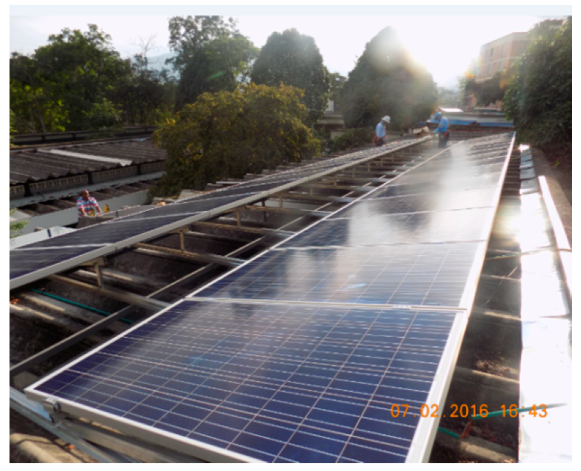
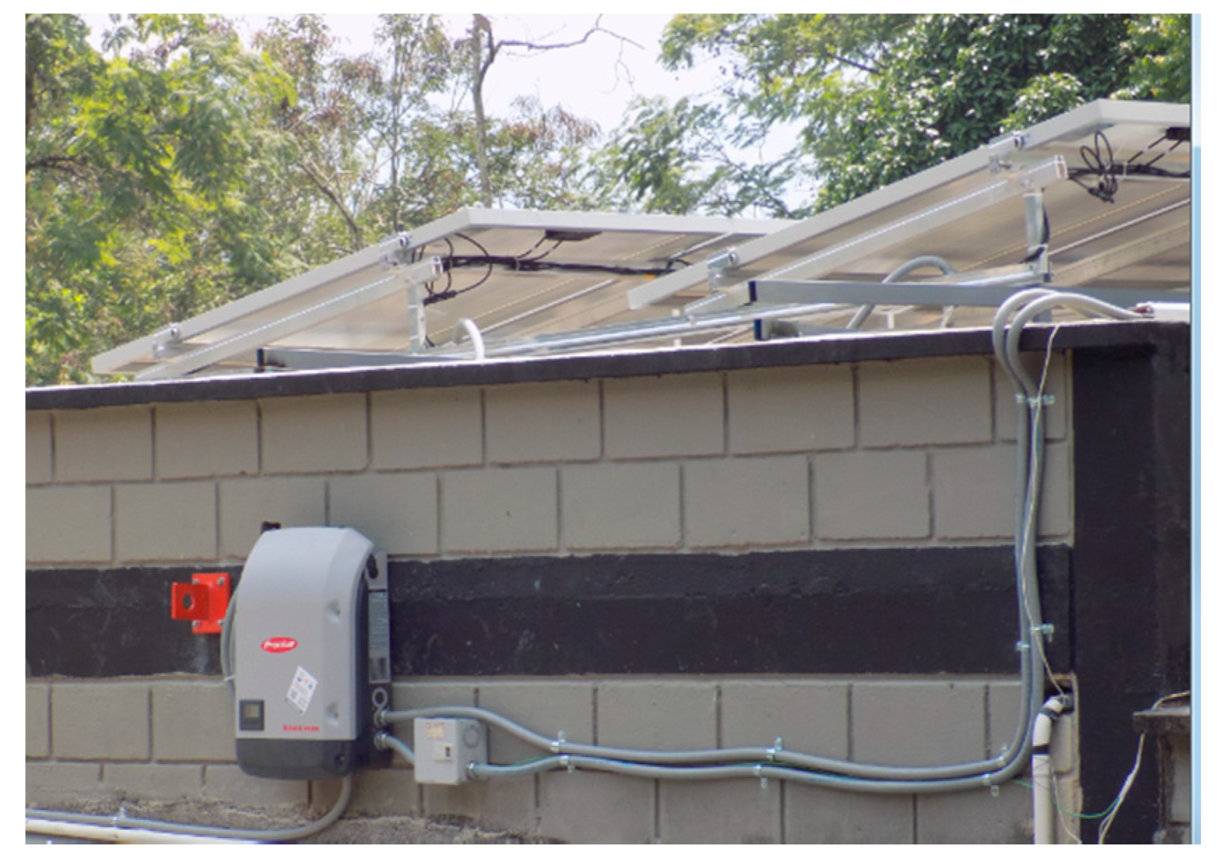
The experimental photovoltaic system has operated from February 2016 to date. It is located in block 3 at the Universidad de Ibagué at 1285 above sea level, latitude 4°26′54″ N, longitude 75°11′56″ W. The structure is made of I-beams of AISI 1045 steel, whose slope was calculated to be 12.3°, as shown in Figure 2, The system consists of 30 panels tilted at a fixed angle of 14° and oriented towards the north with an azimuth of 4°, it is divided into three modules with 10 IBC PolySol 260-CS polycrystalline silicon panels each (Colombinvest, Bogotá, Colombia, Table 1), which are connected in series covering an area of 49.1 m2. A Fronius Primo 7.6-1 inverter (Colombinvest, Bogotá, Colombia, 
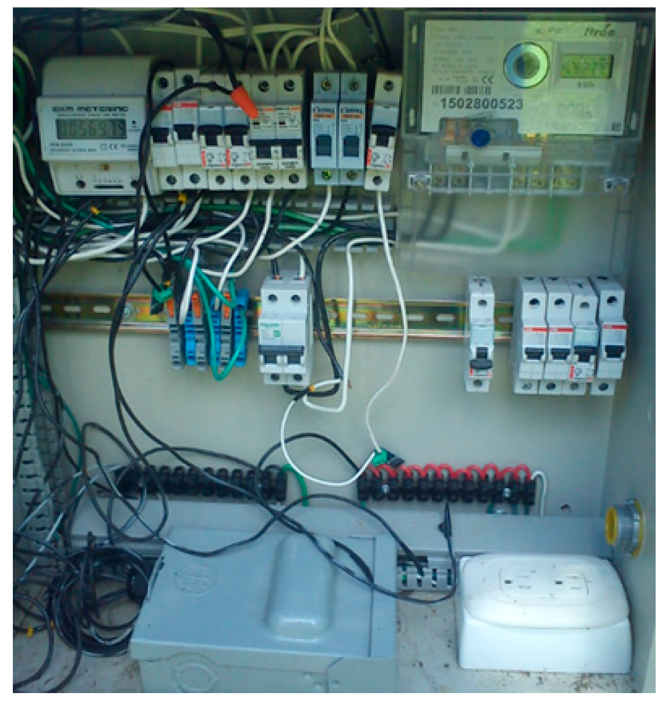
Table 2) with a rated maximum efficiency of 96.9% and maximum AC power of 7600 W is also part of the circuit, as well as the Itron ACE300 bidirectional counter (Colombinvest, Bogotá, Colombia), which measures the data about the total energy generation.
Moreover, the sizing ratio, which represents the ratio between the PV array installed capacity and the inverter capacity, in the present case, is 1.0. Data is recorded in 1 min intervals and processed by a computer. Solar radiation, wind speed and ambient temperature were provided by an automatic Meteorological Station (100 m away from the PV system) at the Universidad de Ibagué, Colombia.

2.1. Performance Parameters

In order to evaluate the performance of a photovoltaic system connected to the low voltage grid, parameters of the IEC 61724 standard are taken as a reference: output energy, yields (Reference, Array, Final), array and system losses, Efficiencies (Array, System, Inverter) [29,30,31,32,33,34,35]. These standardized performance parameters are relevant because they provide a basis by which grid-connected photovoltaic systems can be compared under various operating conditions [29].

2.2. System Efficiency

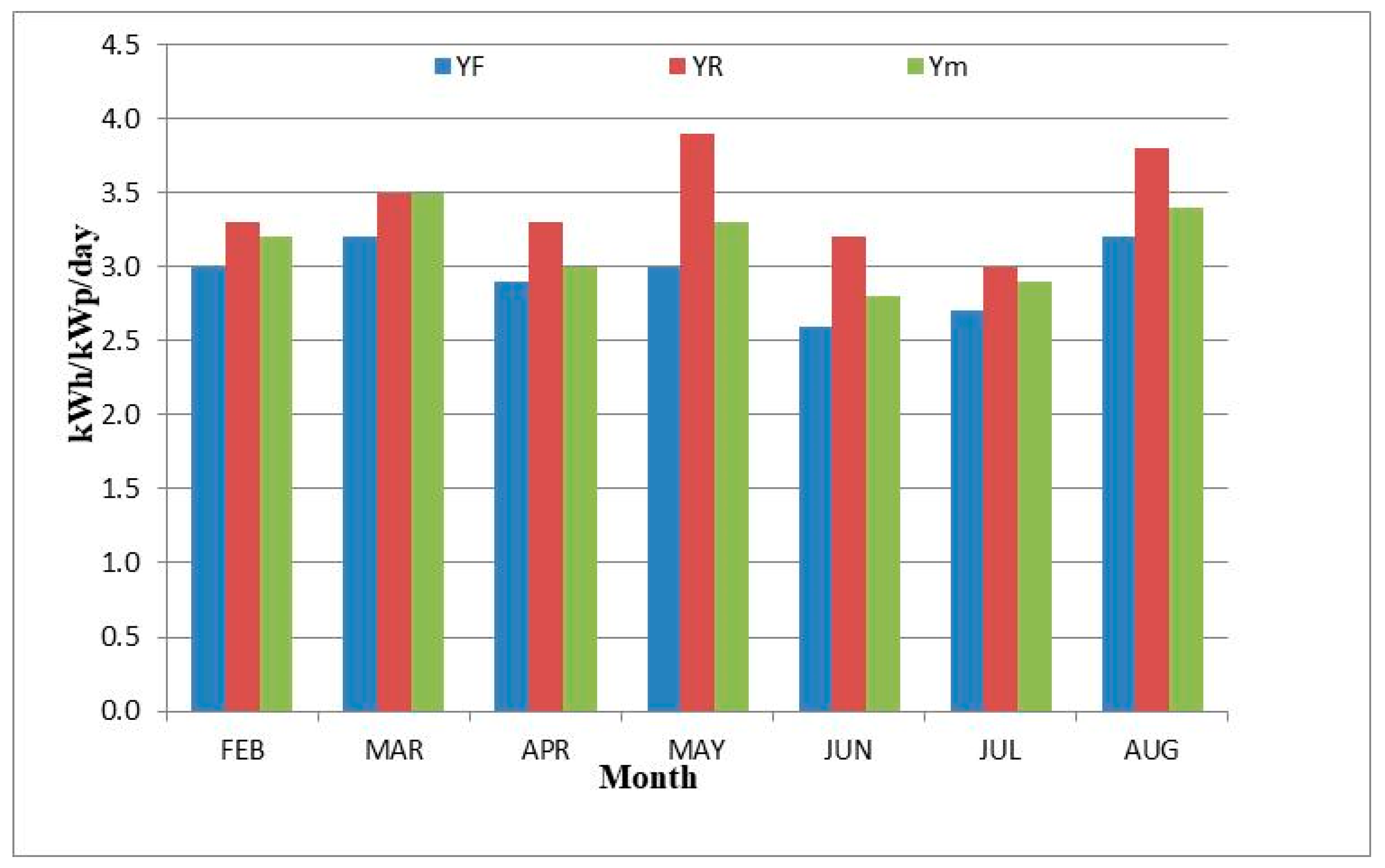
The yields indicate the actual operation of the modules relative to their rated capacity; they can be classified into three types: array performance (Ym), final (YF) and reference (YR) [29]. The array performance (Ym) is defined as the output direct current (DC) of the photovoltaic array over a period of time, divided by the nominal power. Other authors represent it as the time, measured in kWh/kWp, that the photovoltaic modules must operate at their nominal power to generate the energy produced [44]. It is represented by Equation (1):
Y m = E D P P V ( kWh kW p )
where ED is the energy output of the photovoltaic module in (kWh), and PPV the nominal power of the array in kWp.
The final yield (YF), defined as the total energy (EA) generated by the PV over a period of time divided by the nominal output power (PPV) of the installed system [45], is given in Equation (2):
Y F = E A P P V ( kWh kW p )
The reference yield (YR) is a measure of the theoretical available energy at a specific location over a period of time, corresponds to the total in-plane irradiance (GT), divided by the reference irradiance (GR) under conditions of Standard temperature which is 1 kW/m2, obtained with Equation (3):
Y R = G T G R ( kWh kW p )
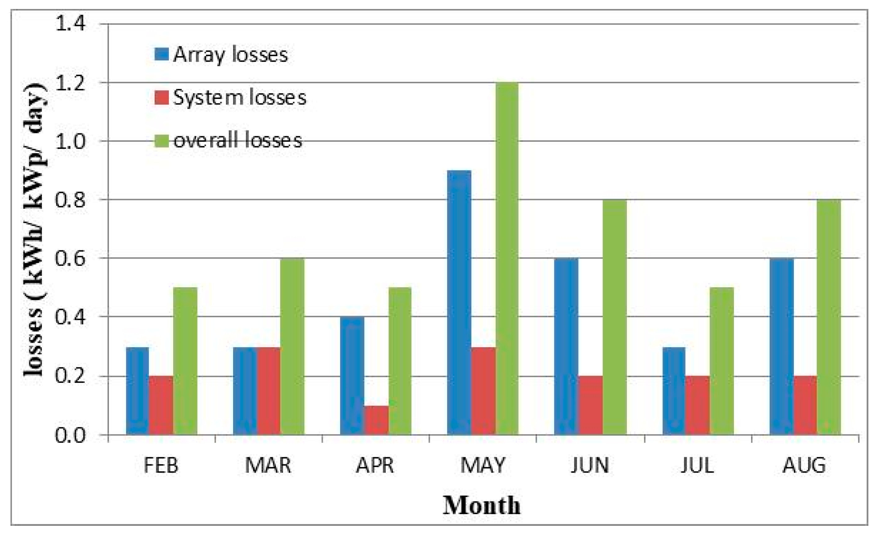
The modules capture losses (Lm) which are the difference between the reference yield (YR) and the array performance (Ym), it represents the losses due to the operation of the modules that demonstrate the inability of the system to fully utilize the available irradiance [46]. They are obtained by Equation (4):
L m = Y R Y m ( kWh kW p )
The inverter losses (LI) due to the conversion from DC power output to AC power in PV solar panels. They are given by Equation (5):
L I = Y m Y F ( kWh kW p )
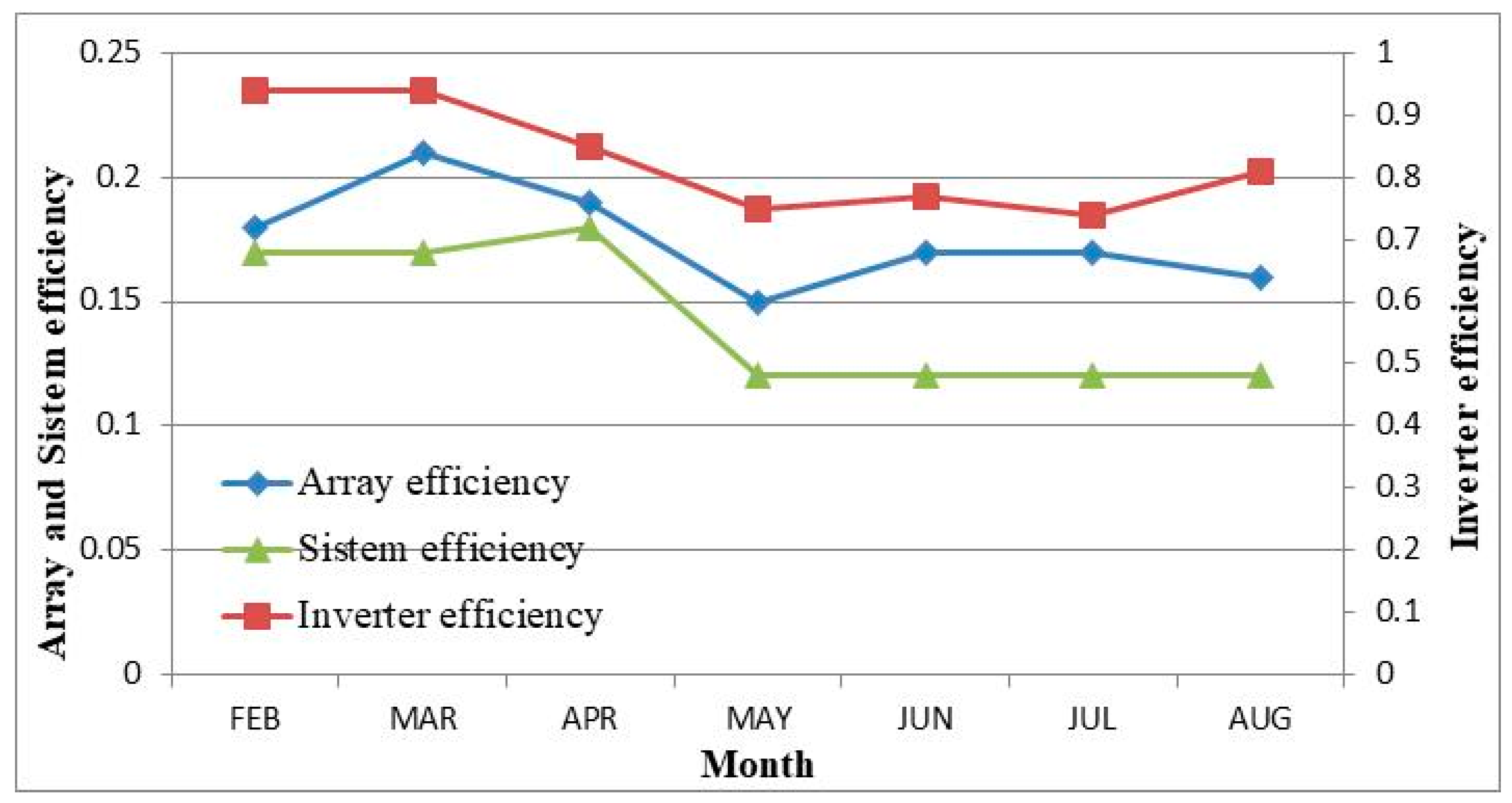
The efficiency of a PV system can be grouped into three categories: the photovoltaic module efficiency, system efficiency and inverter efficiency. The photovoltaic module efficiency ( η P V ), is the relationship between the daily output power (ED) and the total daily irradiation product in the (GT) plane and the area of the photovoltaic array (Am) [46]. PV module efficiency is calculated by the Equation (6):
η P V = 100   ×   E D G T   ×   A m ( % )
The system efficiency ( η S ) represents the performance of the entire PV system installed and is calculated by the Equation (7) and the inverter efficiency ( η I ) by the Equation (8):
η S = 100   ×   E A G T   ×   A m ( % )
η I = 100   ×   E A E D   ( % )

2.3. Power Quality

Power quality is needed to check the physical properties of the systems, such as amplitude, frequency, waveform, current and voltage. The most important standards for Colombia are: Electromagnetic Compatibility (IEC 61000-4-7, 2002), Recommended Practices and Requirements for Harmonic Control in Electrical Power Systems (IEEE 519, 1992), Energy Quality (NTC-5001, 2008)), Nominal Voltage and Frequency of Electric Power Systems in Service Networks (NTC-1340, 1998), Regulatory Commission for Energy and Gas (CREG 070,1998; 096, 2000; 084, 2002; 0024, 2005), and finally, the Technical Regulation on electrical installations (RETIE).

3. Methodology

In the energy quality studies, the proposed methodology follows the basic steps presented by some authors [47] and the Colombian Technical Standard NTC 5001, the measurement period should be one week with a period aggregation of 10 min for the long-term or permanent perturbations, and 10 s for slow and rapid disturbances.
The measurements were recorded at two different points: First, the solar irradiance, wind speed, ambient temperature and panel temperature were recorded as seen in Figure 3. Second, the voltage and current AC/DC were recorded at the point of common coupling (Figure 4).

4. Equipment

The most important instruments for the measurement of variables of interest in the location are described as follows.
  • Turbine Anemometer (model ETAI-30, Erasmus, Ibagué, Colombia). Records the room temperature in the range of −10 °C to 60 °C, resolution of 0.1 °C and accuracy of ±2 °C; Also, the wind speed in the range of 0.40 to 30.0 m/s, with resolution of 0.01 m/s and accuracy of ± (3% + 0.2 m/s).
  • Digital clamp multimeter (Erasmus model EPD-1000). Records the AC/DC voltage and current in the range of 0.01to 1000 A and 0 to 600 V, resolution of 0.01 A and 0.01 V, accuracy of ±5% for both, AC/DC voltage and current.
  • Solar energy meter (Erasmus model ES-2000). Records the solar irradiation in the range of 0 to 1999 W/m2, resolution of 1 W/m2 and accuracy of ±5%.
  • Infrared Pyrometer (model 94920/EM520, All-sun, Ibagué, Colombia). Records the temperature without surface contact in the range of −20 °C to 520 °C, resolution of 0.1 °C and accuracy of ±2%.
  • Power analyzer (model PW 3360-21, HIOKI, Ibagué, Colombia). Effective Range: Voltage: 90 V to 780 V; Peak: ±1.400 V; Current: 5% to 110% of range; Power: 5% to 110% of range; Frequency: 45 Hz to 66 Hz.

5. Results and Discussion

The variables described above were measured to calculate the energy production, the system efficiencies, losses, as well as calculation of evaluation parameters and power quality.

5.1. System Efficiency

Figure 5 shows the maximum energy output of the photovoltaic system in March 2016 with 72.65% (850 kWh) of the total installed capacity (1170 kWh). This percentage is similar to those found by [48,49], which recorded 70%; Moreover, it is very close to the values between 80% and 100% given in other references [50].
The lowest production was obtained in June 2016 with 49.42% (578.21 kWh), due to the high cloudiness and the rainy season. In a 7-month period, 4707.14 kWh was produced with a monthly average of 672.45 kWh. Considering that the average is kept for a year, energy produced will be 8069.4 kWh.
The final energy produced during the period divided by the nominal power of the system is 1034.5 kWh/kWp, a value that is lower than that found in cities and countries like Tiruchirappalli (India), 1600 kWh/kWp; Málaga (Spain), 1339 kWh/kWp; Crete (Greece) 1336.4 kWh/kWp; Calabria (Italy) 1230 kWh/kWp; Israel 1840 kWh/kWh and India 1372 kWh/kWh, and higher than those recorded in countries such as The Netherlands 700 kWh/kWh; Germany 730 kWh/kWp and Switzerland 790 kWh/kWp [33].
The lowest solar irradiation value was registered during February and the highest was in May. In the other hand, ambient temperature ranged from 25.1 °C in June to 35.99 °C in May, showing an upward trend and wind speed ranged from 0.3 m/s to 1.1 m/s. Solar radiation presents a maximum value of 820 W/m2/month at 11:00 and a minimum of 200 W/m2/month at 16:00 h, remaining constant between 11:00 and 14:00 h.
In contrast, the equation that correlates the electrical energy output (EA) with the solar radiation (G) is EA = 3.769G–613.8 with a correlation coefficient of 0.929. Figure 6 shows that the output power (EA) has a linear relationship with solar radiation. The importance of an equation like this is that it makes possible to evaluate the generation of energy using photovoltaic power systems, only by identifying the solar radiation.
The error rate obtained with the equation is, within the experimental uncertainty, higher than the values presented by [29] (5%), and lower than those reported by [32] (15%). The differences could be due to the specific characteristics of each photovoltaic system, the manufacturers and the climatic conditions.
Subsequently, in Figure 7, it is observed that the lowest values of the monthly reference mean (YR), Module (Ym) and final yields (YF) coincide with the rainy season and are 3.0 kWh/kWp/day, 2.8 kWh/kWp/day and 2.6 kWh/kWp/day, respectively, during the months of June and July 2016. The highest reference performance values of 3.9 kWh/kWp/day were recorded in May 2016, the yields of the modules and final were 3.5 kWh/kWp/day and 3.2 kWh/kWp/day for the March 2016, respectively.
Monthly averages were also obtained during the measurement period of YR, Ym and YF of 3.4 kWh/kWp/day, 3.2 kWh/kWp/day and 3.0 kWh/kWp/day, respectively. Due to the energy losses that occur in the DC/AC conversion in the inverter, the differences presented in the YF and Ym values are justified, since the room temperature for Ibagué oscillates between 16 and 29 °C and some authors [51] have observed that for every 12 °C increase in ambient temperature the efficiency of the inverter drops approximately 1%.
The average final yield of the present study was 3.0 kWh/kWp/day, being lower than that found in cities such as Nicosia (Cyprus), where the average final yield was 4.3 kWh/kWp/day, Sawda (Kuwait) with a final yield of 4.5 kWh/kWp/ day [29] and Ceará (Brazil) with a final yield of 4.6 kWh/kWp/day [52]. The difference is that Ibagué has a predominantly dry tropical climate and in the cities of Nicosia, Sawda and Ceará the climate is semi-arid.
The largest losses of the modules (Lm) occurred in May with a value of 0.9 kWh/kWp/day and the lowest in March of 0.3 kWh/kWp/day, Figure 8, values corresponding to 23.08% and 9% of the reference yields of the respective months. The values found are similar to those reported in the literature for cities such as Rajkot (India), where capture losses were 22.27% and 3.79% of the respective reference yields [53]; the number in Singapore was 22.66% and 17.06% [46] and Ceará (Brazil) with 22.5% and 2.3% [52], respectively.
In addition, the losses in the system varied from 0.30 kWh/kWp/day in March to 0.10 kWh/kWp/day in April, corresponding to 9.0% and 3.0% of the respective reference yields. The values found are higher than those reported in cities such as Singapore of 5.55% and 5.06% [46] and Fortaleza (Brazil), with 5.7% and 4.2% [52] and lower than in Mauritania of 26.3% and 3.55% [44], Lesotho with 18.57% and 10.34% [33] and Ireland with 22.23% and 2.89% [54].
On the other hand, the maximum total loss ocurred in May and the minimum in April with values of 1.1 kWh/kWp/day and 0.4 kWh/kWp/day, respectively. These values correspond to 29% and 12% of the respective reference yields. The values differed very little from those reported by [52] of 27.1% and 6%. The average annual loss of the inverter and total losses was 0.5 kWh/kWp/day, 0.20 kWh/kWp/day and 0.7 kWh/kWp/day, respectively. These values are lower than those reported from 0.71 kWh/kWp/day, 0.27 kWh/kWp/day and 1.05 kWh/kWp/day [52].
To continue, in Figure 9, the highest efficiency values of the modules, the system and the inverter were obtained during March and April with values of 21%, 18% and 94%, respectively. The lowest in May and June with values of 15%, 12% and 74%, respectively. The average monthly efficiency of the modules, the system and the investor during the registration period are 17.6%, 14.3% and 82.8%, respectively. The maximum values are found early in the morning and the minimum values at the end of the day.
Besides, the highest efficiency occurred in March with an average value of 21%, and the lowest in May with 15% Figure 10. These results are similar to the 15.9% obtained in the laboratory under controlled conditions, as well as the range of 15–20%, found in the literature [55]. During the first three months of operation the efficiency is high, but from this point it decreases due to the effects of soiling caused by contamination. This coincides with the case of a similar system presented by [56] and also with the time recommended by the manufacturer to do the maintenance in the solar panels.
Lastly, the efficiency of photovoltaic modules is not affected in the irradiation interval between 400 and 1000 W/m2, being consistent with what is expressed in [55]. The average efficiency of the inverter was in the range of 75–94% for the different values of irradiation. These results are comparable with the efficiency reported by the manufacturer of 96.9%; also, they are similar to those found in studies conducted in Europe and the United States with mean values of 88% for Fronius inverters [57].

5.2. Power Quality at the Point of Common Coupling

When comparing the measurements of active power before and after the installation of the photovoltaic solar system, Figure 10 and Figure 11 showed no significant difference, during the academic term there was a maximum consumption of 190 kWh/day and a minimum of 30 kWh/day. During Sunday, a decrease in consumption of 8 kWh/day from 10:00 a.m. to 3:00 p.m., coinciding with the period of operation of the photovoltaic system and the absence of academic activity at the Universidad de Ibagué. Therefore, it is confirmed that the photovoltaic system contributes to the active energy consumption, being visible in periods of low demand. The reactive power consumption increased by 7% in relation to the maximum value recorded and 40% in relation to the minimum obtained.
Regarding the variation of the steady-state voltage, before and after the installation of the photovoltaic system, there is no negative impact on the lines (U1, U2 and U3), according to the guidelines of standards NTC 5001, IEC 038 and EM 50160, there were no overvoltages or undervoltages. Figure 12 and Figure 13 represent the percentage of the recorded voltage values compared to the declared RMS voltage values (120 V).
The maximum percentage obtained was of 102.87% and the minimum of 94.08% with respect to the standard value of 100% proposed by the NTC 5001. The value of the voltage after installing the experimental system is more stable because the inverter only injects energy when it is in synchronism with the network (Figure 6), the value of the voltage registered an increase of 7.88%, 5.87% and 6.27% in the lines U3, U2 and U1, after installing the experimental system. The values found are similar to those reported by [58,59], who found very small increases, that in some cases reached 2%.
The voltage unbalance is maintained within the ranges established by NTC 5001 before and after the connection of the photovoltaic system (Table 3). When installing the experimental system the value of the average voltage is very close to the value of the registered voltage, that is to say, the standard deviation is smaller and the value of the voltage is more stable, this causes the unbalance factor to be improved. However, it registers an increase of 3.5% and 70% with respect to the maximum and minimum values, respectively. These results go along with the suggestions made by some authors [60] that show the possibility of an increase in the voltage unbalance with the installation of photovoltaic systems in low voltage grids.
Short and long term flicker measurements before and after installation of the photovoltaic network is within the range established by NTC 5001 and EM 50160 (Table 4 and Table 5). The maximum and minimum values obtained during short-duration flicker measurements were 0.35 and 0.10 p.u., respectively. The long duration flicker recorded a maximum value of 0.20 p.u. and a minimum of 0.09 p.u. The values obtained from the flicker variation that short and long duration are below those reported in the literature [61], who found a value of 0.38 p.u. in short duration flicker measurements in a photovoltaic system connected to the low voltage network 7.2 kWp. Similar studies performed by [62] recorded long-duration flicker values of 0.36 p.u.
The values of total voltage harmonics (THD) that were recorded before and after the operation of the photovoltaic system are lower than the 5.0% value established by NTC 5001 (Table 6). The maximum value obtained was 3.75% and the minimum of 1.70%. However, in all the lines, it is possible to identify an increase of 7% for line U1, 0.8% in U2 and 3%, in line U3. Increases are produced by leakage currents that increase harmonics and electromagnetic emissions in the existing power structure [62]. When the inverter operates with a relative power greater than 20% and the voltage is sinusoidal, the current injected into the network by the inverter is also sinusoidal with low harmonic content; therefore, a high quality inverter can have harmonics content levels limited to those established by technical standards in the highest possible power range. However, when the relative power is less than 20%, depending on the manufacturer, the inverters can present currents with harmonic distortion levels higher than the values established by the technical standards. The total harmonic distortion tends to increase when the load level of the inverter decreases, regardless of the impedance of the network. Is possible to find situations where the reactive electrical charges at the connection point interfere with the harmonic current. Another reference also found an increase between 0.7% and 2.5% in an 8 kWp system [63].
The total current harmonics (TDDI) recorded and compared to the NTC 5001 are outside the established range (Table 7), with a maximum value of 17.80% and minimum of 0.80%. The values recorded before and after the implementation of the photovoltaic system do not present significant differences for the lines U2 and U3, in line U1, an increase 22% was obtained. This increase is consistent with that reported by some authors [64] and similar to that reported by [63], who found values between 2 and 38% when studying an experimental network of 8 kWp.
The power factor was not affected by the operation of the photovoltaic system (Table 8), and a maximum value of 0.98 and a minimum of 0.85 were obtained, in compliance with the guidelines of NTC 5001. These values are in agreement with [65,66,67] which state that the power factor must be greater than 0.85 if the recording at the output of the photovoltaic system is greater than 10% of the capacity. The power factor of the inverter is a function of the load level and increases proportionally to the relative power, approaching 100% when it is working with the nominal output power. For inverters that operate above 30% of the rated power, the power factor is greater than 90% and for values below 30%, the power factor is lower.
The total active and reactive power were increased by 58% and 42% after the photovoltaic system started operating (Table 9 and Table 10). The registered maximum value of active and reactive power was 33.88 kW and 9.5 kW, respectively. The reduction of the power during the faults on the network is a major problem for DG power plants. The deeper the network failure, the higher the reactive power requirements of the network operators [68]. In extreme cases, 100% of the reactive current is required. However, in gaps produced far from the connection point, both active and reactive power must be injected to feed and support the network simultaneously. Excess production must be eliminated from the system to avoid overvoltage and inverter trip, if the network voltage drops, the inverter injects capacitive reactive current to increase it and if it increases, the inverter injects inductive current to decrease it, these voltage variations of the network change the active and reactive power after the installation of the PV photovoltaic system.
The maximum and minimum temperatures obtained at the common connection point before the photovoltaic system came into operation were 34.3 °C and 31.4 °C, respectively (Figure 14). Once the system came into operation, the maximum and minimum temperatures recorded were 36.9 °C and 33.7 °C, respectively (Table 11). Therefore, the increase at the common point of connection of the temperature is 7.5%. This increase is within the requirements established by the NTC 2050 and the BWG.

6. Conclusions

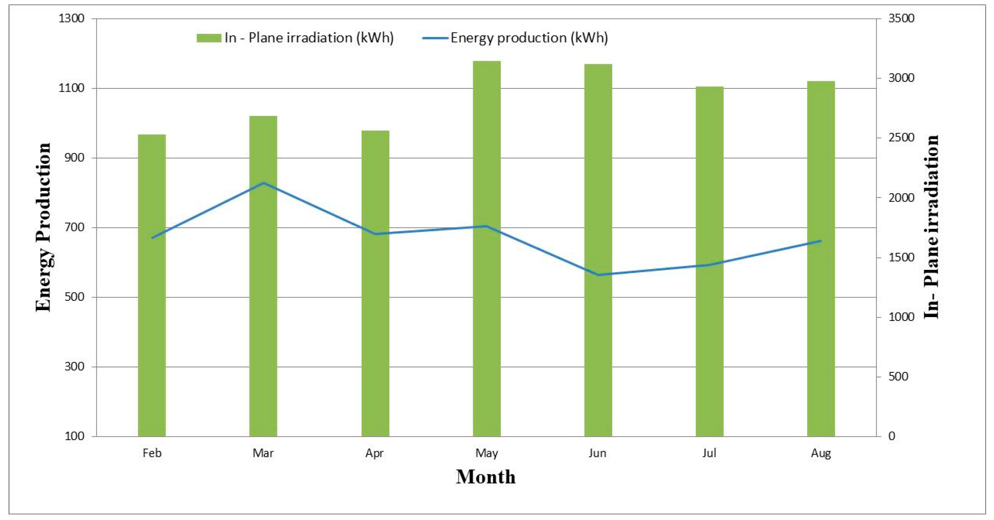
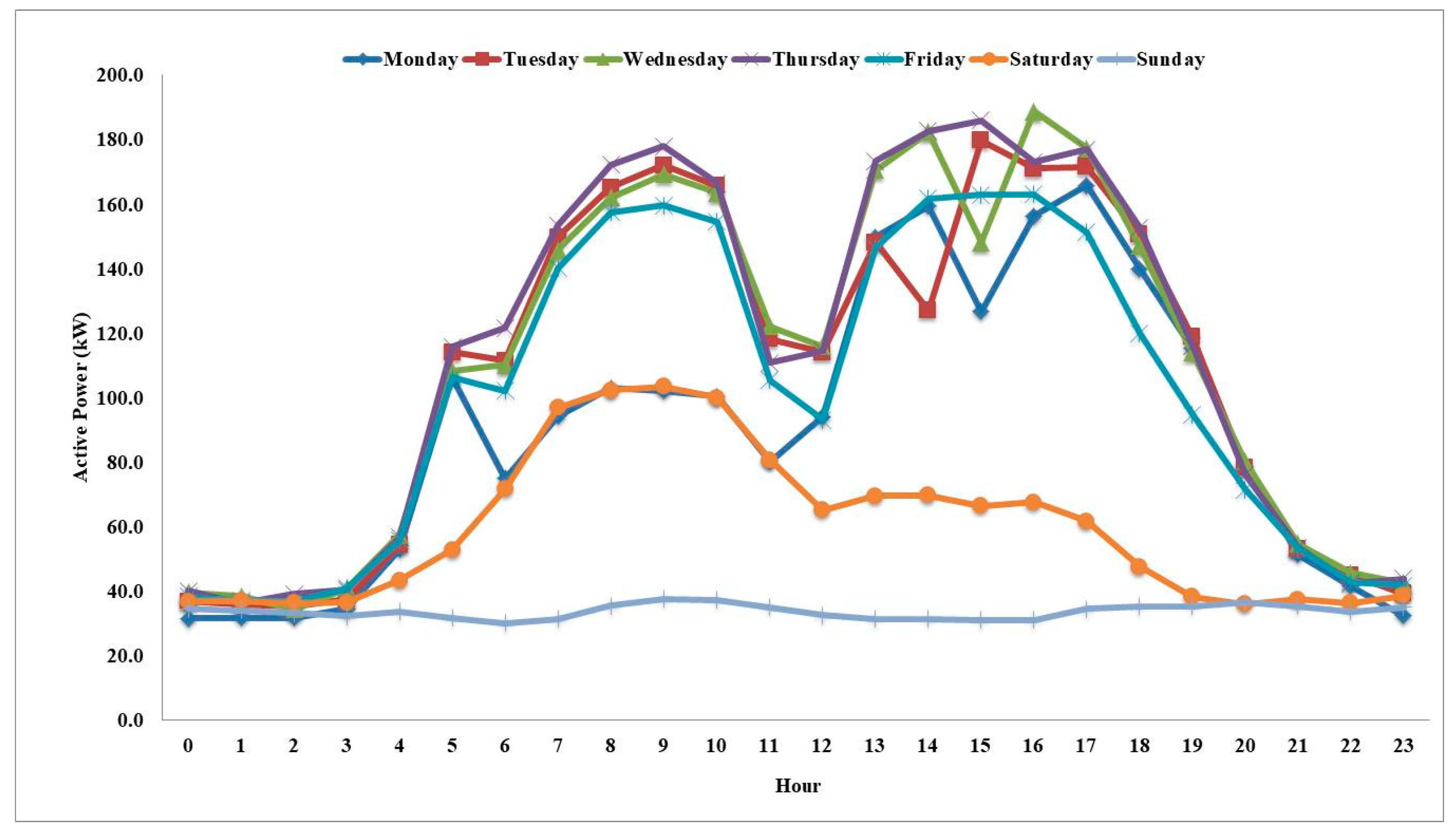
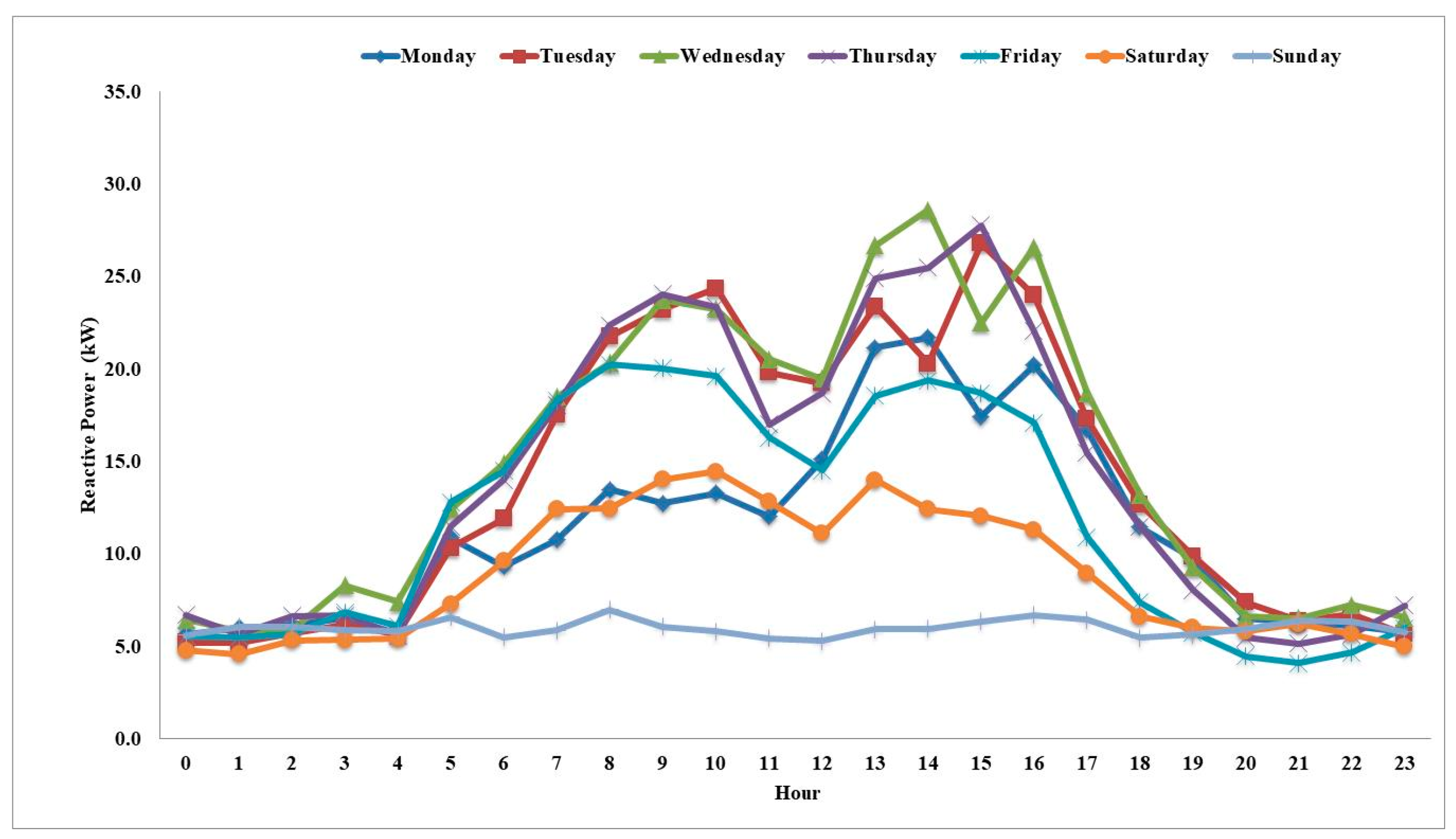
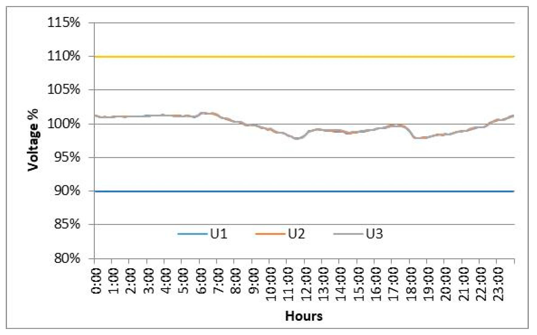
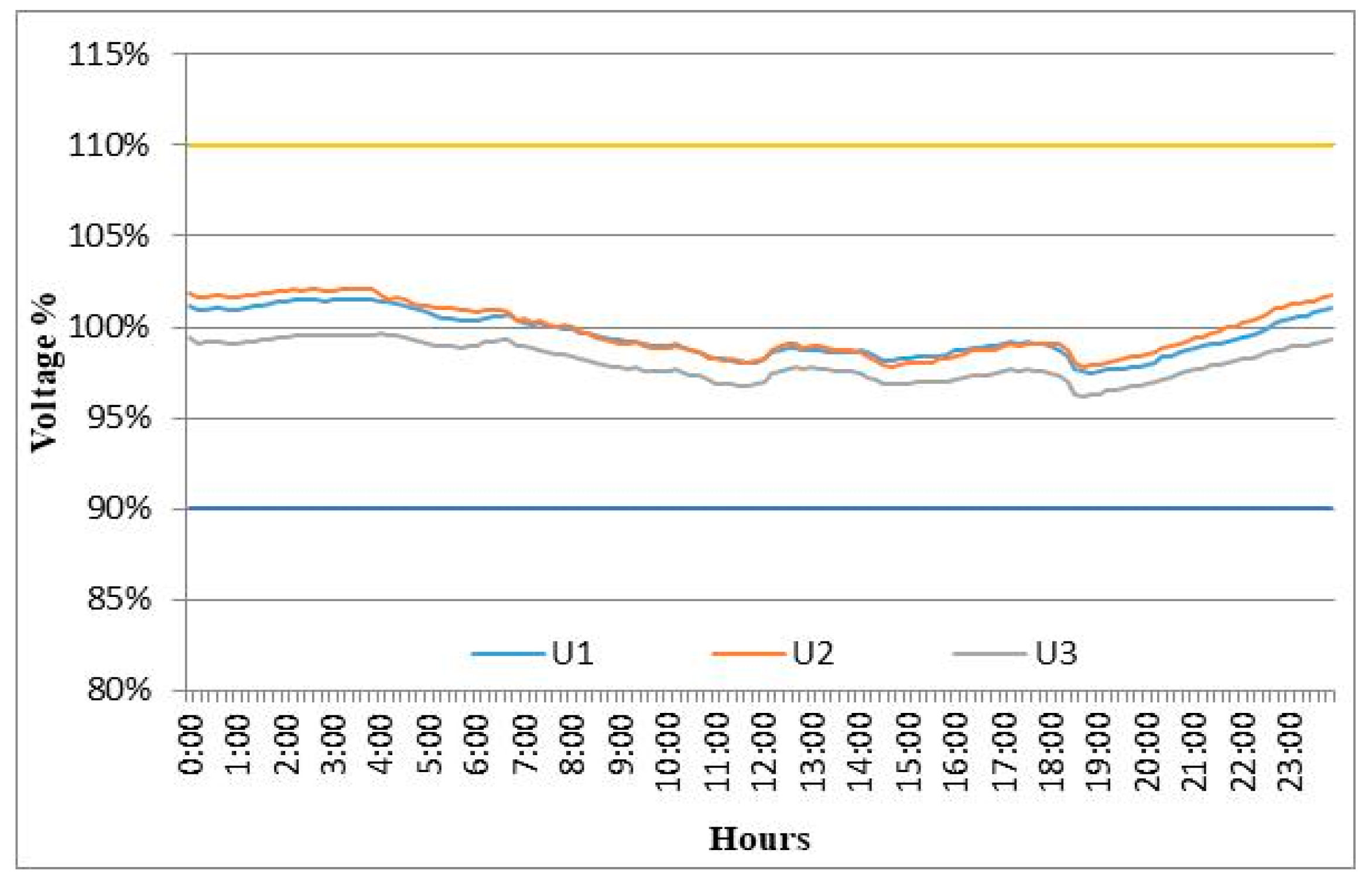
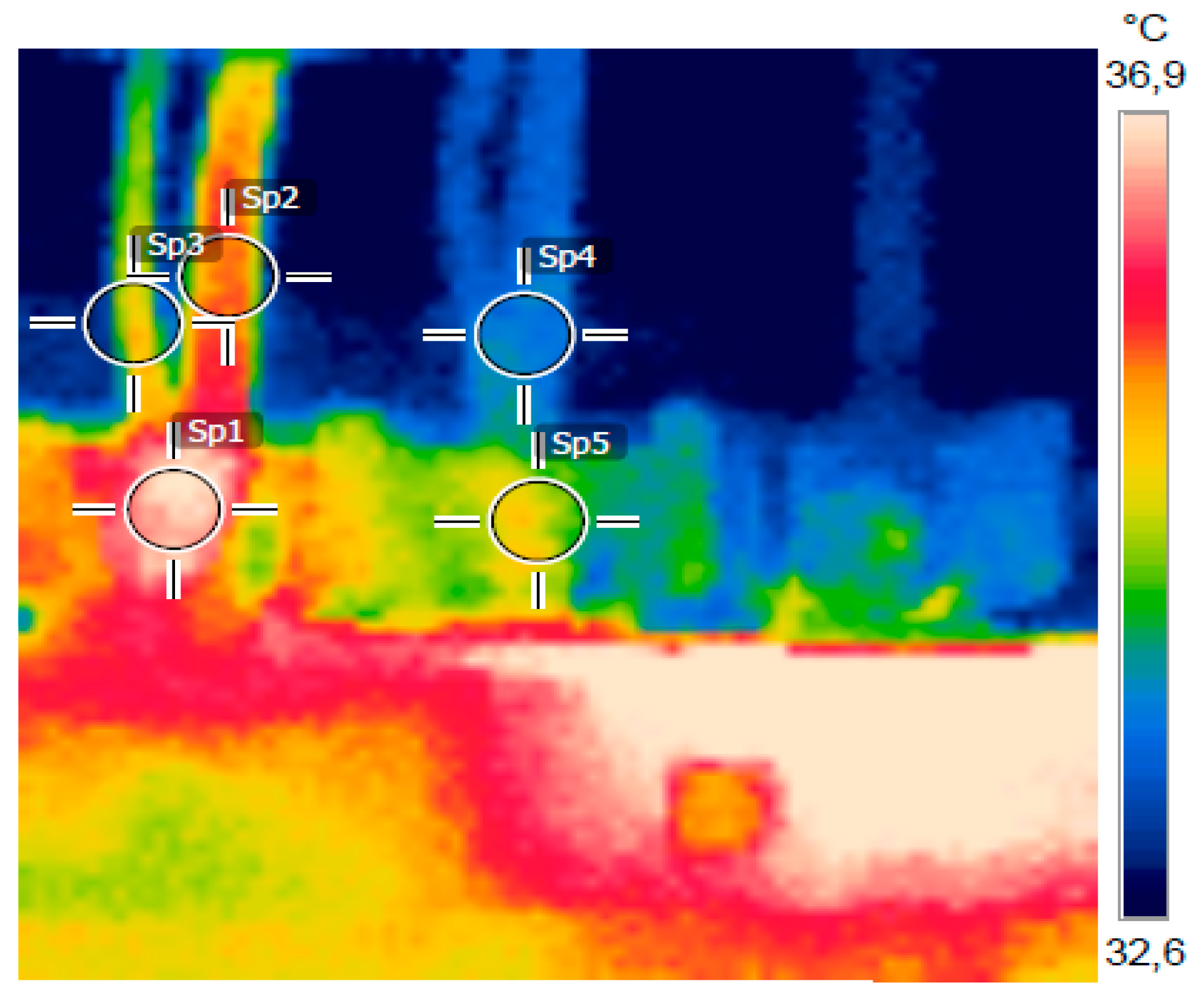
A study of a photovoltaic system of 7.8 kWp connected to the low voltage electrical grid belonging to the Universidad de Ibagué Colombia, from February to August 2016, determining its performance parameters and the energy quality at the common point of connection, is reported. The total energy produced was 8069.4 kWh and the final energy produced during the period divided by the nominal power of the system is 1034.5 kWh/kWh. The benchmark performance, module performance and final performance values ranged from a minimum to a maximum of 3.0–3.9 kWh/kWp/day; 2.8–3.5 kWh/kWp/day and 2.6–3.2 kWh/kWp/day, respectively. The average annual losses in the module, inverter and total losses were 0.5 kWh/kWp/day, 0.20 kWh/kWp/day and 0.7 kWh/kWp/day. The average monthly efficiency of the modules, the system and the investor during the registration period are 17.6%, 14.3% and 82.8%, respectively. Reactive power consumption increased between 7% and 40%. The voltage unbalance registers an increase of 3.5% and 70% with respect to the maximum and minimum values, respectively. The maximum and minimum value obtained during short and long duration flicker measurements was 0.35 p.u., 0.20 p.u. and 0.10 p.u., 0.09 p.u., respectively. The values of total voltage harmonics (THD) increased by 7% for the U1 line, 0.8% for U2 and 3% for the U3 line, and TDDI current harmonics recorded a 22% increase. The total active and reactive power were increased by 58% and 42% after the photovoltaic system started operating and the temperature at the common point of connection increased by 7%. The results show the importance of this type of study, because the vast majority of low voltage grids in Colombia are old, they are saturated and any disturbance can cause serious damage to the connected electrical devices. It is important to know the impact on the power quality caused by the installation of photovoltaic systems to the low voltage grid, in order to define the requirements of the network, the type of communication between the photovoltaic system and the operator of the low voltage grid, the necessary protection system, among others.

Author Contributions

A.V.G. and T.M.d.S. conducted the experiments; A.V.G., T.M.d.S. and P.M.S. analyzed the data; A.V.G. and D.F.A.S. edited and improved the manuscript.

Acknowledgments

This work was supported by the Universidad de Ibagué and Universidade Estadual Paulista (UNESP) Câmpus Guaratinguetá under Project 15-333-INT.

Conflicts of Interest

The authors declare no conflict of interest.

References

  1. Jacovides, C.P.; Tymvios, F.S.; Assimakopulous, V.D.; Kaltsounides, N.A. Comparative study of various correlations in estimating hourly diffuse fraction of global solar radiation. Renew. Energy 2006, 31, 2492–2504. [Google Scholar] [CrossRef]
  2. Yang, D.; Yin, H. Energy conversion efficiency of a novel hybrid solar system for photovoltaic, thermoelectric, and heat utilization. IEEE Trans. Energy Convers. 2011, 26, 662–670. [Google Scholar] [CrossRef]
  3. Phuangpornpitak, N.; Kumar, S. User acceptance of diesel/PV hybrid system in an island community. Renew. Energy 2011, 36, 125–131. [Google Scholar] [CrossRef]
  4. Yilmaz, S.; Ozcalik, H.; Kesler, S.; Dincer, F.; Yelmen, B. The analysis of different PV power systems for the determination of optimal PV panels and system installation—A case study in Kahramanmaras, Turkey. Renew. Sustain. Energy Rev. 2015, 52, 1015–1024. [Google Scholar] [CrossRef]
  5. Chouder, A.; Silvestre, S. Automatic supervision and fault detection of PV systems based on power losses analysis. Energy Convers. Manag. 2010, 51, 1929–1937. [Google Scholar] [CrossRef]
  6. Energy Information Administration. Annual Energy Review 2008. 26 June 2009. Available online: https://www.eia.gov/totalenergy/data/annual/archive/038408.pdf (accessed on 15 May 2015).
  7. REN21. September 2011. Available online: http://www.ren21.net/Portals/0/documents/Resources/GSR2011_FINAL.pdf (accessed on 15 May 2015).
  8. Markvart, T. Solar Electricity; Wiley: Chichester, UK; New York, NY, USA, 2000. [Google Scholar]
  9. Caamaño-Martin, E. Edificios Fotovoltaicos Conectados a La Red Electrica: Caracterizacion y Analisis. Ph.D Thesis, E.T.S.I. Telecomunicación (UPM), Madrid, Spain, 1998. [Google Scholar]
  10. Bagarella, G.; Lazzarin, R.; Noto, M. Annual simulation energy and economic analysis of hybrid heat pump systems for residential buildings. Appl. Therm. Eng. 2016, 99, 485–494. [Google Scholar] [CrossRef]
  11. Pärisch, P.; Mercker, O.; Warmuth, J.; Tepe, R.; Bertram, E.; Rockendor, G. Investigations and model validation of a ground-coupled heat pump for the combination with solar collectors. Appl. Therm. Eng. 2014, 62, 375–381. [Google Scholar] [CrossRef]
  12. Hoseini, M.; Rahdar, A.; Emamzadeh, A. A comparative study on PCM and ice thermal energy storage tank for air-conditioning systems in office buildings. Appl. Therm. Eng. 2016, 96, 391–399. [Google Scholar] [CrossRef]
  13. Mayer, B.; Killian, M.; Kozek, M. Management of hybrid energy supply systems in buildings using mixed-integer model predective control. Energy Convers. Manag. 2015, 98, 470–483. [Google Scholar] [CrossRef]
  14. Shihabudheen, M.; Arun, P. Performance evaluation of a hybrid photovoltaic-thermal water heating system. Int. J. Green Energy 2015, 9, 969–986. [Google Scholar] [CrossRef]
  15. Zafar, S.; Dincer, I. Thermodynamic analysis of a combined Pv/T-fuel cell system for power, heat, fresh water and hydrogen production. Int. J. Hydrogen Energy 2014, 39, 9962–9972. [Google Scholar] [CrossRef]
  16. Herrando, M.; Markides, C.; Hellgardt, K. A UK-based assessment of hybrid PV and solar-thermal systems for domestic heating and power system performance. Appl. Energy 2014, 122, 288–309. [Google Scholar] [CrossRef]
  17. Shaari, S.; Omar, A.M.; Haris, A.H.; Sulaiman, S.I. Solar Photovoltaic Power: Designing Grid-Connected Systems; Kementerian Tenaga, Teknologi Hijau dan Air: Putrajaya, Malaysia, 2010. [Google Scholar]
  18. Alonso-Abella, M. A model for energy production estimation of PV grid connected systems based on energetic losses and experimental data on site diagnosis. In Proceedings of the 19th European Photovoltaic Solar Energy Conference, Paris, France, 7–11 June 2004; pp. 2447–2450. [Google Scholar]
  19. Gabler, H.; Wiemken, E. How much energy will a specific PV system produce? In Proceedings of the Actas del XIII Congreso Europeo de Energia Solar Fotovoltaica, Niza, France, 23–27 October 1995. [Google Scholar]
  20. Ransome, S.J.; Wohlgemuth, J.H. kWh/kWp dependency on PV technology and balance of systems performance. In Proceedings of the Conference Record of the Twenty-Ninth IEEE Photovoltaic Specialists Conference, New Orleans, LA, USA, 19–24 May 2002. [Google Scholar]
  21. Kroposki, B.; Emery, K.; Myers, D.; Mrig, L. A comparison of photovoltaic module performance evaluation methodologies for energy ratings. In Proceedings of the 1994 IEEE 1st World Conference on Photovoltaic Energy Conversion—WCPEC (A Joint Conference of PVSC, PVSEC and PSEC), Waikoloa, HI, USA, 5–9 December 1994. [Google Scholar] [Green Version]
  22. Turcotte, D.; Ross, M.; Sheriff, F. Photovoltaic hybrid system sizing and simulation tools: Status and Needs. In Proceedings of the PV Horizon: Workshop on Photovoltaic Hybrid Systems, Montreal, QC, Canada, 10 September 2001. [Google Scholar]
  23. King, D.L.; Boison, W.E.; Kratochvil, J.A. Energy-Based performance modeling for photovoltaic systems. In Proceedings of the National Center for Photovoltaics and Solar Program Review Meeting, Denver, CO, USA, 24–26 March 2003. [Google Scholar]
  24. Abete, A.; Napoli, R.; Spertino, F. A simulation procedure to predict the monthly energy supplied by grid-connected Pv systems. In Proceedings of the 3rd World Conference on Photovoltaic Energy Conversion, Osaka, Japan, 11–18 May 2003. [Google Scholar]
  25. Šúri, M.; Huld, T.A.; Dunlop, E.D. PV-GIS: A web-based solar radiation database for the calculation of PV potential in Europe. Int. J. Sustain. Energy 2005, 24, 55–67. [Google Scholar] [CrossRef]
  26. Carneiro, J.A.O. Dimensionamento de Sistemas Fotovoltaicos. Ph.D. Thesis, Instituto Politécnico de Bragança, Escola Superior de Tecnologia e de Gestão, Guimaraes, Portugal, 2009. [Google Scholar]
  27. Hernández Mora, J.A. Metodología Para El Análisis Técnico De La Masificación De Sistemas Fotovoltaicos Como Opción De Generación Distribuida En Redes De Baja Tensión; Universidad Nacional de Colombia: Bogota, Colombia, 2012. [Google Scholar]
  28. Patiño Abella, J.S.; Tello Reyes, J.S.; Hernandez Mora, J.A. Diseño e implementación de un sistema fotovoltaico híbrido y desarrollo de su regulador de carga aplicando instrumentación virtual. Elementos 2013. [Google Scholar] [CrossRef]
  29. Adaramola, M.S.; Vagnes, E.E. Preliminary assessment of a small-scale rooftop PV-grid tied in Norwegian climatic conditions. Energy Convers. Manag. 2015, 90, 458–465. [Google Scholar] [CrossRef]
  30. Micheli, D.; Alessandrini, S.; Radu, R.; Casula, I. Analysis of the outdoor performance and efficiency of two grid connected photovoltaic systems in northern Italy. Energy Convers. Manag. 2014, 80, 436–445. [Google Scholar] [CrossRef]
  31. Diez-Mediavilla, M.; Alonso-Tristan, C.; Rodriguez-Amigo, M.; Garcia-Calderon, T.; Dieste-Velasco, M. Performance analysis of PV plants: Optimization for improving profitability. Energy Convers. Manag. 2012, 54, 17–23. [Google Scholar] [CrossRef] [Green Version]
  32. Ayompe, L.; Duffy, A.; McCormack, S.; Conlon, M. Measured performance of a 1.72 kW rooftop grid connected photovoltaic system in Ireland. Energy Convers. Manag. 2011, 52, 816–825. [Google Scholar] [CrossRef]
  33. Mpholo, M.; Nchaba, T.; Monese, M. Yield and performance analysis of the first grid-connected solar farm at Moshoeshoe I International Airport, Lesotho. Renew. Energy 2015, 81, 845–852. [Google Scholar] [CrossRef] [Green Version]
  34. Kumar, K.A.; Sundareswaran, K.; Venkateswaran, P. Performance study on a grid connected 20 kWp solar photovoltaic installation in an industry in Tiruchirappalli (India). Energy Sustain. Dev. 2014, 23, 294–304. [Google Scholar] [CrossRef]
  35. Padmavathi, K.; Daniel, S.A. Performance analysis of a 3 MWp grid connected solar photovoltaic power plant in India. Energy Sustain. Dev. 2013, 17, 615–625. [Google Scholar] [CrossRef]
  36. Marnay, C. Micro-Grids and Heterogeneous Security, Quality, Reliability and Availability. In Proceedings of the Power Conversion Conference, Nagoya, Japan, 2–5 April 2007. [Google Scholar]
  37. Li, Y.; Vilathgamuwa, D.; Loh, P. A Grid-Interfacing Power Quality Enchanced Operation of a Three-Wire Micro-Grid Applications. IEEE Trans. Power Electron. 2006, 21, 1021–1031. [Google Scholar] [CrossRef]
  38. Majumder, R.; Ghosh, A.; Ledwich, G.; Zare, F. Load Sharing and Power Quality Enchanced Operation of a Distributed Micro-Grid. IET Rev. Power Gener. 2009, 3, 109–119. [Google Scholar] [CrossRef] [Green Version]
  39. Shahnia, F.; Majumder, R.; Ghosh, A. Operation and Control of a Hybrid Micro-Grid Containing Unbalanced and Nonlinear Loads. Electr. Power Syst. Res. 2010, 80, 954–965. [Google Scholar] [CrossRef] [Green Version]
  40. Papadimitriou, C.; Vovos, N. Transient Response Improvement of Microgrids Exploiting the Inertia of a Doubly-Fed Induction Generator (DFIG). Energies 2010, 3, 1049–1066. [Google Scholar] [CrossRef] [Green Version]
  41. Zamani, M.; Yazdani, A.; Sidhu, T. A Control Strategy for Enhanced Operation of Inverter-Based Micro-Grids Under Transient Distrubances and Network Faults. IEEE Trans. Power Deliv. 2012, 27, 1737–1747. [Google Scholar] [CrossRef]
  42. Dávi, G.A.; Caamaño-Martin, E.; Rüther, R.; Solano, J. Energy performance evaluation of a net plus-energy residential building with grid-connected photovoltaic system in Brazil. Energy Build. 2016, 120, 19–29. [Google Scholar] [CrossRef]
  43. Adaramola, M.S. Techno-economic analysis of a 2.1 kW rooftop photovoltaic-grid-tied system based on actual performance. Energy Convers. Manag. 2015, 101, 85–93. [Google Scholar] [CrossRef]
  44. Sidi, C.E.; Ndiaye, M.L.; El Bah, M.; Mbodji, A.; Ndiaye, A.; Ndiaye, P.A. Performance analysis of the first large-scale (15 MWp) grid-connected photovoltaic plant in Mauritania. Energy Convers. Manag. 2016, 119, 411–421. [Google Scholar] [CrossRef]
  45. Sharma, V.; Chandel, S. Performance analysis of a 190 kWp grid interactive solar photovoltaic power plant in India. Energy 2013, 55, 476–485. [Google Scholar] [CrossRef]
  46. Wittkopf, S.; Valliappan, S.; Liu, L.; Ang, K.S.; Cheng, S.C. Analytical performance monitoring of a 142.5 kWp grid-connected rooftop BIPV system in Singapore. Renew. Energy 2012, 47, 9–20. [Google Scholar] [CrossRef]
  47. Santoso, S.; McGranaghan, M.F.; Wayne Beaty, H. Electrical Power Systems Quality, 3rd ed.; McGraw-Hill Education: Berkshire, UK, 2012. [Google Scholar]
  48. Burger, B.; Rüther, R. Inverter sizing of grid-connected photovoltaic systems in the light of local solar resource distribution characteristics and temperature. Solar Energy 2006, 80, 32–45. [Google Scholar] [CrossRef]
  49. Macedo, W.; Zilles, R. Operational results of grid-connected photovoltaic system with different inverter’s sizing factors (ISF). Prog. Photovolt. Res. Appl. 2007, 15, 337–352. [Google Scholar] [CrossRef]
  50. Islam, S.; Woyte, A.; Belmans, R.; Nijs, J. Undersizing inverters for grid connection—What is the optimum? In Proceedings of the PV in Europe, Rome, Italy, 7–11 October 2002. [Google Scholar]
  51. Vignola, F.; Mavromatakis, F.; Krumsick, J. Performance of Inverters. In Proceedings of the 37th ASES Annual Conference, San Diego, CA, USA, 3–8 May 2008. [Google Scholar]
  52. Lutero, C.; Ferreira, L.; Francisco, H.B. Performance analysis of a grid connected photovoltaic system in northeastern Brazil. Energy Sustain. Dev. 2017, 37, 79–85. [Google Scholar]
  53. Dobaria, B.; Pandya, M.; Aware, M. Analytical assessment of 5.05 kWp grid tied photovoltaic plant performance on the system level in a composite climate of western India. Energy 2016, 111, 47–51. [Google Scholar] [CrossRef]
  54. Mondol, J.D.; Yahanis, Y.; Smyth, M.; Norton, B. Long term performance analysis of a grid connected photovoltaic system in Northern Ireland. Energy Convers. Manag. 2006, 47, 2925–2947. [Google Scholar] [CrossRef]
  55. Rahman, M.; Hasanuzzaman, M.; Rahim, N. Effects of various parameters on PV-module power and efficiency. Energy Convers. Manag. 2015, 103, 348–358. [Google Scholar] [CrossRef]
  56. Celik, B.; Karatepe, E.; Gokmen, N.; Silvestre, S. A virtual reality study of surrounding obstacles on BIPV systems for estimation of long-term performance of partially shaded PV arrays. Renew. Energy 2013, 60, 402–414. [Google Scholar] [CrossRef]
  57. Rampinelli, G.; Krenzinger, A.; Romero, F. Mathematical models for efficiency of inverters used in grid connected photovoltaic systems. Renew. Sustain. Energy Rev. 2014, 34, 578–587. [Google Scholar] [CrossRef]
  58. Stetz, T.; Marten, F.; Braun, M. Improved low voltage grid-integration of photovoltaic systems in Germany. IEEE Trans. Sustain. Energy 2013, 4, 534–542. [Google Scholar] [CrossRef]
  59. Stetz, T.; Yan, W.; Braun, M. Voltage control in distribution systems with high level PV-penetration. In Proceedings of the 25th European PV Solar Energy Conference, Valencia, Spain, 6–10 September 2010. [Google Scholar]
  60. Von Jouanne, A.; Banerjee, B. Assessment of voltage unbalance. IEEE Trans. Power Deliv. 2001, 16, 782–790. [Google Scholar] [CrossRef]
  61. Wong, J.; Lim, Y.S.; Tang, J.H.; Morris, E. Grid-connected photovoltaic system in Malaysia: A review on voltage issues. Renew. Sustain. Energy Rev. 2014, 29, 535–545. [Google Scholar] [CrossRef]
  62. Lopez, O.; Teodorescu, R.; Freijedo, F.; DovalGandoy, J. Leakage current evaluation of a singlephase transformerless PV inverter connected to the grid. In Proceedings of the Twenty Second Annual IEEE Applied Power Electronics Conference (APEC 2007), Anaheim, CA, USA, 25 February–1 March 2007. [Google Scholar]
  63. Elkholy, A.; Fahmy, F.; El-Ela, A.; Nafeh, A.; Spea, S. Experimental evaluation of 8 kW grid-connected photovoltaic system in Egypt. J. Electr. Syst. Inf. Technol. 2016, 3, 217–229. [Google Scholar]
  64. Cobben, S.; Kling, W.; Myrzik, J. The making and purpose of harmonic fingerprints. In Proceedings of the 19th International Conference on Electricity Distribution (CIRED), Vienna, Austria, 21–24 May 2007. [Google Scholar]
  65. Balcells, J.; Dolezal, J.; Tlusty, J.; Valouch, V. Impacts of renewable sources on power quality in distribution systems. ICEREPQ 2004, 4, 5–31. [Google Scholar] [CrossRef]
  66. Bouchakour, S.; Cherfa, F.; Chouder, A.; Abdeladim, K.; Kerkouche, K. Experimental study of grid-connected photovoltaic system at CDER, Algiers. In Proceedings of the 2nd International Seminar on New and Renewable Energies, Ghardaia, Algeria, 15–17 October 2012. [Google Scholar]
  67. Drews, A.; Beyer, H.; Rindelhardt, U. Quality of performance assessment of PV plants based on irradiation maps. Solar Energy 2008, 82, 1067–1075. [Google Scholar] [CrossRef]
  68. Altin, M.; Goksu, O.; Teodorescu, R.; Rodriguez, P.; Jensen, B.; Helle, L. Overview of Recent Grid Codes for Wind Power Integration. In Proceedings of the 12th International Conference on Optimization of Electrical and Electronic Equipment, Brasov, Romania, 20–22 May 2010. [Google Scholar]
Figure 1. Annual solar radiation for the different strategic regions of Colombia.
Energies 11 01539 g001
Figure 2. Photovoltaic system used.
Energies 11 01539 g002
Figure 3. Photovoltaic system on-roof devices.
Energies 11 01539 g003
Figure 4. Point of common coupling.
Energies 11 01539 g004
Figure 5. Monthly energy production and in-plane irradiation.
Energies 11 01539 g005
Figure 6. AC power output of the PV system and solar radiation.
Energies 11 01539 g006
Figure 7. Monthly average daily yields.
Energies 11 01539 g007
Figure 8. Average daily array capture, system and overall losses.
Energies 11 01539 g008
Figure 9. Average array, system and inverter efficiencies.
Energies 11 01539 g009
Figure 10. Active Power Consumption.
Energies 11 01539 g010
Figure 11. Reactive Power Consumption.
Energies 11 01539 g011
Figure 12. Comparison of the variation of the tension in steady state before the installation of the experimental system.
Energies 11 01539 g012
Figure 13. Comparison of the variation of the tension in steady state after the installation of the experimental system.
Energies 11 01539 g013
Figure 14. Thermographic analysis.
Energies 11 01539 g014
Table 1. Technical data IBC PolySol 260 CS.
Electrical Data (STC)MinimumMaximum
STC Power Pmax (Wp)260265
STC Nominal Voltage (V)31131.4
STC Nominal Current (A)8.378.44
STC Open Circuit Voltage (V)38.138.6
STC Short Circuit Current (A)8.989.03
Module Efficiency (%)15.916.2
Power Tolerance (Wp)−0/+5−0/+5
Table 2. Fronius Primo 7.6-1 technical data.
Input Data
Number of MPPT2.0
Recommended PV Power (kWp)6.1–11.7 kWp
Max. usable input current18.0/18.0 A
Max. usable input current total36.0 A
Max. array short circuit current27/27 A
Nominal input voltage420.0 V
Operating voltage range80–1000 V
Output Data
Max. output power 240 V7600 VA
Max. output power 208 V7600 VA
Output configuration1 NPE 208/204 V
Frequency range45–66 Hz
Nominal operating frequency60.0 Hz
Total harmonic distortion<5%
Power factor range0.85–1 ind./cap.
Max. Efficiency96.9%
Table 3. Comparison of voltage unbalance.
VariableBeforeAfterStandard
MaximumMinimumMaximumMinimumMaximumMinimum
Voltage unbalance1.72%1.10%1.660.332.00%2.00%
Table 4. Comparison of short duration flicker (PST).
LineBeforeAfterStandard
MaximumMinimumMaximumMinimumMaximumMinimum
U10.30 p.u.0.10 p.u.0.30 p.u.0.10 p.u.1.00 p.u.1.00 p.u.
U20.32 p.u.0.10 p.u.0.35 p.u.0.15 p.u.1.00 p.u.1.00 p.u.
U30.27 p.u.0.10 p.u.0.25 p.u.0.10 p.u.1.00 p.u.1.00 p.u.
Table 5. Comparison of long duration flicker (PLT).
LineBeforeAfterStandard
MaximumMinimumMaximumMinimumMaximumMinimum
U10.19 p.u.0.09 p.u.0.19 p.u.0.09 p.u.0.65 p.u.0.65 p.u.
U20.19 p.u.0.10 p.u.0.20 p.u.0.10 p.u.0.65 p.u.0.65 p.u.
U30.20 p.u.0.10 p.u.0.20 p.u.0.09 p.u.0.65 p.u.0.65 p.u.
Table 6. Comparison of Total Voltage Harmonic Distortion (THD).
LineBeforeAfterStandard
MaximumMinimumMaximumMinimumMaximumMinimum
U13.18%2.21%3.40%1.70%5.00%5.00%
U23.72%2.13%3.75%1.80%5.00%5.00%
U33.42%2.40%3.52%1.80%5.00%5.00%
Table 7. Comparison of Total Harmonic Distortion (TDDI).
LineBeforeAfterStandard
MaximumMinimumMaximumMinimumMaximumMinimum
U19.000.8011.000.805.005.00
U217.003.0017.802.505.005.00
U316.803.0016.502.005.005.00
Table 8. Comparison of power factor values.
VariableBeforeAfterStandard
MaximumMinimumMaximumMinimumMaximumMinimum
Power Factor0.980.850.980.901.000.90
Table 9. Total active power values kW.
VariableBeforeAfterStandard
MaximumMinimumMaximumMinimumMaximumMinimum
Total Active Power21.504.0033.883.00N.AN.A
Table 10. Total reactive power values kW.
VariableBeforeAfterStandard
MaximumMinimumMaximumMinimumMaximumMinimum
Total Reactive Power5.501.509.501.50N.AN.A
Table 11. Results of the thermographic analysis before and after the operation of the photovoltaic system.
MeasurementBeforeAfterNTC 2050
Sp134.3 °C35.1 °C70 °C
Sp234.2 °C33.7 °C70 °C
Sp332.4 °C36.9 °C70 °C
Sp431.4 °C35.0 °C70 °C
Emissivity0.80.8-
Reflection Temperature28 °C28 °C-

