1. Introduction
With the development of modern electronic technology, traditional mechanical transmissions may possibly be replaced by electric drive systems due to the application of advanced electrical equipment like high power density motors and power inverters. Electric drive systems are used not only in wheeled vehicles, but also in tracked vehicles. Electric tracked vehicles (ETVs) can operate at any steering radius and achieve continuously variable speed regulation, which avoids the mechanical vibration caused by the transmission shift. Moreover the layout of the electric drive system is more flexible and it’s easy to achieve modular management in ETVs. It can be predicted that the electric drive technology is a major trend in the development of ETV power transmission systems for military, agriculture, construction and mining applications [
1].
Dual-motor independent drives are generally used in the electric drive systems of ETVs [
2]. By controlling the speed or torque of the traction motor on both sides to achieve the coordinated control of the longitudinal and lateral forces, respectively, the ETV can drive straight or turn with different radii [
3]. As a result of the dual-motor independent drive structure, the steering and transmission mechanism found in traditional tracked vehicles is unnecessary. By real-time control of the speed or torque of the traction motor on both sides, the vehicle can achieve continuously variable steering, which is called electronic control differential steering (ECDS). This comprehensive electronic differential steering control can significantly improve the steering stability and trajectory tracking [
4].
Different from wheeled vehicles, skid steering is widely used in tracked vehicles. Therefore, due to the contact between the track and the ground, there is a steering resistance moment under the steering situation. In particular, when the 2MDTV turns at low speed with small radius, the vehicle will be subjected to a large steering resistance moment, so the motor torque required is higher than the vehicle’s demand estimated based on straight running condition [
5]. In addition, when the vehicle turns at high speed, the motor power required for the outer side track is higher, which results in the need for a high power motor with high overload capacity, leading to larger size of the motor and power electronic device. It is worth noting that in the dynamic steering, the requirements of motor torque and power are also much higher than that in the steady state steering [
4].
Thus, based on the above challenges, many power coupling devices have been proposed to reduce the power requirements for a single track have been designed and added between two traction motors to couple the power of the two motors [
6,
7,
8]. However, the motors cannot be controlled well enough to realize infinitely variable steering because of the constraint of a shaft between the two motors. Gai et al. [
9] also proposed a coupling transmission arrangement to achieve power coupling, so that the power regenerated from the sprocket in low-speed side can flow to the sprocket in the high-speed side. However, due to the use of four planetary gear units in the coupling transmission arrangement, this system is very complicated and bulky. Moreover it is difficult to obtain better steering radius following electronic differential steering. A half shaft differential control structure [
10] was proposed to allow simple coupling of power from the two half shafts and control of the relative speed between the two half shafts. However it increases the size of the assembly system. The power-split-based transmission scheme and coupling characteristics of the planet coupled device were analyzed [
11]. The electro-mechanical transmission is composed of an engine, two motors, a planet coupling device and a planetary transmission. The power from the engine and the motor can be coupled by the planet coupling device, thereby increasing the output power of the vehicle. However planet couple devices are used in wheeled vehicles and are not suitable for tracked vehicles. A power coupling assembly based on fixed shaft coupling is proposed to couple the torque from a main motor and an auxiliary motor [
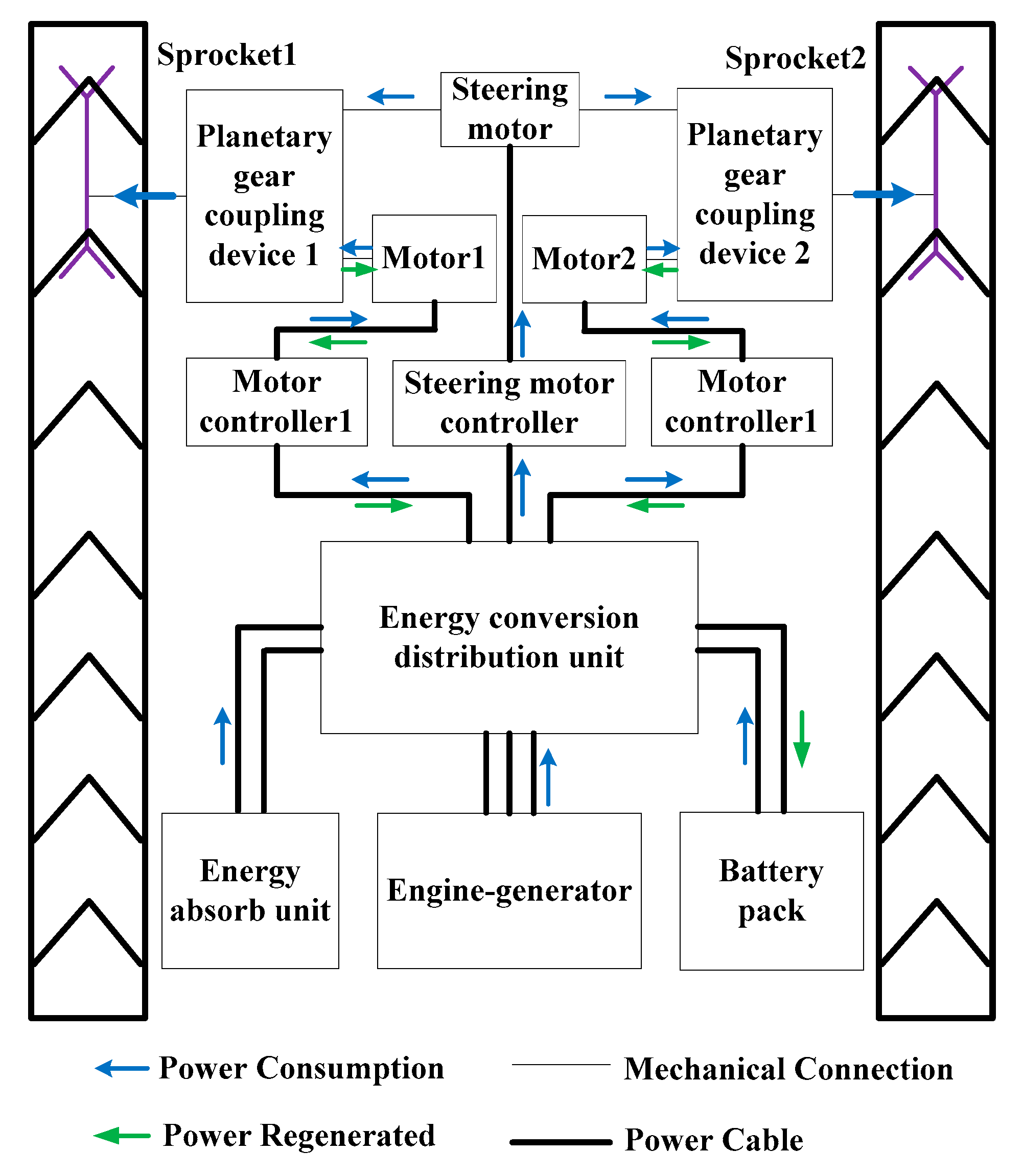
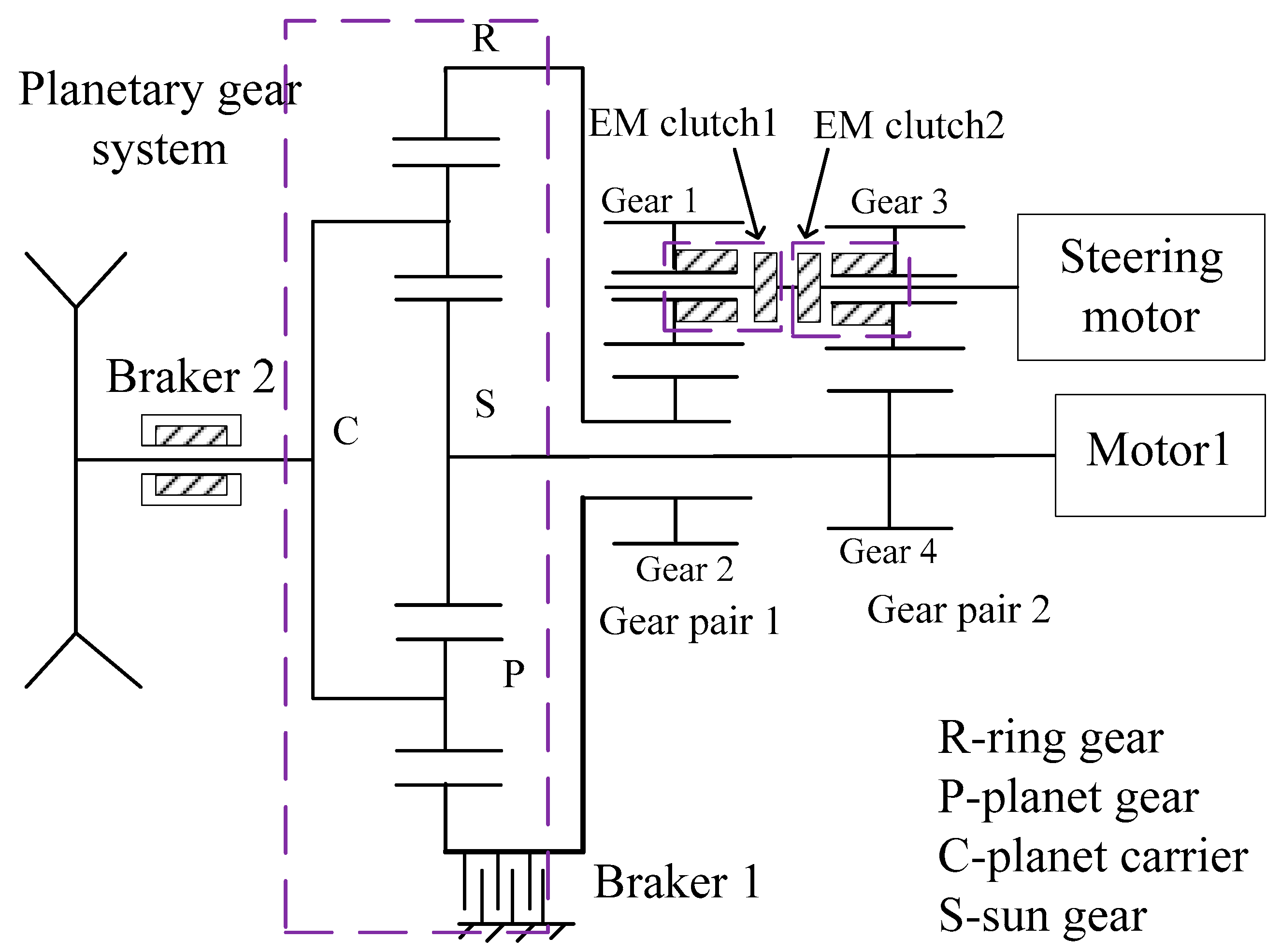
12]. The output torque of the outside sprocket increases with the coupling assembly, but the scheme with two main motors and two auxiliary motors does not reduce the total power requirements for motors in 2MDTVs. A steering coupling system composed of a steering motor, two planetary gear couplers and two propulsion motors is designed to improve the output power [
13]. However the mechanical characteristics of the coupler and the steering performance during high speed were not fully considered.
The steering control of tracked vehicles can be divided into two categories generally: adjusting speed difference between two sprockets based on speed or torque control [
14,
15]. A coordinated hierarchy control strategy of driving torque is proposed for distributed electric drive tracked vehicles [
16]. The quadratic programming method is used to design the torque optimization distribution law of the in-wheel motors. A steering control strategy has been proposed for tracked vehicles propelled by electric transmissions [
17]. The self-adaptive control strategy is designed on the basis of Model Reference Adaptive Control Theory. This strategy could be used to effectively adjust the motors’ driving torques and ensure great steering stability. Some research focus on the energy management strategies of the hybrid electric powertrain to improve the fuel economy [
18]. Algorithms such as Stochastic Dynamic Programming, Radau Pseudospectral Method and Reinforcement Learning are implemented for optimizing the energy management strategy [
19,
20,
21].
However, few studies have focused on the maneuverability and stability of the 2MDTV during high speed steering [
22]. Most of the existing analyses investigate the tracked vehicles without coupling devices during low-speed steering, so the proposed theory and control strategies are only adapted to low-speed steering, and have some limitations for high-speed steering. Due to the absence of the stability control and the shortage of propulsion motor power, the problem of torque allocation for 2MDTVs during steering is still unsolved. In addition, tracks is prone to slip considering the high speed of the vehicle and the adhesion coefficient of the road. At the same time the vehicle is more sensitive to the outside interference caused by the surroundings and pavements, so the vehicle may be out of speed or even roll over if the control system cannot meet the requirements.
In this paper, the impact of efficiency decline is taken into consideration and an electromechanical coupling device is proposed to solve the problem of insufficient power during high-speed steering in curves of different radii. An optimal torque distribution strategy based on torque control considering the slip between track and pavement is proposed to achieve better torque and power utilization. The steering co-simulation model is built by the multi-body software Recurdyn and the control software Matlab/Simulink. A real-time electronic steering control simulation by the Hardware-in-the-Loop (HIL) method verifies the effectiveness of the coupling device and the proposed strategy.
2. Mathematical Model for Steering
The steering of tracked vehicled is achieved by adjusting the speed difference between the two tracks. The electric drive structures of the electric tracked vehicle includes dual-motor independent drive, single motor drive, and hybrid electromechanical complex drive. Dual-motor independent drive structures have been widely used due to their simple structure, high transmission efficiency, flexible layout and other advantages. In this paper, a dual-motor independent drive electric tracked vehicle (2MIETV) is selected, and the vehicle’s configuration is as shown in
Table 1.
The vehicle dynamics performance indicators during straight running are listed as follows:
- (1)
Maximum speed should be 72 km/h.
- (2)
Maximum climbing degree should be 32° and the climbing speed is 18 km/h.
- (3)
Acceleration capability: 0 to 32 km/h in less than 8 s.
The parameters of the propulsion motor can be determined by the above indicators in general [
23], where the transmission efficiency is assumed as a constant value of 0.9. However, the transmission efficiency will decrease while the vehicle speed increases due to the friction loss of crawler mechanism consisting of tracks, sprockets, road wheels, inducers, etc. Then the efficiency of transmission system during the high-speed running can be defined as follows [
24]:
where
ηt is the transmission efficiency,
v is vehicle speed.
In addition, the loss due to internal resistance in crawler mechanism of tracked vehicle cannot be ignored during high-speed driving, and the power consumed by internal resistance in electric tracked vehicles is defined as follows [
25]:
where
Pir is the power consumed by internal resistance in crawler mechanism.
The above power loss described in Equation (2) was not considered in a previous study [
23], and since the output power of propulsion motor cannot satisfy the requirements for high-speed running, the parameters of the drive motor should be determined by consideration of
Pir at high running, as shown in
Table 2.
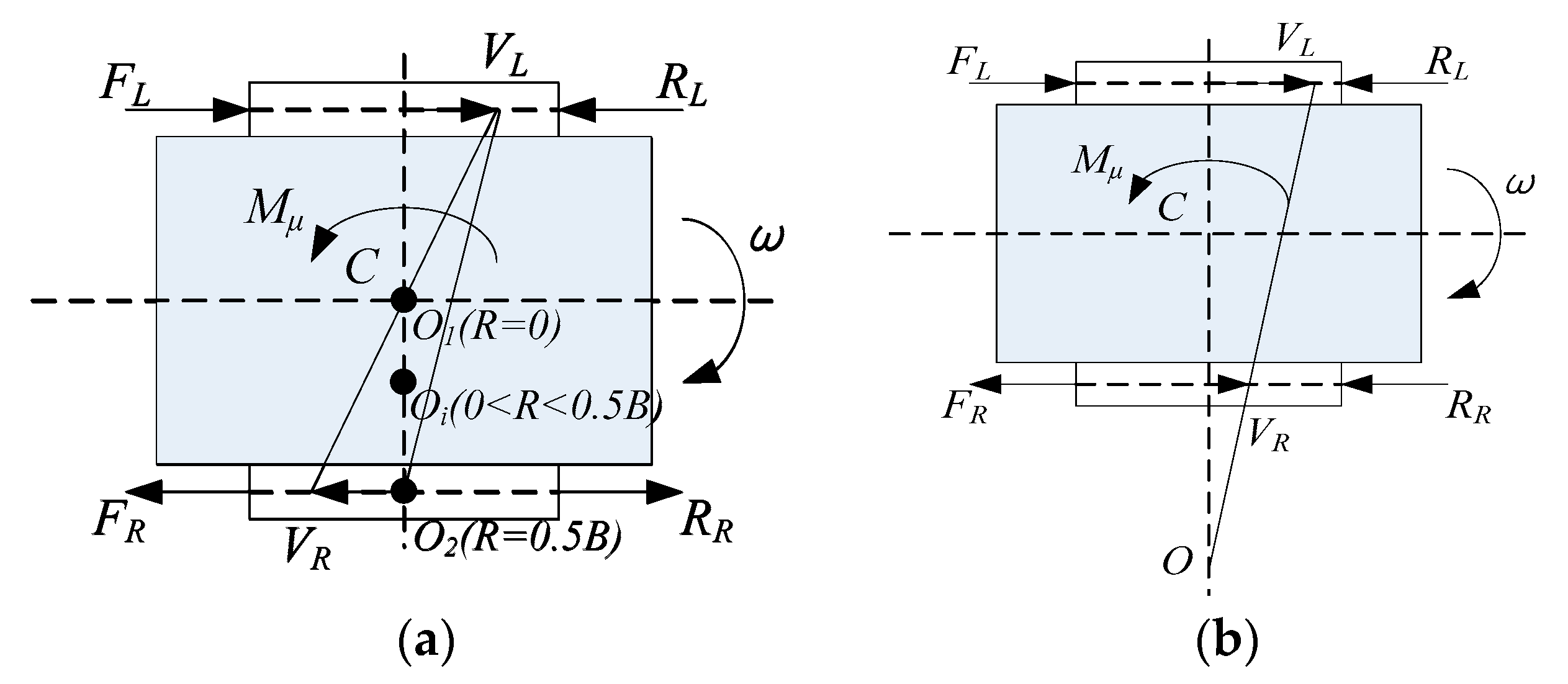
We took right steering as an example,
FL is the traction force on the outer track,
FR is the tractionforce on the inner track,
RL is the rolling resistance force on the outer track,
RR is the rolling resistance on the inner track,
Mμ is the steering resistance moment,
vL is the track speed on the outer side,
vR is the track speed on the inner side and ω is the yaw rate. Steering maneuvers with different radii can be shown in
Figure 1.
Mμ is defined as follows [
26]:
where
μ is the coefficient of roll resistance,
μmax is the maximum rolling resistance coefficient,
R is the steering radius of the vehicle. The rolling resistance of the two tracks is the same in magnitude but opposite in direction when
vR and
vL are opposite in sign. If
vR and
vL are same in sign, the rolling resistance of the two tracks will be the same in direction. The rolling resistance
RL and
RR are expressed as follows:
2.1. Small Radius Steering (R ≤ 0.5B)
This situation can be further divided into three categories:
R = 0, 0 <
R < 0.5
B,
R = 0.5
B. The equilibrium relationship between the force and moment of the vehicle when turning from resting, as shown in
Figure 1a, can be expressed as:
where
FL and
FR are tractive force but opposite in direction.
It’ worth mentioning that when R = 0, FL = FR, VL = VR, lateral acceleration is zero, dv/dt = 0, and when R = 0.5B, VR = 0, RR = 0.
The motor speed on both sides can be expressed as:
where
rz is the radius of the sprocket,
rz = 150 mm
From (1)–(6), the motor torque and power can be obtained as follows:
T is tractive torque but opposite in direction. P is consumed power used to drive the track. Subscript “L” or “R” means the left or right side of the vehicle.
2.2. Big Radius Steering (R > 0.5B)
According to the vehicle dynamic balance, the following formula can be obtained from
Figure 1b:
where
FL is tractive force. In steady-state steering conditions, the expressions of the driving force can be obtained and if we assume the
FR is null:
We thus obtain the solution R = R0 = 67.54 m.
This situation can be also divided into three categories: 0.5B < R < R0, R = R0, R > R0. When R > R0, FR is traction force and is in the same direction with the track. When R = R0, FR = 0, PR = 0. At this moment, the inner propulsion motor is turned off, the track rotates freely, only the outer propulsion motor works. While when R < R0, FR is brake force, generated by motor. The direction between FR and VR is opposite in this situation.
Similarly, during high-speed steering the internal resistance in crawler mechanism increases, so the decline of transmission efficiency cannot be ignored. Therefore, a factor
k is proposed to correct Equation (1). The value of
k, which is determined by simulation or experimental results, ranges from 0.0001 to 0.002:
2.3. Calculation
The steering process can be divided into two periods: dynamic steering and static steering, the motor torque and power required vary with the steering radius and speed. This paper focuses on the steering performance of the vehicle at high speeds. Usually, the yaw rate of ETV is 45~75°/s, we choose
w = 1.3 rad/s. During high-speed steering, in order to prevent the crew from feeling discomfort due to the excessive centripetal acceleration, the centripetal acceleration is limited to 1 g. According to the calculation results, several representative cases are selected, as shown in
Table 3.
It can be seen from
Table 3 that during low-speed small radius steering, the demand torque of the vehicle is large due to the large steering resistance moment, which exceeds the maximum torque that the motor can provide. This has been confirmed in the previous study.
During high-speed steering, the vehicle’s power requirements (60.3/64.2/64.8/66 kW) exceed the maximum power (50 kW) that the motor can provide, so two motors with at least 70 kW are required for a vehicle without a coupling device, whereas during straight driving the required power is only half of the motor maximum power [
4]. If the arrangement with coupling device (50 + 50 + 20 kW) is applied, the peak power will reduce to 20 kW less than the arrangement with two independent propulsion motors (70 + 70 kW). It is noteworthy that the values shown in
Table 3 are calculated with
k = 0. If
k ≠ 0, the lateral power demand can be determined by Equation (11). As
k increases, the power demand actually for the outside motor will be further increased:
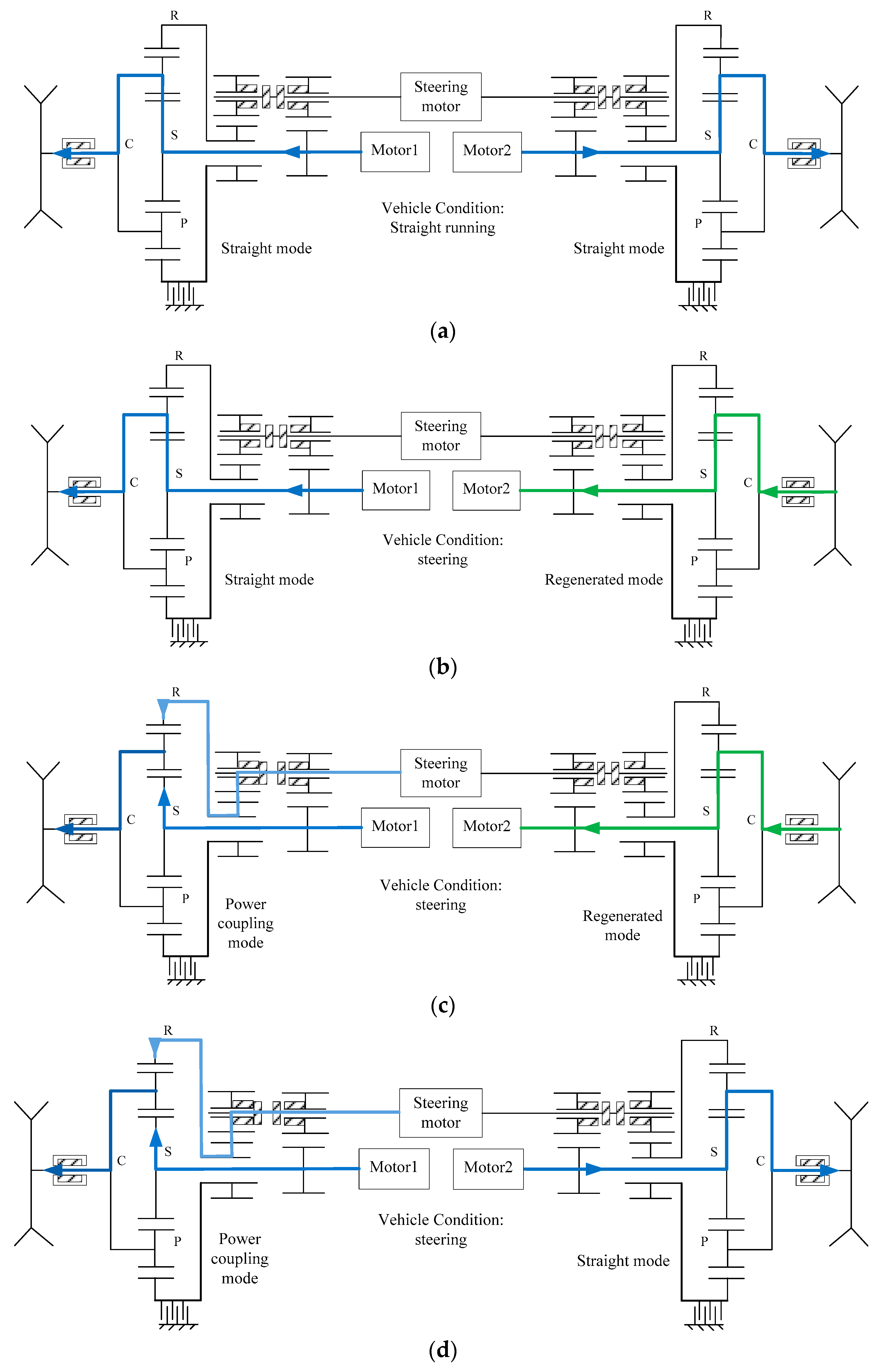
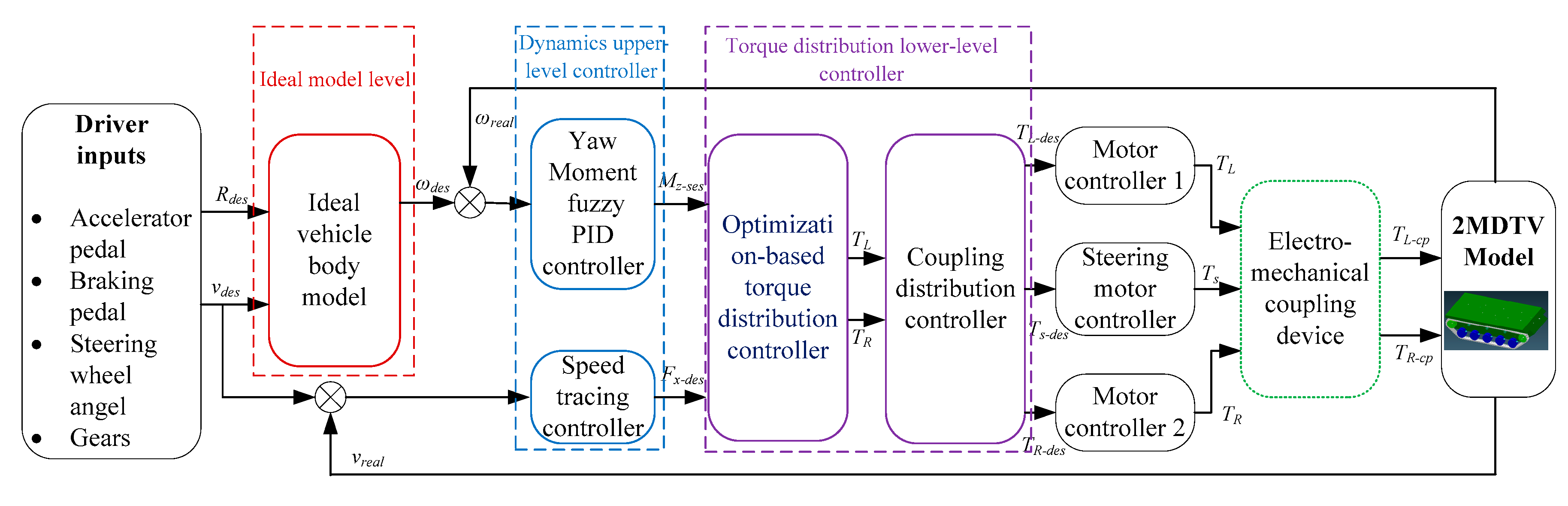
4. Control Strategy
A closed-loop control strategy based on torque control of motor is proposed and shown in
Figure 5. The strategy proposed for a 2MDTV is designed as a three-level structure, including an ideal model level, a dynamics upper-level controller and a torque distribution lower-level controller. In the reference model level, a dynamic reference model is established and discussed in
Section 2 to obtain the desired yaw rate or other dynamics parameters, according to the driver inputs and the actual state of the vehicle. The upper-level controller consists of a speed tracking controller and a yaw moment controller with the PID control method and fuzzy PID control, respectively. The controller in this level aims to guarantee the capability of speed following and basic steering performance. The lower-level controller adopts the optimal allocation algorithm to assign the optimal torque (
TL,
TR) to desired torque (
TL-des,
Ts-des,
TR-des) generated by propulsion motors and steering motor under the constraints of the planetary coupling device. Based on the above calculation, the output torque of two propulsion motors and steering motor can be directly distributed to three motor controllers by a CAN bus, respectively. Finally, the torque or power is coupled through the electromechanical coupling device and transmitted to sprockets to improve the stability of the 2MDTV.
4.1. Yaw Moment Fuzzy PID Controller
The yaw moment controller is designed based on the error between the actual angular speed and the desired angular speed to calculate the target yaw moment Mz-des by the fuzzy PID control method. This controller is activated when the yaw rate error Δω beyond the constant 0.1.
4.2. Speed Tracing Controller
The speed tracking controller is always activated and designed based on the PID control method to calculate the desired traction force of vehicle Fx-des for the purpose of following the desired vehicle speed. Usually during high speed steering, the speed of the vehicle declines rapidly and the steering mode is translated into low speed steering, so the speed tracking controller is important especially for high speed steering.
4.3. Optimization-Based Distribution Controller
To improve the performance of the speed and yaw rate following, an optimization-based distribution controller is designed to obtain the optimal torque
TL and
TR of the bilateral sprockets. According to
Figure 5, the torque
TL,
TR and
Ts, which are supposed to be generated by propulsion motors and steering motor, are allocated by the coupling distribution controller under the constraint of planetary coupling to track desired steering radius.
The rolling resistance is assumed to be zero and then the matrix form
H can be obtained according to the dynamic balance analysis in
Section 2 and expressed as follows:
where:
,
.
where
κ are the control inputs,
u are the torque of the sprockets, and
H, the control effectiveness matrix, is chosen depending on the steering radius. The optimization object to minimize is chosen as distribution error,
, for control accuracy and
u, for efficient driving. We thus obtain the optimization objective function:
This is a weighted least-squares (WLS) problem, and where
Wu is the weighting matrix for efficient driving,
Wv is the diagonal weighting matrix of the inputs,
is the weighting factor whose value is chosen depending on how important the distribution error is. The objective function is determined by the following constraints:
where
ε is the efficiency of motor obtained by map diagram of speed-torque.
4.4. Coupling Distribution Controller
The coupling distribution controller allocate the torque
TL,
TR and
Ts according to the torque
TL and
TR received form the optimization-based distribution controller in different situations. The torque distribution is based on following constraints:
In order to reduce the complexity of the control system, the priority for dual motor operating mode is the highest. The desired torque (
TL-des,
Ts-des,
TR-des) can be obtain according to Equation (15) and coupling judgment module [
23]. The steering motor works only when the propulsion motor can’t generate enough torque or power during some steering situations.
5. Modeling and Simulation Results
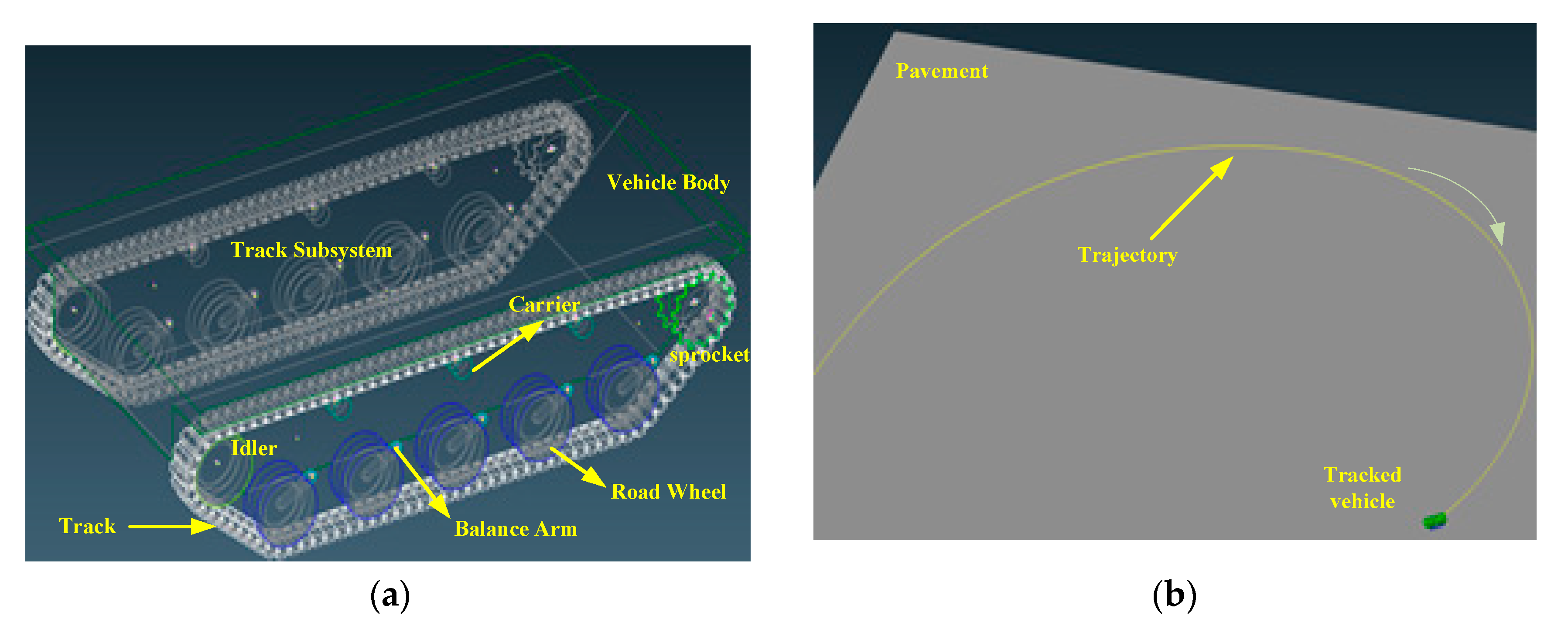
We build the steering co-simulation model using the multi-body software Recurdyn and control software Matlab/Simulink. The vehicle model and ground model are developed in Recurdyn, as shown in
Figure 6. The driver inputs model, the control strategy model and the motor system model are developed in Simulink. The multi-body dynamic model in Recurdyn is seamlessly interfaced with Matlab/Simulink. The parameters of the dynamic simulation parameters are shown in
Table 5.
The RecurDyn software can define soil parameters according to the user’s needs. The road is divide into rectangular elements for calculation. Therefore, the contact force between the track and the ground can be automatically calculated by the software. The calculation is based on the following two models: a hard pavement model established by general contact force, and a soft pavement model based on Baker’s theory. We choose the hard pavement model in this paper.
The pressure between the track shoes and the ground on hard pavement is defined by the track contact. The contact-collision force in RecurDyn is calculated as:
where
q is ground contact position before contact,
q0 is ground contact position after contact,
q −
q0 is the subsidence.
According to relevant theories and experiments, the convergence speed of the simulation is obtained optimally when the soil deformation index n is ranged from 2 to 3. The friction between the track and the ground is calculated by Coulomb’s law. The parameters of the hard pavement used in the simulation are shown in
Table 6.
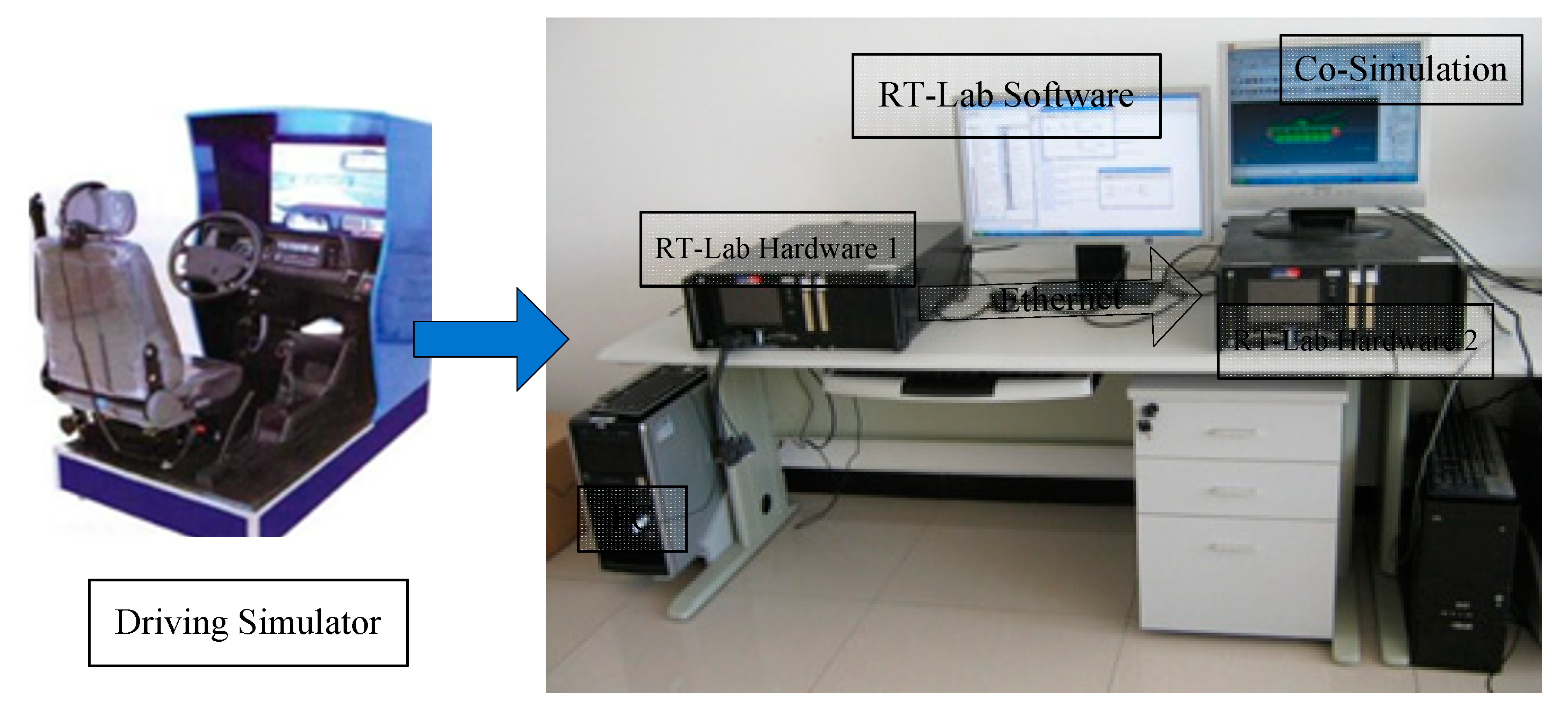
A real-time electronic steering control simulation by the Hardware-in-the-Loop (HIL) method is constructed with rapid simulation prototyping technology, as shown in
Figure 7. The Simulink models of electronic differential steering control strategy and motor control strategy are compiled into executable codes via RT-LAB software. Then the executable codes are loaded to RT-LAB hardware 1 and RT-LAB hardware 2 respectively to run the real-time simulation. The required output torque signal of four motors obtained from HIL simulation of ECU are input to RT-LAB hardware 2 for HIL simulation of motors. The output torque signals from HIL simulation of motors are given to the Simulink vehicle model built by Recurdyn. Some typical high-speed steering cases are simulated to verify the feasibility of the coupling device and the strategy proposed.
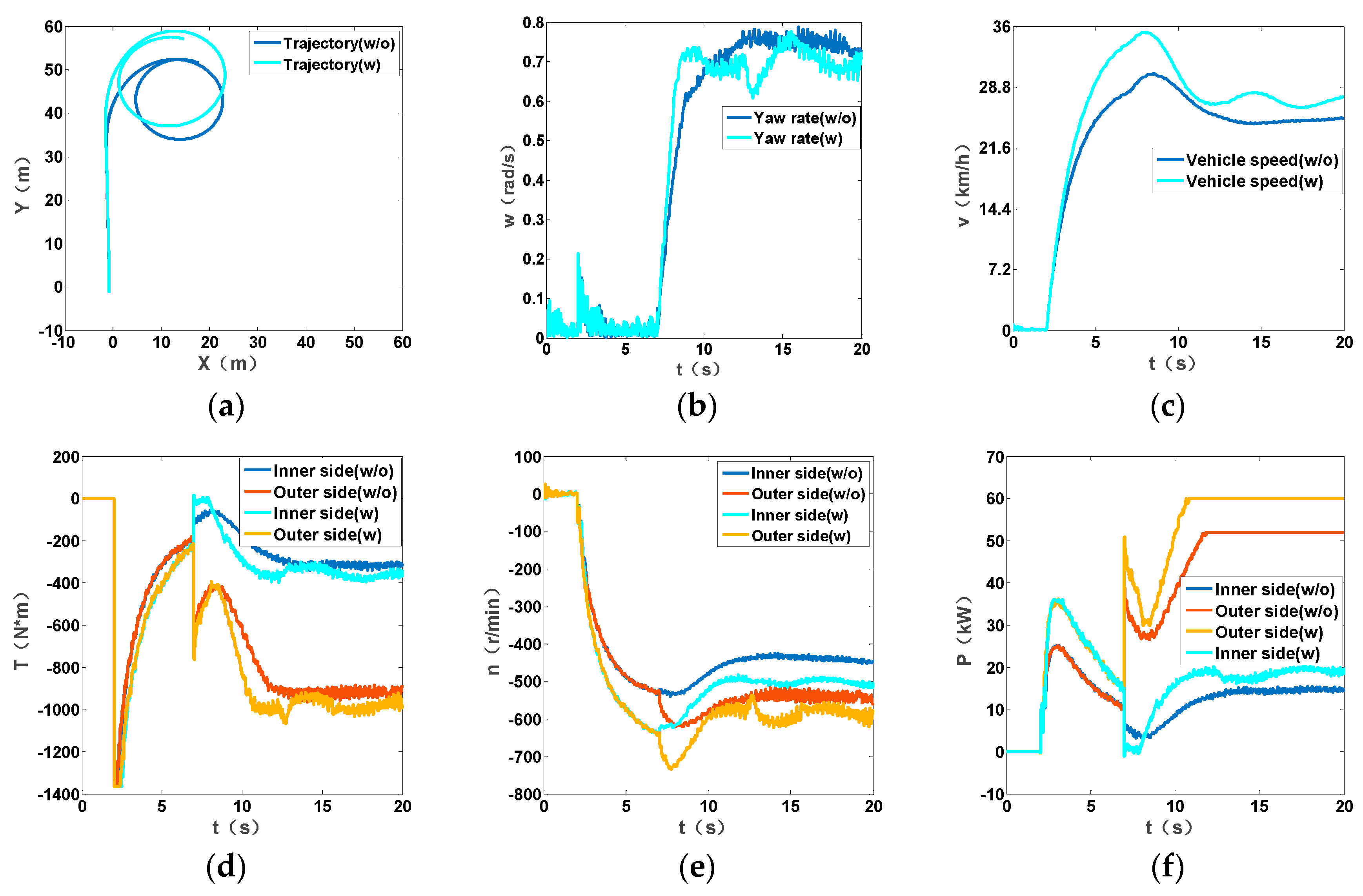
5.1. 5B Steering
At first, the vehicle is stationary for 2 s. After that, the vehicle starts running straight for 5 s and accelerates to 28.8 km/h. The steering wheel is turned to the right at 7 s and manipulated to output
R = 5
B. The trajectory, yaw rate and speed of the vehicle are shown in
Figure 8a–c. Without the coupling system, the vehicle speed declines continually, while with the coupling device the vehicle speed is higher, which can maintain near the theoretical value, as shown in
Figure 8c. The torque, rotation speed and power of the sprocket are shown in
Figure 8d–f. Limited by the motor power, the speed of the sprocket is lower without the coupling device.
Figure 8f shows that the output power of outer sprocket is improved from 50 to 60 kW, and the vehicle speed can be maintained with the coupling device. It is worth mentioning that, seen from
Figure 8b, the yaw rate of the vehicle cannot be too large during high speed steering, and otherwise the vehicle is easy to be instability or rollover. Although the yaw rate is lower than what we assumed, but at this situation the power demand is still high (larger than the calculated value).
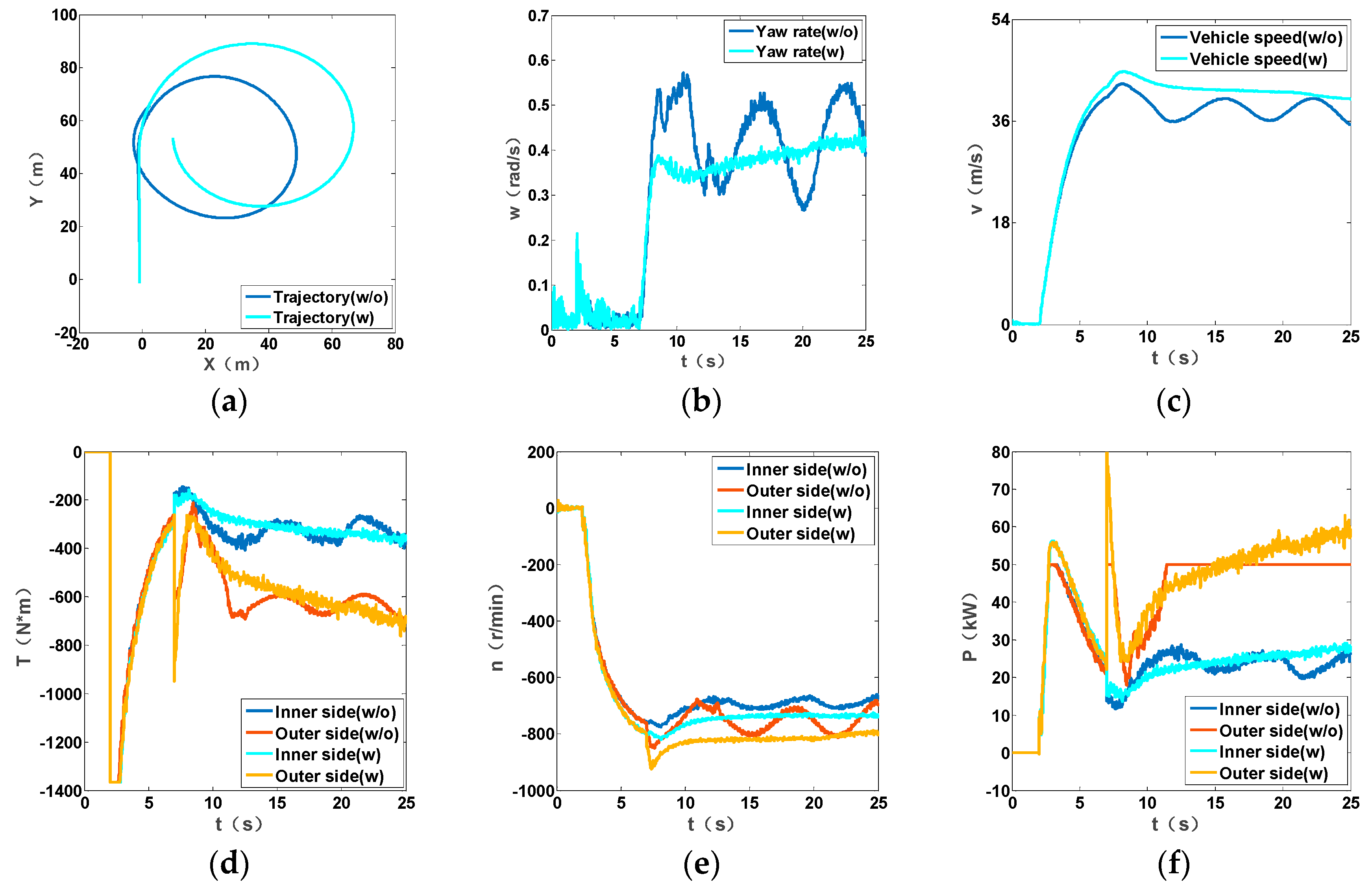
5.2. 10B Steering
At first, the vehicle is stationary for 2 s. After that, the vehicle starts running straight for 5 s and accelerates to 40.7 km/h. The steering wheel is turned to the right at 7 s and manipulated to output
R = 10
B. The trajectory, yaw rate and speed of the vehicle are shown in
Figure 9a–c. From
Figure 9b we know that without the coupling device, the fluctuation of the vehicle yaw rate deteriorate the trajectory controllability, also the vehicle speed fluctuates and declines at the same time. While the speed of the vehicle with coupling device is close to the target value. The torque, rotation speed and power of the sprocket are shown in
Figure 9d–f. The graph shows that the torque varies smoothly with the coupling device. Without the coupling device, the rotation speed is lower and there are fluctuations due to the limitation of the motor power according to
Figure 9e. However, the output power increases with the coupling device, therefore the vehicle can turn in high speed. It is worth noting that the yaw rate is a little lower to ensure the stability of the vehicle, however, the power demand is still quite high especially during dynamic steering.
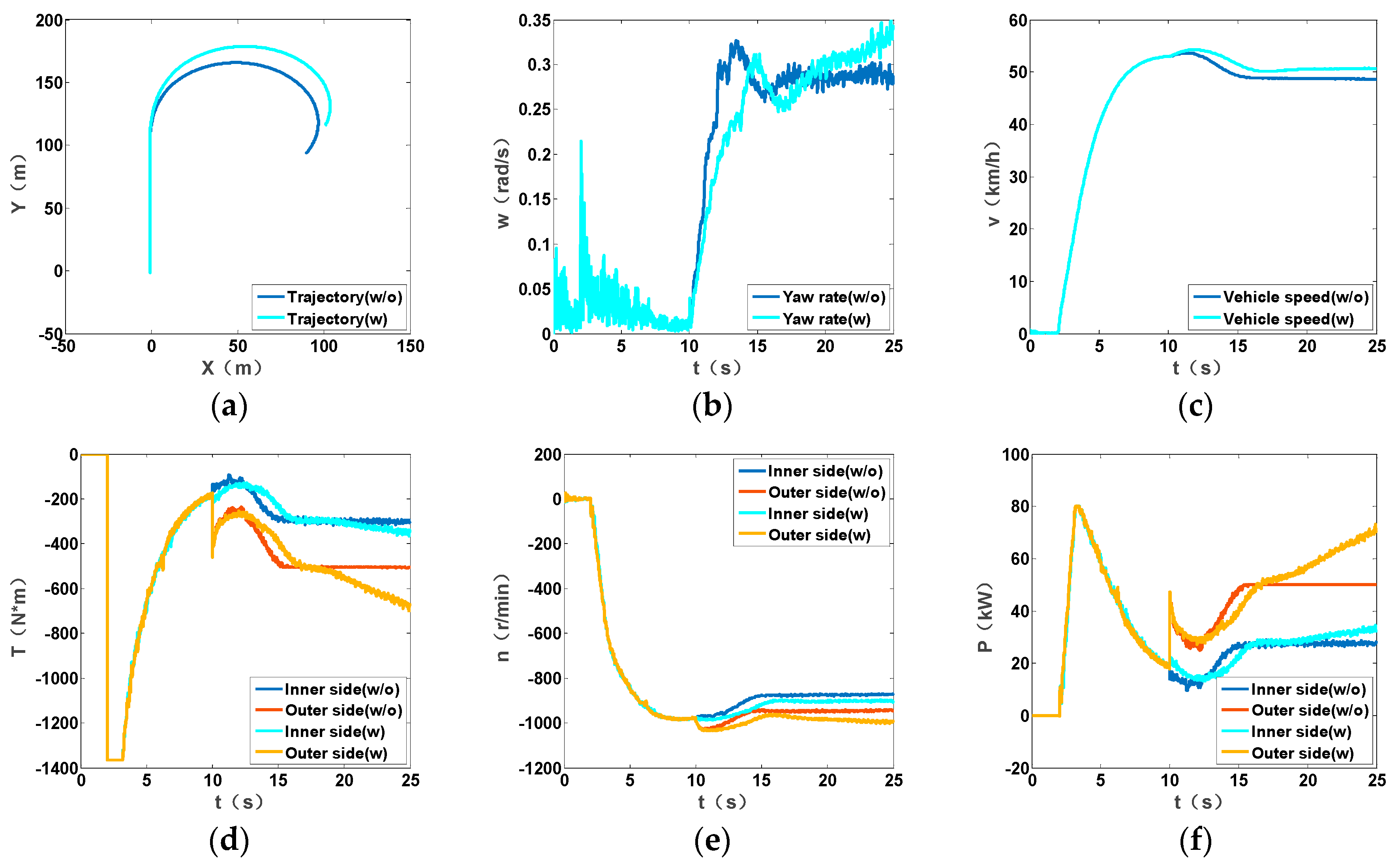
5.3. 20B Steering
At first, the vehicle is stationary for 2 s. After that, the vehicle starts running straight for 8 s and accelerates to 57.5 km/h. The steering wheel is turned to the right at 10 s and manipulated to output
R = 20
B. The trajectory, yaw rate and speed of the vehicle are shown in
Figure 10a–c. We can see from
Figure 10a that the steering radius is quite large due to the slip between tracks and the ground during high-speed steering. To avoid the rollover or instability of the vehicle, the yaw rate is not as high as the value we assumed. However, the yaw rate of the vehicle with coupling device is still higher. The vehicle speed is higher with the coupling device while 11% lower than the theoretical value according to
Figure 10c. The torque, rotation speed and power of the sprocket are shown in
Figure 10d–f. It can be seen that the output torque and the speed of the sprocket are not changed greatly during stationary steering due to the limitation of the motor power. The output torque and the speed of the sprocket is lower without the coupling device. While with the coupling device the output power is improved and the vehicle speed can be maintained at higher level. Although the yaw rate is not large, the power demand is still larger than the calculated value to maintain the high speed during steering.
6. Conclusions
In this paper, according to the dynamic analysis of the 2MDTV, we found that the power required by the propulsion motor is quite large during high-speed steering situations. As the existing research focused more on low-speed conditions, we considered the vehicle performance during high speed steering in this work and supplemented the calculations about the power demand. In order to solve the problem of understeer and speed decline of the vehicle caused by insufficient power during high speed steering, a new electromechanical coupling device is proposed. The device is used to couple the power of the steering motor and the propulsion motor to satisfy the requirements for high-speed steering. The coupling system can increase the power of outer track by 20 kW during high-speed steering. Furthermore, an optimized torque distribution control strategy is proposed. In the Hardware-in-the-Loop (HIL) simulation of 5B, 10B, and 20B steering with RecurDyn and Matlab/Simulink models, the coupling device can improve the output power of the vehicle, and the proposed strategy can improve the steering stability and achieve smoother steering response of the vehicle at high speed.


