An Optimization Method for Local Consumption of Photovoltaic Power in a Facility Agriculture Micro Energy Network

Abstract
:
1. Introduction
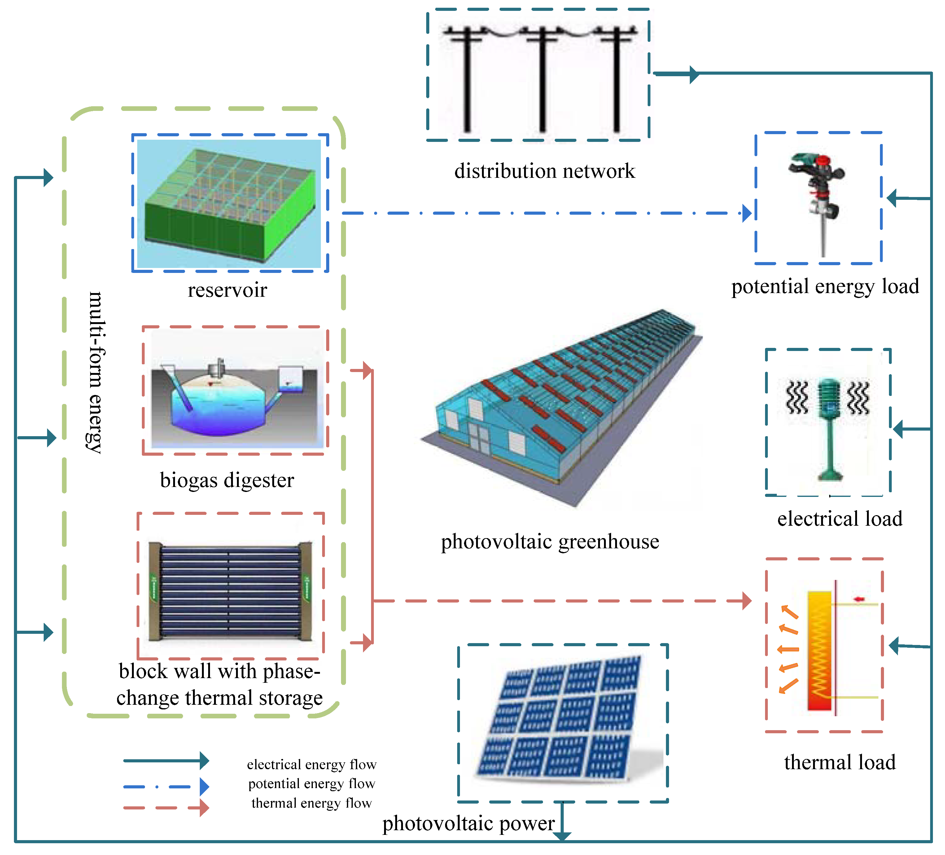
2. Typical Structure of Photovoltaic Greenhouse Facility Agricultural Micro Energy Network System
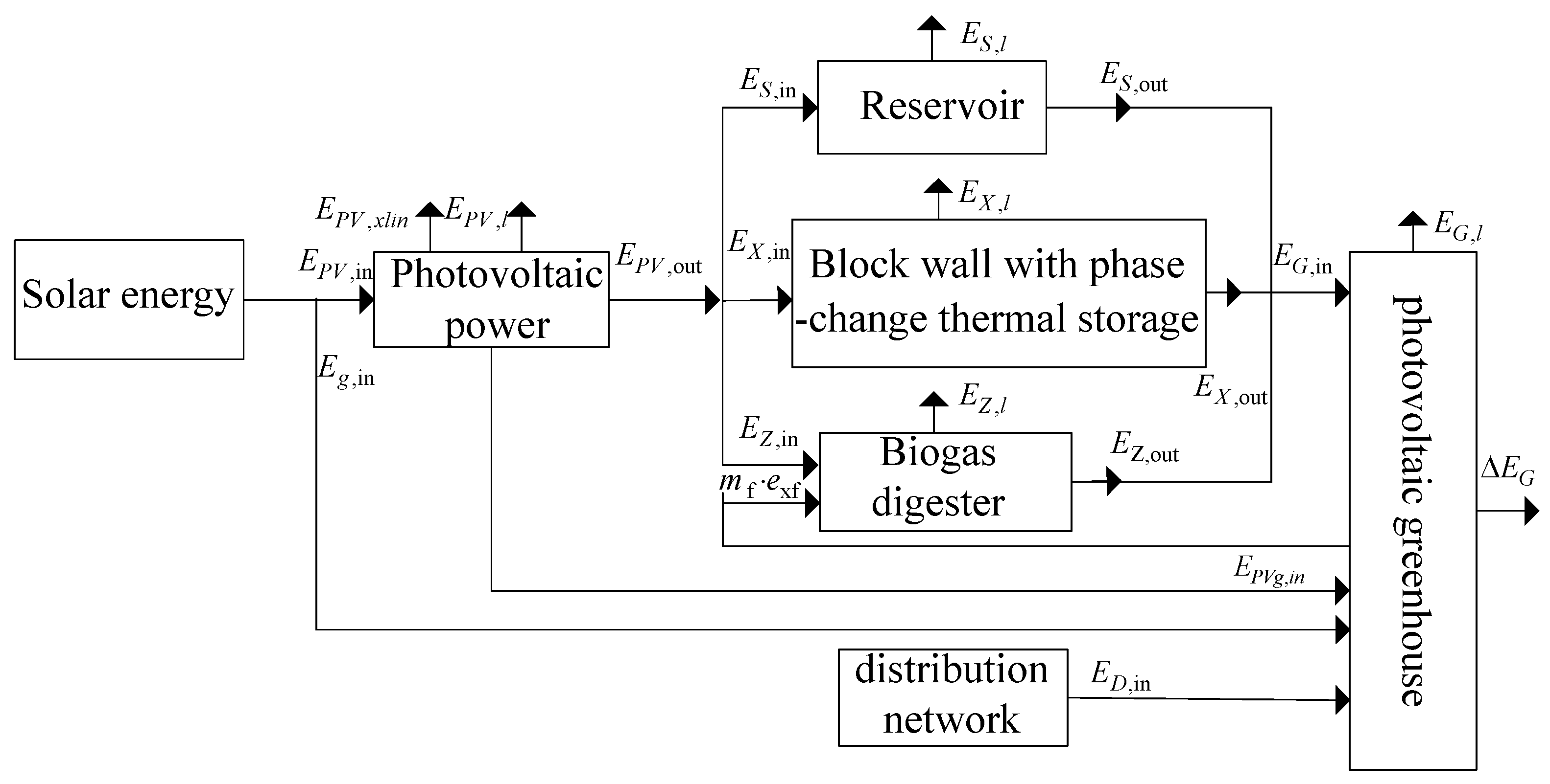
3. Multiform Energy Storage Input-Output Power Model
- (1)
- Reservoir energy input-output power model
- (2)
- Reservoir energy input-output power model
- (3)
- Block wall with phase-change thermal storage energy input-output power model
4. Optimal Energy Dispatching Model for Facility Agriculture Micro Energy Network Systems with Photovoltaic Greenhouses
4.1. Objective Function
4.2. Constraints
- (1)
- Energy balance constraint
- (2)
- Multiform energy storage space constraint
- (3)
- Time-shiftable load continuity work status constraint
- (4)
- Time-shiftable load non-working time constraint
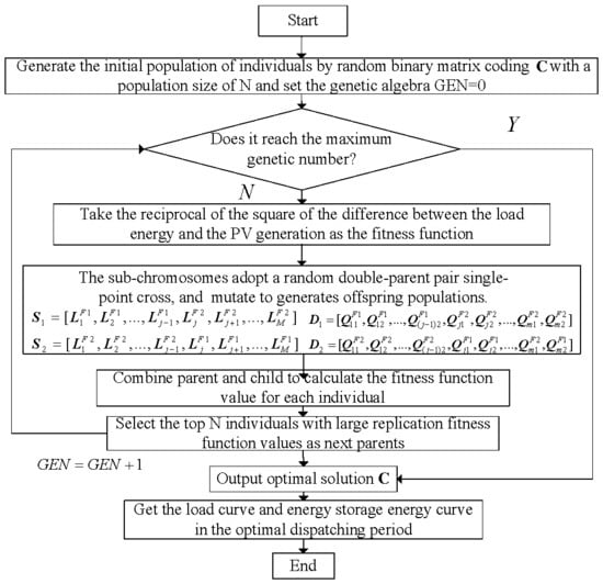
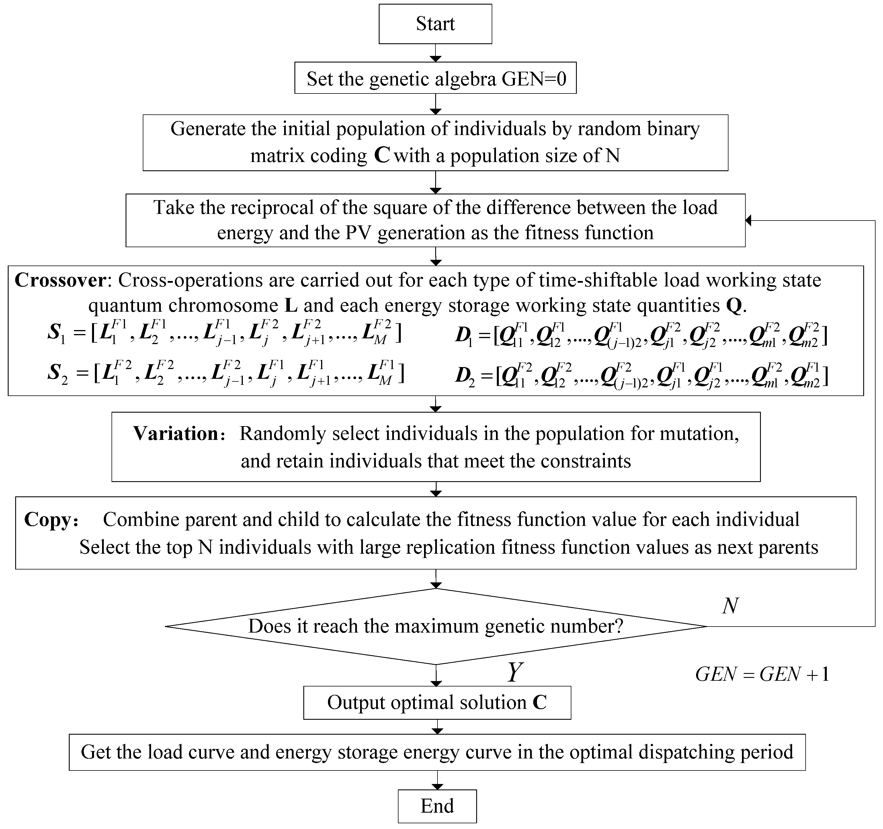
5. Solution of the Optimal Dispatching Model Based on a Genetic Algorithm with Matrix Binary Coding
5.1. Matrix Binary Coding of Control Variables
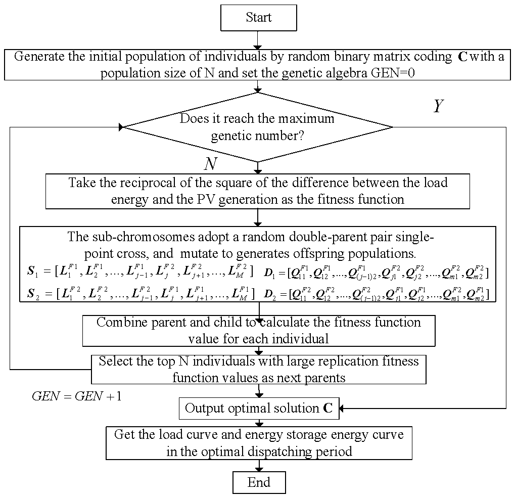
5.2. Genetic Algorithm Solution Process
- (a)
- Generate a random crossover position j between 1 and M.
- (b)
- Perform a crossover on the two column vectors at crossover position j to generate the new sub-chromosomes , :
- (a)
- Generate a random crossover position j between 1 and m.
- (b)
- Perform a crossover operation on the two column vectors at crossover position j to generate the the new sub-chromosomes and :
6. Examples
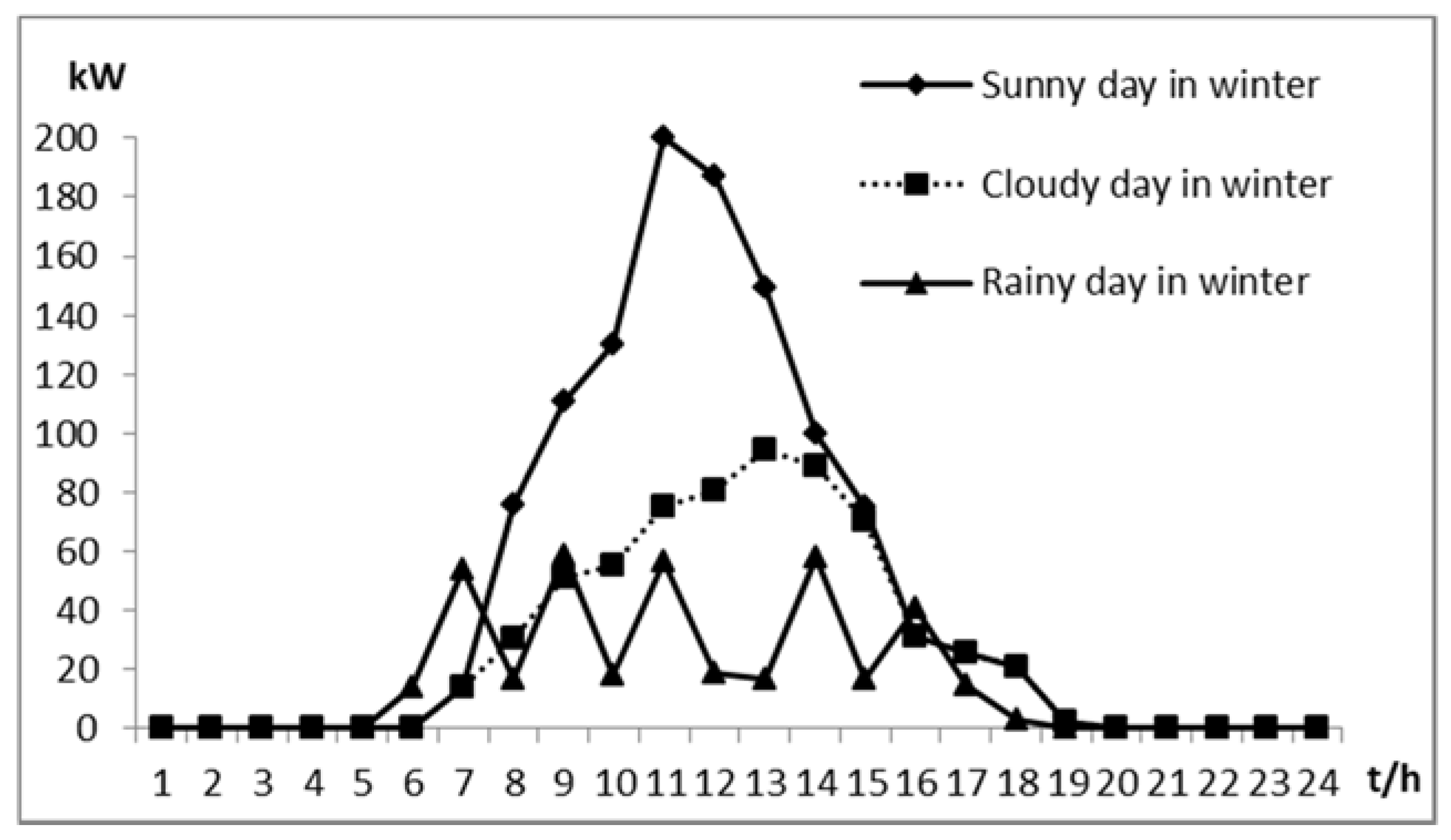
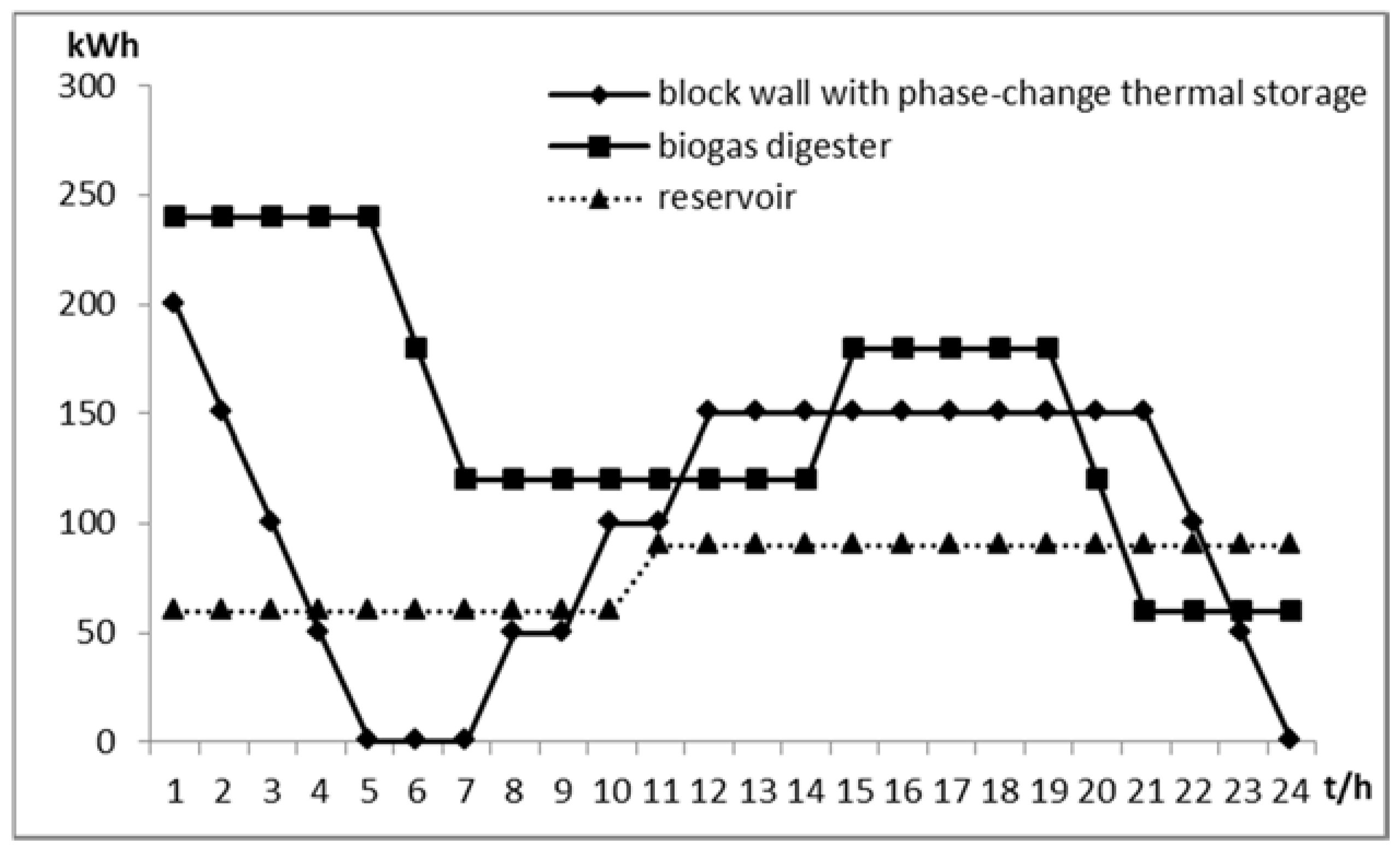
6.1. Basic Information
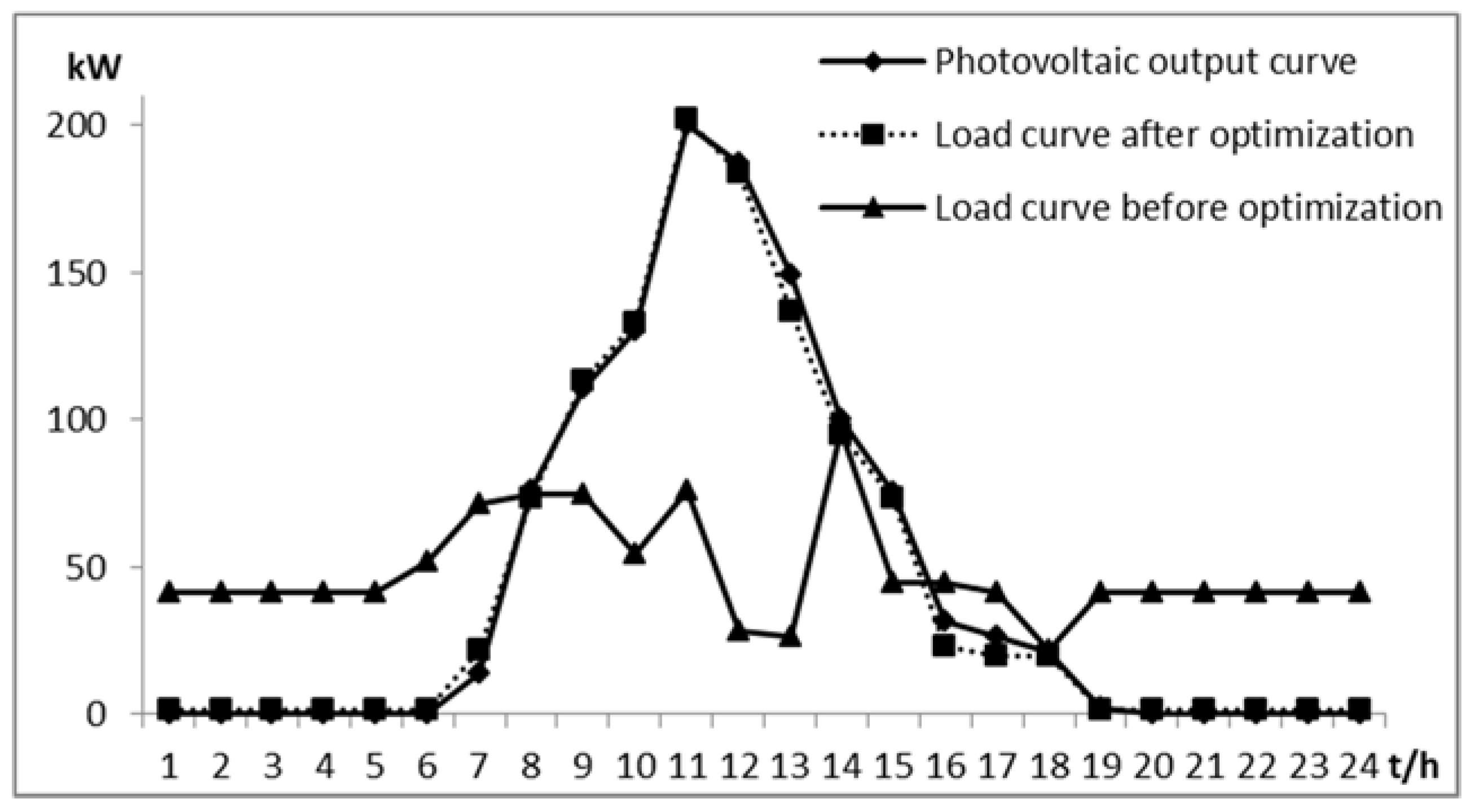
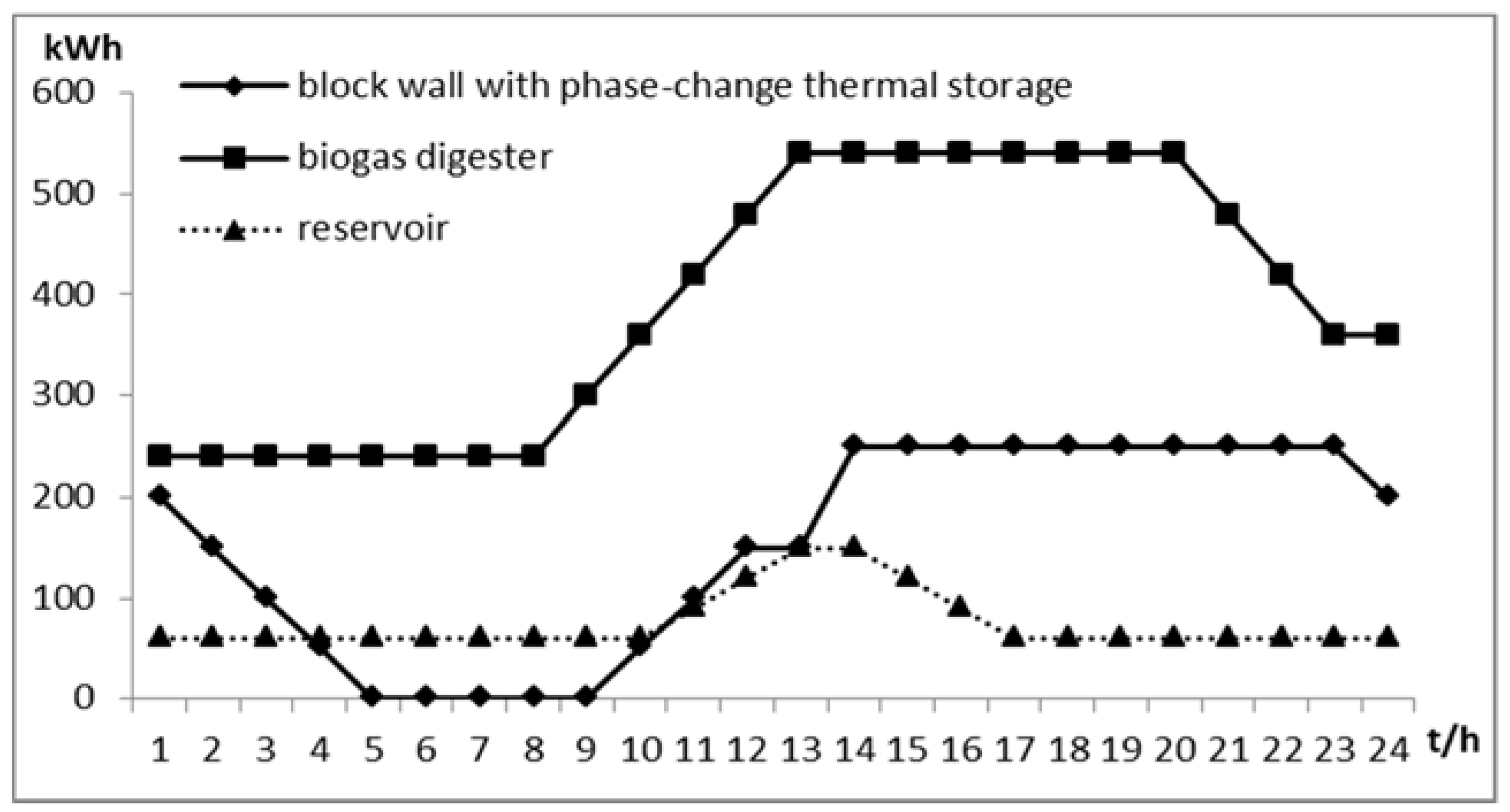
6.2. Analysis of Examples
7. Conclusions
Author Contributions
Acknowledgments
Conflicts of Interest
References
- National Energy Administration. The State Council Leading Group Office of Poverty Alleviation and Development. In Engineering Work Plan about Implementing PV Poverty Alleviation; National Energy Administration: Beijing, China, 2014. [Google Scholar]
- Wang, X. Tension and Digestion in the Process of Precise Poverty Alleviation Policy in Contiguous. Master’s Thesis, Shangdong University, Jinan, China, 2017. [Google Scholar]
- Xu, B. Research on the Implementation of the Policy of Precise Poverty Alleviation in Jining, Shangdong. Master’s Thesis, Northeast Agricultural University, Harbin, China, 2017. [Google Scholar]
- Cho, H.; Smith, A.D.; Mago, P. Heating cooling heating and power: A review of performance improvement and optimization. Energy 2014, 136, 168–185. [Google Scholar]
- Rafiee Sandgani, M.; Sirouspour, S. Priority-based Microgrid Energy Management in a Network Environment. IEEE Trans. Sustain. Energy 2018, 9, 980–990. [Google Scholar] [CrossRef]
- Peacock, A.D.; Newborough, M. Impact of micro-combined heat-and-power system on energy flows in the UK electricity supply industry. Energy 2006, 31, 1468–1482. [Google Scholar] [CrossRef]
- Werth, A.; Kitamura, N.; Tanaka, K. Conceptual study for open energy systems: Distributed energy network using interconnected dc nanogridsWerth. IEEE Trans. Smart Grid 2015, 6, 1621–1630. [Google Scholar] [CrossRef]
- Vesterlund, M.; Toffolo, A.; Dahl, J. Simulation and analysis of a meshed district heating network. Energy Convers. Manag. 2016, 122, 63–73. [Google Scholar] [CrossRef]
- Vesterlund, M.; Dahl, J. A method for the simulation and opti-mization of district heating systems with meshed networks. Energy Convers. Manag. 2015, 89, 555–567. [Google Scholar] [CrossRef]
- Tao, Z.; Fuxing, Z.; Yan, Z. Study on energy management system of energy internet. Power Syst. Technol. 2016, 40, 146–155. [Google Scholar]
- Tianqi, L.; Donglin, J. Economic operation of microgrid based on operation mode optimization of energy storage unit. Power Syst. Technol. 2012, 36, 45–50. [Google Scholar]
- Yulong, H.; Chunjuan, J.; Yuankui, F. Research on capacity allocation and economy of islanded microgrid. In Proceedings of the 2017 IEEE Transportation Electrification Conference and Expo, Asia-Pacific (ITEC Asia-Pacific), Harbin, China, 7–10 August 2017. [Google Scholar]
- Hao, X.; Wei, P.; Yanhong, Y.; Zhiping, Q.; Li, K. Energy storage capacity optimization for microgrid considering battery life and economic operation. High Volt. Eng. 2015, 41, 3256–3265. [Google Scholar]
- Dan, X.; Qiang, D.; Yi, P. Study on optimizing capacity of storage battery in microgrid system based on economic dispatch. Power Syst. Prot. Control 2011, 39, 55–59. [Google Scholar]
- Xueting, Z.; Tianqi, L.; Qian, L. A dynamic peak load regulation margin based coordinated optimal dispatching under grid-connection of wind farm. Power Syst. Technol. 2015, 39, 1685–1690. [Google Scholar]
- Dany, G. Power reserve in interconnected systems with high wind power production. IEEE Porto Power Tech Proc. 2001, 4, 10–13. [Google Scholar]
- Tiejiang, Y.; Qin, C.; Yibulayin, T.; Yiyan, L. Optimized economic and environment-friendly dispatching modeling for large scale wind power integration. Proc. CESS 2010, 30, 7–13. [Google Scholar]
- Dongfeng, Y.; Suquan, Z.; Feng, B. Analysis on peak load regulation capability of power grid integrated with wind farms in valley load period. Power Syst. Technol. 2014, 38, 1446–1451. [Google Scholar]
- Carpinelli, G.; Mottola, F.; Proto, D. Optimal scheduling of a microgrid with demand response resources. IET Gener. Transm. Distrib. 2014, 8, 1891–1899. [Google Scholar] [CrossRef]
- Xiang, Y.; Liu, J.; Liu, Y. Robust energy management of microgrid with uncertain renewable generation and load. IEEE Trans. Smart Grid 2016, 7, 1034–1043. [Google Scholar] [CrossRef]
- Mehdizadeh, A.; Taghizadegan, N. Robust optimisation approach for bidding strategy of renewable generation-based microgrid under demand side management. IET Renew. Power Gener. 2017, 11, 1446–1455. [Google Scholar] [CrossRef]


| Load Names | Uses | Load Characteristics |
|---|---|---|
| LED plant growth lighting | Increase production | Time-shiftable electric load |
| Plasma nitrogen fixation and water treatment | Increase production and prevent diseases | Time-shiftable electric load |
| Biogas heat pump | Biogas production | Time-shiftable heat load |
| Far infrared heating | Insulation | Time-shiftable heat load |
| Greenhouse heat pump storage system of phase-change | Insulation | Time-shiftable heat load |
| Physical insecticide | Organic agriculture | Time-shiftable electric load |
| Irrigation watering | Organic agriculture | Time-shifted potential energy load |
| Space electric field | Purify and increase production | Non-time-shiftable electric load |
| Rolling shutter motor | Insulation | Non-time-shiftable electric load |
| Shed lighting | Daily work | Non-time-shiftable electric load |
| Smart agricultural monitoring and control system | Monitoring control | Non-time-shiftable electric load |
| Plant nutrient recycling | Sterilization | Non-time-shiftable electric load |
| Sound waves encourage | Increase production | Time-shiftable electric load |
| Ventilator | ventilation | Non-time-shiftable electric load |
| Load | Power kW | Workable Hours | Work Time before Optimization | Work Time after Optimization |
|---|---|---|---|---|
| ventilator | 20 | 0–23 | 8; 9; 12–17 | 10–16 |
| LED growth lighting | 50 | 6–20 | 6–11; 14 | 8; 9; 11–15 |
| Plasma nitrogen fixation and water treatment | 20 | 0–23 | 12; 14 | 7; 11 |
| Plant nutrient recycling | 2 | 0–23 | 10–12 | 12–14 |
| Sound waves encourage | 3 | 0 -23 | 7–9; 14–19 | 8–16 |
| Physical insecticide | 1.5 | 0–23 | 12; 13 | 11; 12 |
| Far infrared heating | 40 | 0–23 | 0–5; 20–23 | 0–5, 24 phase change heat storage heat pump works to provide heat; 20–23 biogas combustion provides heat |
| Irrigation watering | 20 | 10 -17 | 14–17 | 14–17 Water Storage Irrigation Water Potential Energy |
| Reservoir pump input | 30 | 0–23 | -- | 10–13 |
| Biogas pump heat pump input | 60 | 0–23 | -- | 9–11; 13 |
| Phase change heat storage heat pump input | 50 | 0–23 | -- | 8–12 |
| Load | Power kW | Workable Hours | Work Time before Optimization | Work Time after Optimization |
|---|---|---|---|---|
| Far infrared heating | 40 | 0–23 | 0–6; 19–23 | 0–4, 21–23 phase change heat storage heat pump works to provide heat; 5–6, 19–20 biogas combustion provides heat |
| Reservoir pump input | 30 | 0–23 | -- | 10 |
| Biogas pump heat pump input | 60 | 0–23 | -- | 14 |
| Phase change heat storage heat pump | 50 | 0–23 | -- | 7; 9; 11; 16 |
| Load | Power kW | Workable Hours | Work time before Optimization | Work Time after Optimization |
|---|---|---|---|---|
| Ventilator | 20 | 0–23 | 12–17 | 9; 11; 12; 15; 17; 18 |
| Far infrared heating | 40 | 0–23 | 0–6; 19–23 | 0–3; 22; 23 phase change heat storage heat pump works to provide heat; 4–6; 19–21; biogas combustion provides heat |
| Reservoir pump input | 30 | 0–23 | -- | 8; 9; 13; 14; 16 |
| Biogas pump heat pump input | 60 | 0–23 | -- | 12; 13 |
| Phase change heat storage heat pump input | 50 | 0–23 | -- | 10; 11; 14; 15 |
| Load | Power kW | Workable Hours | Work time before Optimization | Work Time after Optimization |
|---|---|---|---|---|
| Ventilator | 20 | 0–23 | 12–17 | 7; 11; 12; 15; 17; 18 |
| Far infrared heating | 40 | 0–23 | 0–6; 19–23 | 0; 19–21; 23 phase change heat storage heat pump works to provide heat; 22 biogas combustion provides heat |
| Reservoir pump input | 30 | 0–23 | -- | 8; 13; 16 |
| Biogas pump heat pump input | 60 | 0–23 | -- | 12; 13 |
| Phase change heat storage heat pump input | 50 | 0–23 | -- | 9–11; 15 |
| Scenarios | Consumption before Optimization | Percentage of Consumption before Optimization | Consumption after Optimization | Percentage of Consumption after Optimization | Percentage of Increase in Consumption before and after Optimization |
|---|---|---|---|---|---|
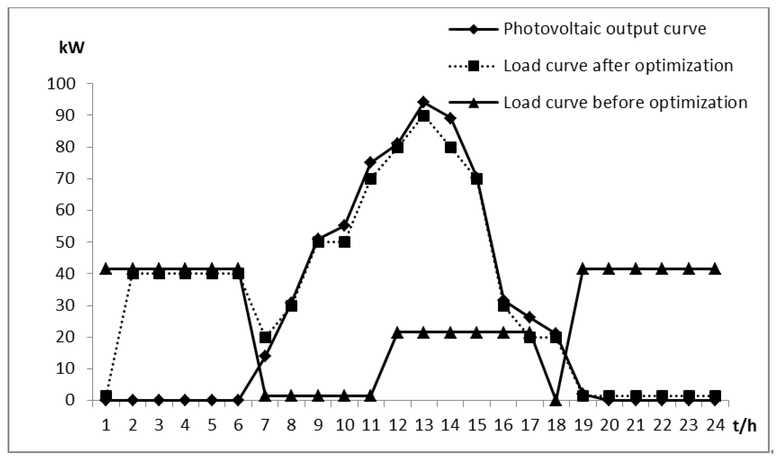
| Sunny day | 491.3 kWh | 43.7% | 1077.7 kWh | 96.1% | 52.4% |
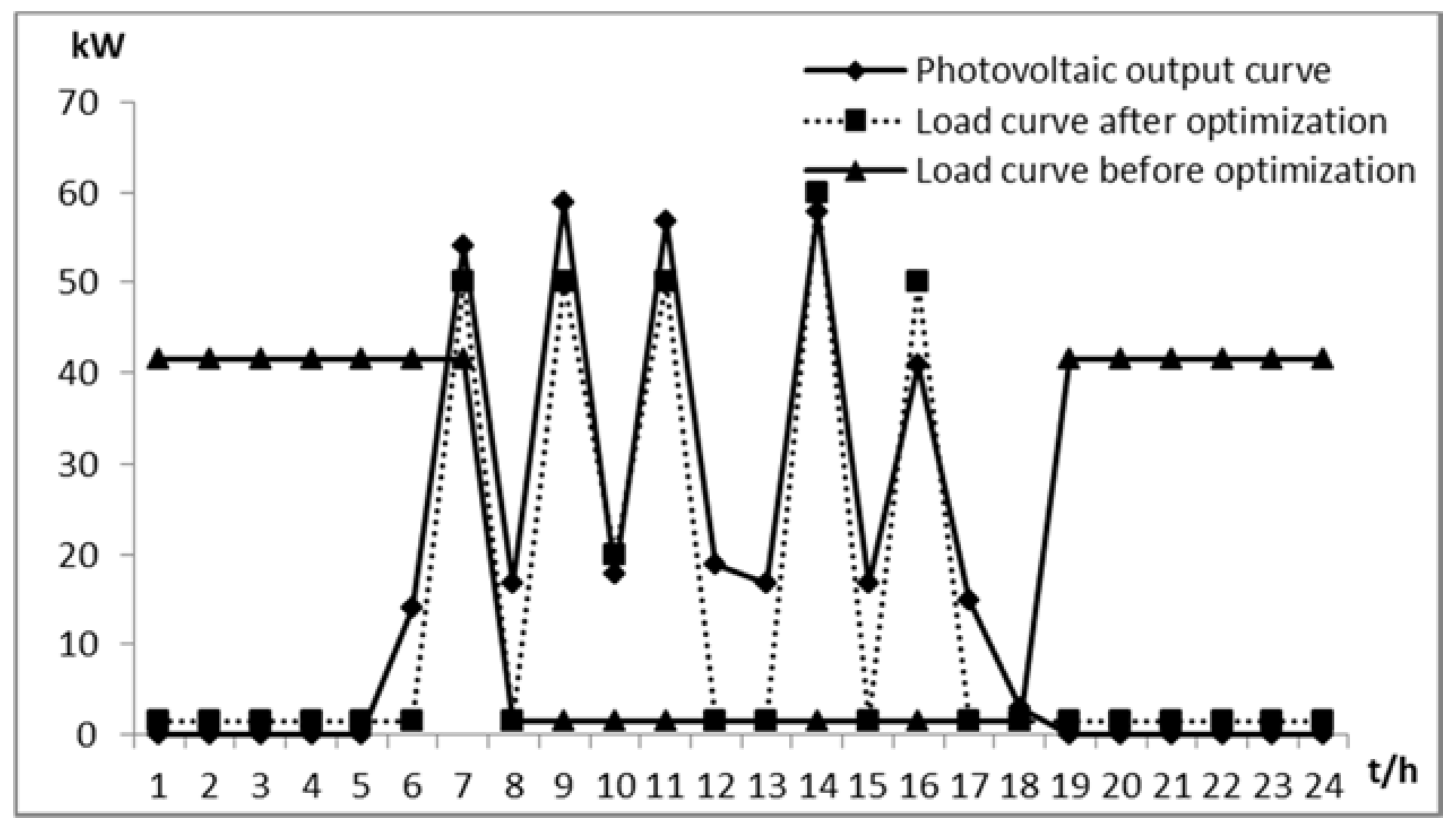
| Rainy day | 72.1 kWh | 18.6% | 277.1 kWh | 71.5% | 52.9% |
| Cloudy day after sunny day | 57.1 kWh | 8.9% | 551.8 kWh | 86.0% | 77.1% |
| Cloudy day after rainy day | 57.1 kWh | 8.9% | 582.4 kWh | 90.7% | 81.8% |
© 2018 by the authors. Licensee MDPI, Basel, Switzerland. This article is an open access article distributed under the terms and conditions of the Creative Commons Attribution (CC BY) license (http://creativecommons.org/licenses/by/4.0/).
Share and Cite
Wang, Y.; Niu, H.; Yang, L.; Wang, W.; Liu, F. An Optimization Method for Local Consumption of Photovoltaic Power in a Facility Agriculture Micro Energy Network. Energies 2018, 11, 1503. https://doi.org/10.3390/en11061503
Wang Y, Niu H, Yang L, Wang W, Liu F. An Optimization Method for Local Consumption of Photovoltaic Power in a Facility Agriculture Micro Energy Network. Energies. 2018; 11(6):1503. https://doi.org/10.3390/en11061503
Chicago/Turabian StyleWang, Yuzhu, Huanna Niu, Lu Yang, Weizhou Wang, and Fuchao Liu. 2018. "An Optimization Method for Local Consumption of Photovoltaic Power in a Facility Agriculture Micro Energy Network" Energies 11, no. 6: 1503. https://doi.org/10.3390/en11061503
APA StyleWang, Y., Niu, H., Yang, L., Wang, W., & Liu, F. (2018). An Optimization Method for Local Consumption of Photovoltaic Power in a Facility Agriculture Micro Energy Network. Energies, 11(6), 1503. https://doi.org/10.3390/en11061503